Model-based fault-detection and diagnosis ... - web page for staff
Model-based fault-detection and diagnosis ... - web page for staff
Model-based fault-detection and diagnosis ... - web page for staff

You also want an ePaper? Increase the reach of your titles
YUMPU automatically turns print PDFs into web optimized ePapers that Google loves.
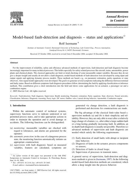
<strong>Model</strong>-<strong>based</strong> <strong>fault</strong>-<strong>detection</strong> <strong>and</strong> <strong>diagnosis</strong> – status <strong>and</strong> applications §<br />
Abstract<br />
Rolf Isermann *<br />
Institute of Automatic Control, Darmstadt University of Technology, Lab Control Eng., Process Automation,<br />
L<strong>and</strong>graf-Georg-Str 4, 64283 Darmstadt, Germany<br />
Received 25 October 2004; received in revised <strong>for</strong>m 8 December 2004; accepted 10 December 2004<br />
For the improvement of reliability, safety <strong>and</strong> efficiency advanced methods of supervision, <strong>fault</strong>-<strong>detection</strong> <strong>and</strong> <strong>fault</strong> <strong>diagnosis</strong> become<br />
increasingly important <strong>for</strong> many technical processes. This holds especially <strong>for</strong> safety related processes like aircraft, trains, automobiles, power<br />
plants <strong>and</strong> chemical plants. The classical approaches are limit or trend checking of some measurable output variables. Because they do not<br />
give a deeper insight <strong>and</strong> usually do not allow a <strong>fault</strong> <strong>diagnosis</strong>, model-<strong>based</strong> methods of <strong>fault</strong>-<strong>detection</strong> were developed by using input <strong>and</strong><br />
output signals <strong>and</strong> applying dynamic process models. These methods are <strong>based</strong>, e.g., on parameter estimation, parity equations or state<br />
observers. Also signal model approaches were developed. The goal is to generate several symptoms indicating the difference between nominal<br />
<strong>and</strong> <strong>fault</strong>y status. Based on different symptoms <strong>fault</strong> <strong>diagnosis</strong> procedures follow, determining the <strong>fault</strong> by applying classification or inference<br />
methods. This contribution gives a short introduction into the field <strong>and</strong> shows some applications <strong>for</strong> an actuator, a passenger car <strong>and</strong> a<br />
combustion engine.<br />
# 2005 Elsevier Ltd. All rights reserved.<br />
Keywords: Fault-<strong>detection</strong>; Fault <strong>diagnosis</strong>; Supervision; Health monitoring; Parameter estimation; Parity equations; State observers; Neural networks;<br />
Classification; Inference; Diagnostic reasoning; Fuzzy logic; DC motor; Outflow valve; Lateral driving behavior; Automobile; Combustion engine<br />
1. Introduction<br />
Annual Reviews in Control 29 (2005) 71–85<br />
Within the automatic control of technical systems,<br />
supervisory functions serve to indicate undesired or not<br />
permitted process states, <strong>and</strong> to take appropriate actions in<br />
order to maintain the operation <strong>and</strong> to avoid damage or<br />
accidents. The following functions can be distinguished:<br />
(a) monitoring: measurable variables are checked with<br />
regard to tolerances, <strong>and</strong> alarms are generated <strong>for</strong> the<br />
operator;<br />
(b) automatic protection: in the case of a dangerous process<br />
state, the monitoring function automatically initiates an<br />
appropriate counteraction;<br />
(c) supervision with <strong>fault</strong> <strong>diagnosis</strong>: <strong>based</strong> on measured<br />
variables, features are calculated, symptoms are<br />
§ An earlier version of this paper was presented at the 16th IFAC<br />
Symposium on Automatic Control in Aerospace, St. Petersburg, Russia,<br />
June 14–18, 2004.<br />
* Tel.: +49 6151 16 2114; fax: +49 6151 29 3445.<br />
E-mail address: risermann@iat.tu-darmstadt.de.<br />
1367-5788/$ – see front matter # 2005 Elsevier Ltd. All rights reserved.<br />
doi:10.1016/j.arcontrol.2004.12.002<br />
www.elsevier.com/locate/arcontrol<br />
generated via change <strong>detection</strong>, a <strong>fault</strong> <strong>diagnosis</strong> is<br />
per<strong>for</strong>med <strong>and</strong> decisions <strong>for</strong> counteractions are made.<br />
The big advantage of the classical limit-value <strong>based</strong> supervision<br />
methods (a) <strong>and</strong> (b) is their simplicity <strong>and</strong> reliability.<br />
However, they are only able to react after a relatively<br />
large change of a feature, i.e., after either a large sudden <strong>fault</strong><br />
or a long-lasting gradually increasing <strong>fault</strong>. In addition, an<br />
in-depth <strong>fault</strong> <strong>diagnosis</strong> is usually not possible. There<strong>for</strong>e (c)<br />
advanced methods of supervision <strong>and</strong> <strong>fault</strong> <strong>diagnosis</strong> are<br />
needed which satisfy the following requirements:<br />
(1) Early <strong>detection</strong> of small <strong>fault</strong>s with abrupt or incipient<br />
time behavior;<br />
(2) Diagnosis of <strong>fault</strong>s in the actuator, process components<br />
or sensors;<br />
(3) Detection of <strong>fault</strong>s in closed loops;<br />
(4) Supervision of processes in transient states.<br />
A general survey of supervision, <strong>fault</strong>-<strong>detection</strong> <strong>and</strong> <strong>diagnosis</strong><br />
methods is given in (Isermann, 1997). In the following<br />
model-<strong>based</strong> <strong>fault</strong>-<strong>detection</strong> methods are considered, which<br />
allow a deep insight into the process behavior.
72<br />
Fig. 1. General scheme of process model-<strong>based</strong> <strong>fault</strong>-<strong>detection</strong> <strong>and</strong> <strong>diagnosis</strong>.<br />
2. Process model-<strong>based</strong> <strong>fault</strong>-<strong>detection</strong> methods<br />
Different approaches <strong>for</strong> <strong>fault</strong>-<strong>detection</strong> using mathematical<br />
models have been developed in the last 20 years, see,<br />
e.g., (Chen & Patton, 1999; Frank, 1990; Gertler, 1998;<br />
Himmelblau, 1978; Isermann, 1984, 1997; Patton, Frank, &<br />
Clark, 2000; Willsky, 1976). The task consists of the<br />
<strong>detection</strong> of <strong>fault</strong>s in the processes, actuators <strong>and</strong> sensors by<br />
using the dependencies between different measurable<br />
signals. These dependencies are expressed by mathematical<br />
process models. Fig. 1 shows the basic structure of model<strong>based</strong><br />
<strong>fault</strong>-<strong>detection</strong>. Based on measured input signals U<br />
<strong>and</strong> output signals Y, the <strong>detection</strong> methods generate<br />
residuals r, parameter estimates ˆ Q or state estimates ˆx,<br />
which are called features. By comparison with the normal<br />
features (nominal values), changes of features are detected,<br />
leading to analytical symptoms s.<br />
For the application of model-<strong>based</strong> <strong>fault</strong>-<strong>detection</strong><br />
methods, the process configurations according to Fig. 2<br />
Fig. 2. Process configuration <strong>for</strong> model-<strong>based</strong> <strong>fault</strong>-<strong>detection</strong>: (a) SISO<br />
(single-input single-output); (b) SISO with intermediate measurements; (c)<br />
SIMO (single-input multi-output); (d) MIMO (multi-input multi-output).<br />
R. Isermann / Annual Reviews in Control 29 (2005) 71–85<br />
Fig. 3. Time-dependency of <strong>fault</strong>s: (a) abrupt; (b) incipient; (c) intermittent.<br />
have to be distinguished. With regard to the inherent<br />
dependencies used <strong>for</strong> <strong>fault</strong>-<strong>detection</strong>, <strong>and</strong> the possibilities<br />
<strong>for</strong> distinguishing between different <strong>fault</strong>s, the situation<br />
improves greatly from case (a) to (b) or (c) or (d), by the<br />
availability of some more measurements.<br />
2.1. Process models <strong>and</strong> <strong>fault</strong> modeling<br />
A <strong>fault</strong> is defined as an unpermitted deviation of at least<br />
one characteristic property of a variable from an<br />
acceptable behavior. There<strong>for</strong>e, the <strong>fault</strong> is a state that<br />
may lead to a malfunction or failure of the system. The<br />
time dependency of <strong>fault</strong>s can be distinguished, as shown<br />
in Fig. 3, abrupt <strong>fault</strong> (stepwise), incipient <strong>fault</strong> (driftlike),<br />
intermittent <strong>fault</strong>. With regard to the process models,<br />
the <strong>fault</strong>s can be further classified. According to Fig. 4<br />
additive <strong>fault</strong>s influence a variable Y by an addition of the<br />
<strong>fault</strong> f, <strong>and</strong>multiplicative <strong>fault</strong>s by the product of another<br />
variable U with f. Additive <strong>fault</strong>s appear, e.g., as offsets of<br />
sensors, whereas multiplicative <strong>fault</strong>s are parameter<br />
changes within a process.<br />
Now lumped-parameter processes are considered, which<br />
operate in open loop. The static behavior (steady states) is<br />
frequently expressed by a non-linear characteristic as shown<br />
in Table 1. Changes of parameters bi can be obtained by<br />
parameter estimation with, e.g., methods of least squares,<br />
<strong>based</strong> on measurements of different input–output pairs<br />
[Y j,U j]. This method is applicable, e.g., <strong>for</strong> valves, pumps,<br />
drives, engines.<br />
More in<strong>for</strong>mation on the process can usually be obtained<br />
with dynamic process models. Table 2 shows the basic<br />
input/output models in <strong>for</strong>m of a differential equation or a<br />
state space model as vector differential equation. Similar<br />
representations hold <strong>for</strong> non-linear processes <strong>and</strong> <strong>for</strong> multiinput<br />
multi-output processes, also in discrete-time.<br />
Fig. 4. Basic models of <strong>fault</strong>s: (a) additive <strong>fault</strong>; (b) multiplicative <strong>fault</strong>s.
Table 1<br />
Fault-<strong>detection</strong> of a non-linear static process via parameter estimation <strong>for</strong><br />
steady states<br />
2.2. Fault-<strong>detection</strong> with parameter estimation<br />
Process model-<strong>based</strong> methods require the knowledge of a<br />
usually dynamic process model in <strong>for</strong>m of a mathematical<br />
structure <strong>and</strong> parameters. For linear processes in continuous<br />
time the models can be impulse responses (weighting<br />
functions), differential equations of frequency responses.<br />
Corresponding models <strong>for</strong> discrete-time (after sampling) are<br />
impulse responses, difference equations or z-transfer<br />
functions. For <strong>fault</strong>-<strong>detection</strong> in general differential equa-<br />
Table 2<br />
Linear dynamic process models <strong>and</strong> <strong>fault</strong> modeling<br />
R. Isermann / Annual Reviews in Control 29 (2005) 71–85 73<br />
tions or difference equations are primarily suitable. In most<br />
practical cases the process parameters are partially not<br />
known or not known at all. Then, they can be determined<br />
with parameter estimation methods by measuring input <strong>and</strong><br />
output signals if the basic model structure is known. Table 3<br />
shows two approaches by minimization of the equation error<br />
<strong>and</strong> the output error. The first one is linear in the parameters<br />
<strong>and</strong> allows there<strong>for</strong>e direct estimation of the parameters<br />
(least squares estimates) in non-recursive or recursive <strong>for</strong>m.<br />
The second one needs numerical optimization methods <strong>and</strong><br />
there<strong>for</strong>e iterative procedures, but may be more precise<br />
under the influence of process disturbances. The symptoms<br />
are deviations of the process parameters DQ. As the process<br />
parameters Q ¼ f ðpÞ depend on physically defined process<br />
coefficients p (like stiffness, damping coefficients, resistance),<br />
determination of changes Dp allows usually a deeper<br />
insight <strong>and</strong> makes <strong>fault</strong> <strong>diagnosis</strong> easier (Isermann, 1992).<br />
Parameter estimation methods operate with adaptive process<br />
models, where only the model structure is known. They<br />
usually need a dynamic process input excitation <strong>and</strong> are<br />
especially suitable <strong>for</strong> the <strong>detection</strong> of multiplicative <strong>fault</strong>s.<br />
2.3. Fault-<strong>detection</strong> with observers<br />
If the process parameters are known, either state<br />
observers or output observers can be applied, Table 4. Fault<br />
modeling is then per<strong>for</strong>med with additive <strong>fault</strong>s fL at the
74<br />
Table 3<br />
Fault-<strong>detection</strong> with parameter estimation methods <strong>for</strong> dynamic processes<br />
input (additive actuator or process <strong>fault</strong>s) <strong>and</strong> fM at the<br />
output (sensor offset <strong>fault</strong>s).<br />
2.3.1. State observers<br />
The classical state observer can be applied if the <strong>fault</strong>s<br />
can be modeled as state variable changes Dx i as, e.g., <strong>for</strong><br />
leaks. In the case of multi-output processes special<br />
arrangements of observers were proposed:<br />
2.3.1.1. Dedicated observers <strong>for</strong> multi-output processes.<br />
Observer, excited by one output. One observer is driven<br />
by one sensor output. The other outputs y are reconstructed<br />
<strong>and</strong> compared with measured outputs y. This allows the<br />
<strong>detection</strong> of single sensor <strong>fault</strong>s (Clark, 1978).<br />
Bank of observers, excited by all outputs. Several state<br />
observers are designed <strong>for</strong> a definite <strong>fault</strong> signal <strong>and</strong> detected<br />
by a hypothesis test (Willsky, 1976).<br />
Bank of observers, excited by single outputs. Several<br />
observers <strong>for</strong> single sensor outputs are used. The estimated<br />
outputs y are compared with the measured outputs y. This<br />
allows the <strong>detection</strong> of multiple sensor <strong>fault</strong>s (Clark, 1978)<br />
(dedicated observer scheme).<br />
Bank of observers, excited by all outputs except one. As<br />
be<strong>for</strong>e, but each observer is excited by all outputs except one<br />
sensor output which is supervised (Frank, 1987).<br />
2.3.1.2. Fault-<strong>detection</strong> filters (<strong>fault</strong>-sensitive filters) <strong>for</strong><br />
multi-output processes. The feedback H of the state<br />
R. Isermann / Annual Reviews in Control 29 (2005) 71–85<br />
observer is chosen so that particular <strong>fault</strong> signals fL(t)<br />
change in a definite direction <strong>and</strong> <strong>fault</strong> signals fM(t) ina<br />
definite plane (Beard, 1971; Jones, 1973).<br />
2.3.2. Output observers<br />
Another possibility is the use of output observers (or<br />
unknown input observers) if the reconstruction of the state<br />
variables x(t) is not of interest. A linear trans<strong>for</strong>mation then<br />
leads to new state variables jðtÞ. The residuals r(t) can be<br />
designed such that they are independent of the unknown<br />
inputs v(t), <strong>and</strong> of the state by special determination of the<br />
matrices C j <strong>and</strong> T 2. The residuals then depend only on the<br />
additive <strong>fault</strong>s f L(t) <strong>and</strong> f M(t). However, all process model<br />
matrices must be known precisely. A comparison with the<br />
parity equation approach shows similarities.<br />
2.4. Fault-<strong>detection</strong> with parity equations<br />
A straight<strong>for</strong>ward model-<strong>based</strong> method of <strong>fault</strong>-<strong>detection</strong><br />
is to take a fixed model G M <strong>and</strong> run it parallel to the process,<br />
thereby <strong>for</strong>ming an output error, see Table 5.<br />
r 0 ðsÞ ¼½GpðsÞ GMðsÞŠuðsÞ (1)<br />
If Gp(s) =GM(s), the output error then becomes <strong>for</strong> additive<br />
input <strong>and</strong> output <strong>fault</strong>s, Table 2.<br />
r 0 ðsÞ ¼GpðsÞ fuðsÞþ fyðsÞ (2)
Table 4<br />
Fault-<strong>detection</strong> with observers <strong>for</strong> dynamic processes<br />
Another possibility is to generate an equation error (polynominal<br />
error) or an input error as in Table 6 (Gertler, 1998).<br />
The residuals depend in all cases only on the additive<br />
input <strong>fault</strong>s fu(t) <strong>and</strong> output <strong>fault</strong>s fy(t). The same procedure<br />
can be applied <strong>for</strong> multivariable processes by using a state<br />
space model, see Table 6.<br />
The derivatives of the signals can be obtained by state<br />
variable filters (Höfling, 1996). Corresponding equations<br />
exist <strong>for</strong> discrete-time <strong>and</strong> are easier to implement <strong>for</strong> the<br />
state space model. The residuals shown in Tables 5 <strong>and</strong> 6 left<br />
are direct residuals. If the parity equations are <strong>for</strong>mulated <strong>for</strong><br />
more than one input <strong>and</strong> one output, it becomes possible to<br />
generate structured residuals such that <strong>fault</strong>s do not<br />
influence all residuals. This improves the isolability of<br />
<strong>fault</strong>s (Gertler, 1998). For example, the components of<br />
matrix W <strong>for</strong> the state space model, Table 6 right, are<br />
selected such that, e.g., one measured variable has no impact<br />
on a specific residual. Parity equations are suitable <strong>for</strong> the<br />
R. Isermann / Annual Reviews in Control 29 (2005) 71–85 75<br />
<strong>detection</strong> <strong>and</strong> isolation of additive <strong>fault</strong>s. They are simpler to<br />
design <strong>and</strong> to implement than output observer-<strong>based</strong><br />
approaches <strong>and</strong> may be made to lead to the same results.<br />
2.5. Fault-<strong>detection</strong> with signal models<br />
Many measured signals y(t) show oscillations that are of<br />
either harmonic or stochastic nature, or both. If changes in<br />
these signals are related to <strong>fault</strong>s in the process, actuator or<br />
sensor, a signal analysis is a further source of in<strong>for</strong>mation.<br />
Especially <strong>for</strong> machine vibration, sensors <strong>for</strong> position, speed<br />
or acceleration are used to detect, <strong>for</strong> example, imbalance<br />
<strong>and</strong> bearing <strong>fault</strong>s (turbo machines), knocking (Diesel<br />
engines) or chattering (metal-grinding machines) (Kolerus,<br />
2000). But also signals from many other sensors, like<br />
electrical current, position, speed, <strong>for</strong>ce, flow <strong>and</strong> pressure,<br />
may show oscillations with a variety of higher frequencies<br />
than the usual process dynamic responses. The extraction of
76<br />
<strong>fault</strong>-relevant signal characteristics can in many cases be<br />
restricted to the amplitudes y0(v) or amplitude densities<br />
jy(iv)j within a certain b<strong>and</strong>width vmin v vmax of the<br />
signal by using of b<strong>and</strong>pass filters. Also parametric signal<br />
R. Isermann / Annual Reviews in Control 29 (2005) 71–85<br />
Table 5<br />
Fault-<strong>detection</strong> with different <strong>for</strong>ms of parity equations <strong>for</strong> linear input/output models<br />
Table 6<br />
Fault-<strong>detection</strong> with parity equations <strong>for</strong> dynamic processes<br />
models can be used, which allow the main frequencies <strong>and</strong><br />
their amplitudes to be directly estimated, <strong>and</strong> which are<br />
especially sensitive to small frequency changes. This is<br />
possible by modeling the signals as a superposition of<br />
damped sinusoids in the <strong>for</strong>m of discrete-time ARMA<br />
(autoregressive moving average) models (Burg, 1968;<br />
Neumann, 1991).<br />
3. Fault <strong>diagnosis</strong> methods<br />
The task of <strong>fault</strong> <strong>diagnosis</strong> consists of the determination<br />
of the type of <strong>fault</strong> with as many details as possible such as<br />
the <strong>fault</strong> size, location <strong>and</strong> time of <strong>detection</strong>. The diagnostic<br />
procedure is <strong>based</strong> on the observed analytical <strong>and</strong> heuristic<br />
symptoms <strong>and</strong> the heuristic knowledge of the process. The<br />
inputs to a knowledge-<strong>based</strong> <strong>fault</strong> <strong>diagnosis</strong> system are all<br />
available symptoms as facts <strong>and</strong> the <strong>fault</strong>-relevant knowledge<br />
about the process, mostly in heuristic <strong>for</strong>m. The<br />
symptoms may be presented just as binary values [0,1] or as,<br />
e.g., fuzzy sets to take gradual sizes into account.<br />
3.1. Classification methods<br />
If no further knowledge is available <strong>for</strong> the relations<br />
between features <strong>and</strong> <strong>fault</strong>s classification or pattern<br />
recognition methods can be used, Table 7. Here, reference<br />
vectors Sn are determined <strong>for</strong> the normal behavior. Then the<br />
corresponding input vectors S of the symptoms are
Table 7<br />
Methods of <strong>fault</strong> <strong>diagnosis</strong><br />
determined experimentally <strong>for</strong> certain <strong>fault</strong>s Fj. The<br />
relationship between F <strong>and</strong> S is there<strong>for</strong>e learned (or<br />
trained) experimentally <strong>and</strong> stored, <strong>for</strong>ming an explicit<br />
knowledge base. By comparison of the observed S with the<br />
normal reference S n, <strong>fault</strong>s F can be concluded.<br />
One distinguishes between statistical or geometrical<br />
classification methods, with or without certain probability<br />
functions (Tou & Gonzalez, 1974). A further possibility is<br />
the use of neural networks because of their ability to<br />
approximate non-linear relations <strong>and</strong> to determine flexible<br />
decision regions <strong>for</strong> F in continuous or discrete <strong>for</strong>m<br />
(Leonhardt, 1996). By fuzzy clustering the use of fuzzy<br />
separation areas is possible.<br />
3.2. Inference methods<br />
For some technical processes, the basic relationships<br />
between <strong>fault</strong>s <strong>and</strong> symptoms are at least partially known.<br />
Then this a priori knowledge can be represented in causal<br />
relations: <strong>fault</strong> ! events ! symptoms. Table 7 shows a<br />
simple causal network, with the nodes as states <strong>and</strong> edges as<br />
relations. The establishment of these causalities follows the<br />
<strong>fault</strong>-tree analysis (FTA), proceeding from <strong>fault</strong>s through<br />
intermediate events to symptoms (the physical causalities)<br />
or the event-tree analysis (ETA), proceeding from the<br />
symptoms to the <strong>fault</strong>s (the diagnostic <strong>for</strong>ward-chaining<br />
causalities). To per<strong>for</strong>m a <strong>diagnosis</strong>, this qualitative<br />
R. Isermann / Annual Reviews in Control 29 (2005) 71–85 77<br />
knowledge can now be expressed in <strong>for</strong>m of rules: IF<br />
THEN . The condition part<br />
(premise) contains facts in the <strong>for</strong>m of symptoms Si as<br />
inputs, <strong>and</strong> the conclusion part includes events Ek <strong>and</strong> <strong>fault</strong>s<br />
Fj as a logical cause of the facts. If several symptoms<br />
indicate an event or <strong>fault</strong>, the facts are associated by AND<br />
<strong>and</strong> OR connectives, leading to rules in the <strong>for</strong>m<br />
IF < S 1 AND S 2 > THEN <br />
IF < E 1 OR E 2 > THEN .<br />
For the establishment of this heuristic knowledge several<br />
approaches exist, see (Torasso & Console, 1974). In the<br />
classical <strong>fault</strong>-tree analysis the symptoms <strong>and</strong> events are<br />
considered as binary variables, <strong>and</strong> the condition part of the<br />
rules can be calculated by Boolean equations <strong>for</strong> parallelserial-connection,<br />
see, e.g. (Barlow & Proschan, 1975; Freyermuth,<br />
1993). However, this procedure has not proved to<br />
be successful because of the continuous nature of <strong>fault</strong>s <strong>and</strong><br />
symptoms. For the <strong>diagnosis</strong> of technical processes approximate<br />
reasoning is more appropriate. A recent survey on<br />
learning methods <strong>for</strong> rule-<strong>based</strong> <strong>diagnosis</strong> is given in (Füssel<br />
& Isermann, 2000).<br />
The summary of some basic <strong>fault</strong>-<strong>detection</strong> <strong>and</strong> <strong>diagnosis</strong><br />
methods presented in Sections 2 <strong>and</strong> 3 was limited to linear<br />
processes mainly. Some of the methods can also be directly<br />
applied <strong>for</strong> non-linear processes, as e.g., signal analysis,<br />
parity equations <strong>and</strong> parameter estimation. However, all the<br />
methods have to be adapted to the real processes. In this<br />
sense the basic methods should be considered as ‘‘tools’’,<br />
which have to be combined properly in order to meet the<br />
practical requirements <strong>for</strong> real <strong>fault</strong>s of real processes.<br />
4. Applications of model- <strong>and</strong> signal-<strong>based</strong> <strong>fault</strong><br />
<strong>diagnosis</strong><br />
In the following some results from case studies <strong>and</strong> indepth<br />
investigations of model-<strong>based</strong> <strong>fault</strong>-<strong>detection</strong> methods<br />
are briefly described. The examples are selected such that<br />
they show different approaches <strong>and</strong> process adapted<br />
solutions which can be transferred to other similar technical<br />
processes.<br />
4.1. Fault <strong>diagnosis</strong> of a cabin pressure outflow valve<br />
actuator of a passenger aircraft<br />
The air pressure control in passenger aircraft is manipulated<br />
by DC motor driven outflow valves. The design of the<br />
outflow valve is made <strong>fault</strong> tolerant by two brushless DC<br />
motors which operate over the gear to a lever mechanism<br />
moving the flap, Fig. 5. The two DC motors <strong>for</strong>m a<br />
duplex system with dynamic redundancy <strong>and</strong> cold st<strong>and</strong>by,<br />
Fig. 6. There<strong>for</strong>e, a <strong>fault</strong>-<strong>detection</strong> <strong>for</strong> both DC motors is<br />
required to switch from the possibly <strong>fault</strong>y one to the<br />
st<strong>and</strong>by motor.
78<br />
Fig. 5. Actuator servo-drive <strong>for</strong> cabin pressure control (Nord Micro).<br />
In the following it is shown how the <strong>fault</strong>-<strong>detection</strong> was<br />
realized by combining parameter estimation <strong>and</strong> parity<br />
equations with implementation on a low cost microcontroller<br />
(Moseler & Isermann, 2000a; Moseler, Heller, &<br />
Isermann, 1999; Moseler & Müller, 2000).<br />
A detailed model of the brushless DC motor <strong>for</strong> all three<br />
phases is given in (Isermann, 2003a; Moseler et al., 1999). It<br />
could be shown that <strong>for</strong> the case of <strong>fault</strong>-<strong>detection</strong> averaged<br />
values (by low pass filter) of the voltage U(t) <strong>and</strong> the current<br />
I(t) to the stator coils can be assumed. This leads to the<br />
voltage equation of the electrical subsystem.<br />
UðtÞ kEvrðtÞ ¼RIðtÞ (3)<br />
with R the overall resistance <strong>and</strong> k E the magnetic flux<br />
linkage. The generated rotor torque is proportional to the<br />
effective magnetic flux linkage k T < k E<br />
TrðtÞ kTIðtÞ (4)<br />
(In ideal cases kE = kT). The mechanical part is then<br />
described by<br />
Jr ˙vrðtÞ ¼kTIðtÞ TfðtÞ TLðtÞ (5)<br />
R. Isermann / Annual Reviews in Control 29 (2005) 71–85<br />
with the moment of inertia J r, <strong>and</strong> the Coulomb friction<br />
torque<br />
TfðtÞ ¼cf sign vrðtÞ (6)<br />
<strong>and</strong> the load torque TL(t). The gear ratio v relates the motor<br />
shaft position fr to the flap position fg<br />
’ g ¼ ’ r<br />
(7)<br />
n<br />
with n = 2500. The load torque of the flap is a non-linear<br />
function of the position fg<br />
TL ¼ cs f ð’ gÞ<br />
<strong>and</strong> is approximately known around the steady-state operation<br />
point. (For the experiments the flap was replaced by a<br />
lever with a spring). For <strong>fault</strong>-<strong>detection</strong> following measurements<br />
are available: U(t), I(t), fr(t), fg(t). Using the notation<br />
yðtÞ ¼c T ðtÞu (8)<br />
two equations were used <strong>for</strong> parameter estimation<br />
electrical subsystem<br />
yðtÞ ¼UðtÞ; c T ðtÞ ¼½IðtÞvrðtÞŠ;<br />
u T ¼½RkEŠ<br />
mechanical subsystem<br />
yðtÞ ¼kTIðtÞ cs f ð’ gðtÞ Jr ˙vrðtÞÞ<br />
c T ðtÞ ¼½sign vrtŠ; u T ¼½cfŠðJr knownÞ<br />
(9)<br />
(10)<br />
Hence, three parameters R _ , k _<br />
E, <strong>and</strong> c _<br />
f are estimated. Various<br />
parameter estimation methods were applied like: recursive<br />
least squares (RLS), discrete square root filtering (DSFI),<br />
fast DSFI (FSDFI), normalized least mean squares (NLMS)<br />
<strong>and</strong> compared. The parity equations are obtained from the<br />
basic two Eqs. (3) <strong>and</strong> (5) by assuming known parameters<br />
(obtained from parameter estimation)<br />
r1ðtÞ ¼UðtÞ RIðtÞ kEvrðtÞ (11)<br />
r2ðtÞ ¼kTIðtÞ Jr ˙vrðtÞ cf sign vrðtÞ cs f ð’ gÞ (12)<br />
r3ðtÞ ¼UðtÞ<br />
Fig. 6. Redundant DC motor drive system <strong>for</strong> the outflow valve.<br />
R<br />
ðJr ˙vrðtÞþcs f ð’ gÞþcf sign vrðtÞ<br />
kT<br />
þ kEvrðtÞ (13)
4ðtÞ ¼’ gðtÞ<br />
’ rðtÞ<br />
v<br />
(14)<br />
Each of the residuals is decoupled from one measured<br />
signal. r1 is independent from fg, r2 from U, r3 from I, r4<br />
from all but fr.(fr is assumed to be correct. It can directly be<br />
supervised by a logic evaluation within the motor electronics).<br />
Fig. 7 shows measured signals, parameter estimates<br />
<strong>and</strong> residuals <strong>for</strong> five different implemented <strong>fault</strong>s. The<br />
actuator was operating in closed loop with slow triangle<br />
changes of the reference variable (setpoint). The <strong>fault</strong><strong>detection</strong><br />
methods, including differentiating filter (SVF)<br />
were implemented on a digital signal processor TI TMS<br />
320 C40 with signal sampling period T0 = 1 ms. The results<br />
<strong>for</strong> <strong>fault</strong>-<strong>detection</strong> are summarized in Table 8.<br />
The sign <strong>and</strong> size of changes <strong>for</strong> the parameter estimates<br />
with FDSFI clearly allow to identify the parametric <strong>fault</strong>s<br />
<strong>and</strong> <strong>for</strong> the parity residuals the respective additive (offset)<br />
sensor <strong>fault</strong>s. But there are also cross couplings: <strong>for</strong> parametric<br />
<strong>fault</strong>s some residuals show changes <strong>and</strong> <strong>for</strong> sensor<br />
additive <strong>fault</strong>s some parameter estimates change (except <strong>for</strong><br />
fg), which can all be interpreted by the equations used.<br />
According to (Gertler, 1998) the symptom pattern is weakly<br />
isolating as a parametric <strong>fault</strong> of R <strong>and</strong> an additive <strong>fault</strong> in U<br />
differ only in one symptom. However, all <strong>fault</strong>s can be<br />
isolated. Including the st<strong>and</strong>ard deviation of the symptoms<br />
isolability can be improved (Moseler, 2001). By processing<br />
eight symptoms with a rule-<strong>based</strong> fuzzy-logic <strong>diagnosis</strong><br />
system, finally 10 different <strong>fault</strong>s could be diagnosed (Moseler<br />
<strong>and</strong> Müller, 2000b; Moseler, 2001).<br />
If the input signal U stays approximately constant, only<br />
parity equations should be applied, which then may indicate<br />
<strong>fault</strong>s. Then <strong>for</strong> isolating or diagnosing the <strong>fault</strong>s a test<br />
signal on U can be applied <strong>for</strong> short time to gain deeper<br />
in<strong>for</strong>mation. Hence, by applying both parameter estimation<br />
<strong>and</strong> parity equations a good <strong>fault</strong> coverage can be obtained.<br />
Because the position sensors of the rotor fr <strong>and</strong> the shaft fg<br />
yield redundant in<strong>for</strong>mation, sensor <strong>fault</strong>-<strong>detection</strong> <strong>for</strong> fg<br />
was used to reconfigure the closed loop after failure of fg<br />
by using fr as control variable (Moseler, 2001). The<br />
described combined <strong>fault</strong>-<strong>detection</strong> methodology needs<br />
about 8 ms calculation time on a 16 bit microcontroller.<br />
There<strong>for</strong>e, online implementation in a smart actuator is<br />
possible by only measuring four easy accessible variables<br />
U, I <strong>and</strong> vr <strong>and</strong> fg.<br />
4.2. Supervision of the lateral driving behavior of<br />
passenger cars<br />
Based on theoretical modeling of the lateral behavior of a<br />
passenger car, the characteristic velocity is considered as a<br />
parameter determining the kind of the steering behavior, like<br />
understeering or oversteering. This characteristic value is<br />
used as a ‘‘<strong>fault</strong>-<strong>detection</strong> feature’’ due to Fig. 1 to classify the<br />
behavior with regard to normal or critical driving behavior <strong>and</strong><br />
such indicating also <strong>fault</strong>y behavior, like instability.<br />
R. Isermann / Annual Reviews in Control 29 (2005) 71–85 79<br />
Fig. 7. Resulting symptoms from parameter estimation <strong>and</strong> parity equations<br />
by measuring U(t), I(t), v(t),f g(t) <strong>and</strong> f r(t).<br />
Table 8<br />
Parameter deviations <strong>and</strong> parity equation residuals <strong>for</strong> different actuator<br />
<strong>fault</strong>s (0 no significant change; + increase; ++ large increase;<br />
large decrease)<br />
decrease;<br />
Faults Parameter estimates Residuals of parity equations<br />
ˆR ˆ kE ĉf r1 r2 r3 r4<br />
Incr. R + 0 0 + 0 + 0<br />
Incr. c f 0 0 ++ + ++ 0<br />
Offset U + + 0 ++ 0 ++ 0<br />
Offset fg 0 0 0 + 0 0 0<br />
Offset Ib ++ ++ ++ 0
80<br />
Fig. 8. Scheme <strong>for</strong> modeling the lateral vehicle behavior with a one-track<br />
model.<br />
4.2.1. Vehicle model<br />
For deriving the lateral dynamics, a coordinate system is<br />
fixed to the center of gravity (CG) <strong>and</strong> Newton’s lawsare<br />
applied, Fig. 8. Roll, pitch, bounce, <strong>and</strong> deceleration dynamics<br />
are neglected to reduce the model to two degrees of freedom:<br />
the lateral position <strong>and</strong> yaw angle states. The resulting nonlinear<br />
dynamic model, known as the one-track model, is<br />
2<br />
¨y<br />
¨c ¼<br />
6<br />
4<br />
c 0<br />
aF þ caR þ m˙v<br />
mv<br />
6<br />
þ 6<br />
4<br />
caRlR c 0<br />
aF lF<br />
2<br />
Jzv<br />
3<br />
7<br />
c 0<br />
aF<br />
mist<br />
c 0<br />
aFlF 5 dst<br />
Jsist<br />
caRlR c 0<br />
aF lF<br />
caRl 2 R<br />
mv<br />
þ c0<br />
Jzv<br />
aF l2 F<br />
3<br />
7<br />
5<br />
˙y<br />
˙c<br />
(15)<br />
see, e.g. (Isermann, 2001). The symbols are explained in<br />
Table 9. Although the one-track model is relatively simple, it<br />
has been proven to be a good approximation <strong>for</strong> vehicle<br />
dynamics when lateral acceleration is limited to 0.4 g on<br />
normal dry asphalt roads.<br />
4.2.2. Stability of vehicles<br />
Based on the state equation of the one-track model the<br />
characteristic equation det (s I -A) = 0 of the lateral vehicle<br />
dynamics becomes<br />
a1<br />
zfflfflfflfflfflfflfflfflfflfflfflfflfflfflfflfflfflfflfflfflfflfflfflfflfflffl}|fflfflfflfflfflfflfflfflfflfflfflfflfflfflfflfflfflfflfflfflfflfflfflfflfflffl{<br />
s 2 þ ðJz þ ml2 FÞc0aF þðJz þ ml2 RÞcaR s<br />
Jzmv<br />
þ c0aF<br />
caRðlF þ lRÞ 2 þ mv2ðcaRlR c 0<br />
aFlFÞ Jzmv2 a0<br />
zfflfflfflfflfflfflfflfflfflfflfflfflfflfflfflfflfflfflfflfflfflfflfflfflfflfflfflfflfflfflfflfflffl}|fflfflfflfflfflfflfflfflfflfflfflfflfflfflfflfflfflfflfflfflfflfflfflfflfflfflfflfflfflfflfflfflffl{<br />
¼ 0 (16)<br />
According to the Hurwitz stability criterion, stability<br />
requires that a1 > 0 <strong>and</strong> a0 > 0. As a1 > 0 is always satis-<br />
R. Isermann / Annual Reviews in Control 29 (2005) 71–85<br />
Table 9<br />
Symbols <strong>for</strong> vehicle variables <strong>and</strong> parameters<br />
Symbol Description Value Unit<br />
x Longitudinal position error – [m]<br />
y Lateral position error – [m]<br />
z Vertical position error – [m]<br />
c Yaw angle – [rad]<br />
d Steering angle – [rad]<br />
dst Steering wheel angle – [rad]<br />
b Side slip angle – [rad]<br />
m vehicle mass 1720 [kg]<br />
Jz Mom. of inertia, z-axis 2275 [kg m 2 ]<br />
v Longitudinal velocity – [m/s]<br />
c’aF Effective front wheel cornering stiffness 50000 [N/rad]<br />
caR Rear wheel cornering stiffness 60000 [N/rad]<br />
lF,lR Length of front, rear axle from CG 1.3/1.43 [m]<br />
l Length between front <strong>and</strong> rear axle 2.73 [m]<br />
ist Steering system gear ratio 13.5 [–]<br />
r Radius – [m]<br />
Fxr Longitudinal <strong>for</strong>ce acting on rear tire – [N]<br />
FxF Longitudinal <strong>for</strong>ce acting on front tire – [N]<br />
FyR Side <strong>for</strong>ce acting on rear tire – [N]<br />
FyF Side <strong>for</strong>ce acting on front tire – [N]<br />
fied, because no negative values arise, only a0 has to be<br />
considered. With the characteristic velocity<br />
v 2 c<br />
chðtÞ ¼<br />
0<br />
2<br />
aFðtÞcaRðtÞ mðcaRðtÞlR c 0<br />
aFðtÞlFÞ (17)<br />
the following stability condition results:<br />
a0<br />
zfflfflfflfflfflfflfflfflfflfflfflfflfflfflfflfflfflfflfflfflfflfflfflfflfflfflfflfflfflfflfflffl}|fflfflfflfflfflfflfflfflfflfflfflfflfflfflfflfflfflfflfflfflfflfflfflfflfflfflfflfflfflfflfflffl{<br />
c 0<br />
aF caRðlF þ lRÞ 2 þ mv 2 ðcaRlR c 0<br />
aF lF<br />
> 0 ) 1 þ v2<br />
v2 > 0<br />
ch<br />
(18)<br />
4.2.3. Circular test drive<br />
A stationary circular test drive is now assumed. The<br />
dynamic equation of motion leads to the algebraic<br />
relationship<br />
˙cðtÞ 1 vðtÞ<br />
¼<br />
dstðtÞ istl 1 þðvðtÞ=vchðtÞÞ 2<br />
(19)<br />
With the measured steering wheel angle dst as the input, the<br />
velocity vðtÞ <strong>and</strong> the yaw rate ˙cðtÞ as the output, the<br />
quadratic characteristic velocity v2 chðtÞ follows from (19)<br />
v 2 chðtÞ ¼<br />
v 2 ðtÞ<br />
1 ðdstðtÞvðtÞ= ˙cðtÞistlÞ<br />
(20)<br />
Introducing the steering wheel angle dst,0(t) <strong>for</strong> neutral<br />
steering yields in (19) with n nch<br />
dst<br />
dst;0<br />
¼ 1 þ v2<br />
v 2 ch<br />
(21)<br />
This leads to the definition of neutral-, under- <strong>and</strong> oversteering:
Fig. 9. Steering gain ratio in dependence on the speed n 2 <strong>and</strong> characteristic<br />
velocity v 2 ch .<br />
if v2 ch ! 1then neutralsteering behavior;<br />
if v2 ch > 0 then understeering behavior;<br />
if v2 ch ¼ 0 then indifferent behavior;<br />
if v2 ch < 0 then oversteering behavior.<br />
Fig. 9 shows the different situations.<br />
4.2.4. Characteristic velocity stability indicator CVSI<br />
A driving situation <strong>detection</strong> is developed via the<br />
calculation of the characteristic velocity nch <strong>and</strong> a driving<br />
situation decision logic. The input of the model is the<br />
steering wheel angle signal dst. As output signal the yaw rate<br />
sensor ˙c can be used to calculate the characteristic velocity<br />
n ch, see (20). With help of the on-line calculated<br />
characteristic velocity n ch, the over ground velocity v, <strong>and</strong><br />
the steering wheel angle d st the current driving situation can<br />
be detected. For small steering angles dst < dst,L, it is<br />
Table 10<br />
Classification of different driving conditions (L: logical AND)<br />
R. Isermann / Annual Reviews in Control 29 (2005) 71–85 81<br />
assumed that the driving condition is mainly a straight run,<br />
just compensating <strong>for</strong> disturbances. If dst dst,L cornering<br />
can be assumed. Then a classification of different driving<br />
situations can be made as shown in Table 10 (Börner,<br />
Andréani, Albertos, & Isermann, 2002) with an indicator<br />
called characteristic velocity stability indicator (CVSI).<br />
4.2.5. Experimental results<br />
The following results are <strong>based</strong> on experimental data,<br />
which have been obtained using an Opel Omega vehicle on<br />
an airfield runway (Börner, 2004).<br />
The test vehicle is equipped with special sensors <strong>for</strong><br />
measuring the following signals: the steering wheel angle<br />
dst, lateral acceleration ¨y, yaw rate ˙c, <strong>and</strong> ABS velocity n1.4.<br />
The passenger cars velocity v has a large influence on the<br />
vehicles stability. Fig. 10 shows the behavior <strong>for</strong> a double<br />
lane change. After starting cornering, the vehicle shows first<br />
understeering, then neutral steering <strong>and</strong> oversteering<br />
behavior. At t = 16.4 <strong>and</strong> 17.8 s <strong>for</strong> a short time unstable<br />
behavior with counter steering can be observed. Further<br />
examples are shown in (Börner, 2004).<br />
4.3. Combustion engines<br />
Because of increased sensors, actuators <strong>and</strong> electronic<br />
functions the <strong>diagnosis</strong> of <strong>fault</strong>s in combustion engines gets<br />
more complicated. However, model-<strong>based</strong> <strong>fault</strong>-<strong>detection</strong><br />
offers new approaches by using the electronic control units<br />
not only <strong>for</strong> control but also <strong>for</strong> increased model-<strong>based</strong> <strong>fault</strong><br />
<strong>diagnosis</strong>. There<strong>for</strong>e an overall <strong>fault</strong>-<strong>diagnosis</strong> system <strong>for</strong><br />
Diesel engines is briefly described. The inlet system, the<br />
injection <strong>and</strong> combustion as well as the exhaust system have<br />
been considered. The methods are <strong>based</strong> on an appropriate<br />
signal processing of measurable signals using signal- <strong>and</strong><br />
process models to generate physically related features,
82<br />
residuals <strong>and</strong> symptoms. Former publications on <strong>fault</strong><strong>detection</strong><br />
of gasoline engines are, <strong>for</strong> example (Krishnaswami,<br />
Luth, & Rizzoni, 1995; Rizzoni & Samimy, 1996) or<br />
(Nielsen & Nyberg, 1993).<br />
Fig. 11 shows the concept <strong>for</strong> the developed model-<strong>based</strong><br />
<strong>fault</strong>-<strong>detection</strong> <strong>and</strong> <strong>diagnosis</strong> of the complete engine, see<br />
also (Kimmich, Schwarte, & Isermann, 2005; Schwarte,<br />
Kimmich, & Isermann, 2002). The engine is partitioned in<br />
three major subsystems: intake system, injection, combustion<br />
<strong>and</strong> crankshaft system as well the exhaust gas system.<br />
R. Isermann / Annual Reviews in Control 29 (2005) 71–85<br />
Fig. 10. Double lane change with speed v = 12 m/s: (a) steering angle; (b) yaw-rate; (c) CVSI: characteristic velocity indicator.<br />
The actuators are comm<strong>and</strong>ed by the electronic control unit<br />
<strong>and</strong> act on different components of the combustion engine.<br />
In addition to the available mass production sensors only<br />
very few additional sensors are used. For each major<br />
subsystem, <strong>fault</strong>-<strong>detection</strong> methods are developed to detect<br />
<strong>fault</strong>s in the shown components <strong>and</strong> to generate symptoms.<br />
Then the symptoms are processed with <strong>diagnosis</strong> methods to<br />
decide on <strong>fault</strong>s according to their type <strong>and</strong> location. The<br />
investigated engine is an Opel 2 liter, 4 cylinder, 16 valve<br />
turbo charge DI Diesel engine with a power of 74 kW <strong>and</strong> a<br />
Fig. 11. Concept of a modular model-<strong>based</strong> <strong>fault</strong>-<strong>detection</strong> system of the complete combustion engine. Module 1: intake system; module 2: injection,<br />
combustion; module 3: exhaust system.
Fig. 12. Air path of the intake system with sensors <strong>and</strong> considered <strong>fault</strong>s.<br />
torque of 205 Nm. The engine employs exhaust gas<br />
recirculation <strong>and</strong> a variable swirl of the inlet gas <strong>for</strong><br />
emission reduction.<br />
Only the intake system can be considered here as<br />
example. As shown in Fig. 12 the air flows through the air<br />
filter, air mass flow sensor, compressor, intercooler <strong>and</strong> inlet<br />
manifold.<br />
Measured input variables are the engine speed, the pulse<br />
width modulated signals <strong>for</strong> the EGR <strong>and</strong> SFA (swirl flaps)<br />
R. Isermann / Annual Reviews in Control 29 (2005) 71–85 83<br />
Fig. 13. Fault <strong>diagnosis</strong> structure of the intake system.<br />
as well as the atmospheric pressure <strong>and</strong> temperature, see<br />
Fig. 13.<br />
Measured output variables are manifold pressure, the<br />
manifold temperature <strong>and</strong> the air mass flow. The engine<br />
pumping, describing the air mass flow into the engine, was<br />
modeled with a semi-physical neural network model<br />
(LOLIMOT). It is a mean value model of one working<br />
cycle neglecting the periodic working principle. For the <strong>fault</strong><br />
free description of the intake system 5 static reference<br />
Fig. 14. Residual deflection in dependency on <strong>fault</strong>s (online); 2000 min 1 , 130 Nm, p 2,i = 1.5 bar, air flow 165 kg/h.
84<br />
models were identified, which describe the volumetric<br />
efficiency, the amplitude of air mass flow oscillation, the<br />
phase of air mass flow oscillation, the amplitude of boost<br />
pressure oscillation depending on engine speed <strong>and</strong><br />
manifold pressure. The reference models were identified<br />
<strong>for</strong> a closed EGR valve <strong>and</strong> opened swirl flaps actuator with<br />
a quasi stationary identification cycle. The identified nonlinear<br />
reference models calculating special features are used<br />
to set up five independent parity equations yielding five<br />
residuals. The results of real-time <strong>fault</strong>-<strong>detection</strong> are<br />
presented in Fig. 14 <strong>for</strong> an exemplary operating point.<br />
Several <strong>fault</strong>s were temporarily built into the intake system.<br />
The <strong>fault</strong>-<strong>detection</strong> thresholds are marked by dotted lines.<br />
The reference models <strong>for</strong> the volumetric efficiency,<br />
amplitude air mass flow oscillation, amplitude boost<br />
pressure oscillation, show the expected behavior in order<br />
to isolate the different <strong>fault</strong>s. Similar methods were<br />
developed <strong>for</strong> the other parts of the Diesel engine,<br />
(Isermann, Schwarte, & Kimmich, 2004).<br />
5. Conclusion<br />
After a short introduction into model-<strong>based</strong> <strong>fault</strong><strong>detection</strong><br />
methods, like parameter estimation, observers<br />
<strong>and</strong> parity equations, <strong>and</strong> <strong>fault</strong>-<strong>diagnosis</strong> methods, like<br />
classification <strong>and</strong> inference methods, three application<br />
examples were shown. For a DC motor actuator of an<br />
aircraft cabin pressure control the combination of parameter<br />
estimation <strong>and</strong> parity equations allows the <strong>detection</strong> of<br />
several parametric <strong>and</strong> additive <strong>fault</strong>s by using four<br />
measurements, followed by the <strong>fault</strong> <strong>diagnosis</strong> with<br />
fuzzy-logic inferencing. Based on a dynamic one-track<br />
model of a passenger car a time-varying parameter, the<br />
characteristic velocity, can be calculated by measurement of<br />
three drive dynamic variables. A classification scheme then<br />
indicates different lateral driving conditions, from stable<br />
understeering to unstable countersteering. For <strong>fault</strong> <strong>diagnosis</strong><br />
of Diesel engines three <strong>detection</strong> modules are<br />
proposed to generate symptoms <strong>based</strong> on mainly production-type<br />
sensors. The symptoms are generated with nonlinear<br />
output error <strong>and</strong> input error parity equations <strong>for</strong><br />
special model-<strong>based</strong> characteristic quantities like volumetric<br />
efficiency, oscillations of pressure, flow <strong>and</strong> (not shown<br />
here) <strong>for</strong> angular speed <strong>and</strong> oxygen content. The generation<br />
of about 20 symptoms then allow an in-depth <strong>fault</strong> <strong>diagnosis</strong>,<br />
e.g., by a fuzzy logic inference scheme.<br />
The shown examples are only a small sample of many<br />
other developed <strong>and</strong> experimentally tested <strong>fault</strong>-<strong>detection</strong><br />
<strong>and</strong> <strong>fault</strong>-<strong>diagnosis</strong> procedures, like <strong>for</strong> pneumatic <strong>and</strong><br />
hydraulic actuators, robots <strong>and</strong> machine tools, AC motors<br />
with centrifugal <strong>and</strong> oscillating pumps, SI engines <strong>and</strong><br />
automotive brake <strong>and</strong> active suspension systems. In all<br />
cases the model-<strong>based</strong> <strong>fault</strong>-<strong>detection</strong> <strong>and</strong> <strong>diagnosis</strong> has<br />
demonstrated a big step <strong>for</strong>ward compared to limit <strong>and</strong><br />
trend checking of some directly measurable variables.<br />
R. Isermann / Annual Reviews in Control 29 (2005) 71–85<br />
However, the methods have to be adapted to the physical<br />
properties of the processes <strong>and</strong> their sensor signals <strong>and</strong><br />
some ef<strong>for</strong>t is needed to obtain the mostly non-linear<br />
dynamic models. In many cases the combination of<br />
parameter estimation <strong>and</strong> parity equations, the last one <strong>for</strong><br />
directly measured <strong>and</strong> calculated characteristic quantities,<br />
has proven to result in a good <strong>fault</strong> <strong>diagnosis</strong> coverage <strong>and</strong><br />
to be most efficient.<br />
References<br />
Barlow, R. E., & Proschan, F. (1975). Statistical theory of reliability <strong>and</strong> life<br />
testing. Holt: Rinehart & Winston Inc.<br />
Beard, R. V. (1971). Failure accommodation in linear systems through selfreorganization.<br />
Rept. MVT-71-1. Cambridge, MA: Man Vehicle<br />
Laboratory.<br />
Börner, M. (2004). Adaptive Querdynamikmodelle für Personenkraftfahrzeuge<br />
- Fahrzust<strong>and</strong>serkennung und Sensorfehlertoleranz. Fortschr.-<br />
Ber. VDI Reihe 12 No. 563. Düsseldorf: VDI Verlag.<br />
Börner M., Andréani, L., Albertos, P., & Isermann, R. (2002). Detection of<br />
Lateral Vehicle Driving Conditions Based on the Characteristic Velocity.<br />
In IFAC World Congress 2002. Barcelona, Spain.<br />
Burg, J. P. (1968). A new analysis technique <strong>for</strong> time series data. In NATO<br />
Advanced Study Institute on Signal Processing with Emphasis on<br />
Underwater Acoustics.<br />
Chen, J., & Patton, R. J. (1999). Robust model-<strong>based</strong> <strong>fault</strong> <strong>diagnosis</strong> <strong>for</strong><br />
dynamic systems. Boston: Kluwer.<br />
Clark, R. N. (1978). A simplified instrument <strong>detection</strong> scheme. IEEE<br />
Transactions on Aerospace <strong>and</strong> Electronic Systems, 14(456–465),<br />
558–563.<br />
Frank, P. M. (1987). Advanced <strong>fault</strong>-<strong>detection</strong> <strong>and</strong> isolation schemes using<br />
nonlinear <strong>and</strong> robust observers. In Proceedings of the 10th IFAC<br />
Congress (Vol. 4, pp. 63–68). München, Germany.<br />
Frank, P. M. (1990). Fault <strong>diagnosis</strong> in dynamic systems using analytical<br />
<strong>and</strong> knowledge-<strong>based</strong> redundancy. Automatica, 26, 459–474.<br />
Freyermuth, B. (1993). Wissensbasierte Fehlerdiagnose am Beispiel eines<br />
Industrieroboters (Fortschr.-Ber. VDI Reihe 8 No. 315). Düsseldorf:<br />
VDI Verlag.<br />
Frost, R. A. (1986). Introduction to knowledge base systems. London:<br />
Collins.<br />
Füssel, D. (2003). Fault <strong>diagnosis</strong> with tree-structured neuro-fuzzy systems<br />
(Fortschr.-Ber. VDI Reihe 8 No. 957). Düsseldorf: VDI Verlag.<br />
Füssel, D., & Isermann, R. (2000). Hierarchical motor <strong>diagnosis</strong> utilizing<br />
structural knowledge <strong>and</strong> a self-learning neuro-fuzzy-scheme. IEEE<br />
Transactions on Industrial Electronics, 74, 1070–1077.<br />
Gertler, J. (1998). Fault-<strong>detection</strong> <strong>and</strong> <strong>diagnosis</strong> in engineering systems.<br />
New York: Marcel Dekker.<br />
Gertler, J., Costin, M., Fang, X., Kowalczuk, Z., Kunwer, M., & Monajemy.F<br />
R., (1995). <strong>Model</strong>-<strong>based</strong> <strong>diagnosis</strong> <strong>for</strong> automotive engines –<br />
algorithm development <strong>and</strong> testing on a production vehicle.. IEEE<br />
Transactions on Control Systems Technologydkjdot, 3, 61–69.<br />
Himmelblau, D. M. (1978). Fault-<strong>detection</strong> <strong>and</strong> <strong>diagnosis</strong> in chemical <strong>and</strong><br />
petrochemical processes. Amsterdam: Elsevier.<br />
Höfling, T. (1996). Methoden zur Fehlererkennung mit Parameterschätzung<br />
und Paritätsgleichungen (Fortschr.-Ber. VDI Reihe 8 No. 546). Düsseldorf:<br />
VDI Verlag.<br />
Isermann, R. (1984). Process <strong>fault</strong>-<strong>detection</strong> <strong>based</strong> on modelling <strong>and</strong><br />
estimation methods – a survey. Automatica, 20, 387–404.<br />
Isermann, R. (1992). Estimation of physical parameters <strong>for</strong> dynamic<br />
processes with application to an industrial robot. International Journal<br />
of Control, 55, 1287–1298.<br />
Isermann, R. (1997). Supervision, <strong>fault</strong>-<strong>detection</strong> <strong>and</strong> <strong>fault</strong>-<strong>diagnosis</strong> methods.<br />
An introduction. Control Engineering Practice, 5, 639–652.
Isermann, R. (2001). Diagnosis methods <strong>for</strong> electronic controlled vehicles.<br />
Vehicle System Dynamics. International Journal of Vehicle Mechanics<br />
<strong>and</strong> Mobility, 36.<br />
Isermann, R. (2003a). Mechatronic systems. Berlin: Springer.<br />
Isermann, R. (2003b). <strong>Model</strong>lgestützte Steuerung. Regelung und Diagnose<br />
von Verbrennungsmotoren. Berlin: Springer.<br />
Isermann, R., Schwarte, A., & Kimmich, F. (2004). <strong>Model</strong>-<strong>based</strong> <strong>fault</strong><strong>detection</strong><br />
of a Diesel engine with turbo charger – a case study. IFAC<br />
Symposium Automotive Systems, Salerno.<br />
Jones, H. L. (1973). Failure <strong>detection</strong> in linear systems. Cambridge, MA:<br />
Dept. of Aeronautics, M.I.T.<br />
Kimmich, F., Schwarte, A., & Isermann, R. (2005). Fault-<strong>detection</strong> <strong>for</strong><br />
modern Diesel engines using signal- <strong>and</strong> process model-<strong>based</strong> methods.<br />
Control Engineering Practice, 13, 189–203.<br />
Kolerus, H. (2000). Zust<strong>and</strong>süberwachung von Maschinen. expert Renningen-Malmsheim:<br />
Verlag.<br />
Krishnaswami, V., Luth, G.-C., & Rizzoni, R. (1995). Nonlinear parity<br />
equation <strong>based</strong> residual generation <strong>for</strong> <strong>diagnosis</strong> of automotive engine<br />
<strong>fault</strong>s. Control Engineering Practice, 3, 1385–1392.<br />
Leonhardt, S. (1996). <strong>Model</strong>lgestützte Fehlererkennung mit neuronalen<br />
Netzen – Überwachung von Radaufhängungen und Diesel-Einspritzanlagen<br />
(Fortschr.-Ber. VDI Reihe 12). Düsseldorf: VDI Verlag.<br />
Moseler, O. (2001). Mikrocontrollerbasierte Fehlererkennung für mechatronische<br />
Komponenten am Beispiel eines elektromechanischen Stellantriebs<br />
(Fortschr.-Ber. VDI Reihe 8 No. 980). Düsseldorf: VDI Verlag.<br />
Moseler, O., Heller, T., & Isermann, R. (1999). <strong>Model</strong>-<strong>based</strong> <strong>fault</strong>-<strong>detection</strong><br />
<strong>for</strong> an actuator driven by a brushless DC motor. In Proceedings of the<br />
14th IFAC-World Congress.<br />
Moseler, O., & Isermann, R. (2000a). Application of model-<strong>based</strong> <strong>fault</strong><strong>detection</strong><br />
to a brushless DC motor. IEEE Transactions on Industrial<br />
Electronics, 47, 1015–1020.<br />
Moseler, O., & Müller, M. (2000b). A smart actuator with model-<strong>based</strong><br />
{FDI} implementation on a microcontroller. In Proceedings of the First<br />
IFAC Conference on Mechatronic Systems.<br />
Neumann, D. (1991). Fault <strong>diagnosis</strong> of machine-tools by estimation of<br />
signal spectra. In IFAC SAFEPROCESS Symposium (Vol. 1, pp. 73–78).<br />
Baden-Baden, Germany: Pergamon Press.<br />
Nielsen, L., & Nyberg, M. (1993). <strong>Model</strong>-<strong>based</strong> <strong>diagnosis</strong> <strong>for</strong> the air intake<br />
system of SI-engines. SAE World Congress.<br />
Patton, R. J., Frank, P. M., & Clark, P. N. (Eds.). (2000). Issues of <strong>fault</strong><br />
<strong>diagnosis</strong> <strong>for</strong> dynamic systems. Berlin: Springer.<br />
R. Isermann / Annual Reviews in Control 29 (2005) 71–85 85<br />
Rizzoni, G., & Samimy, B. (1996). Mechanical signature analysis using<br />
time-frequency signal processing: Theory <strong>and</strong> application to internal<br />
combustion engine knock <strong>detection</strong>. IEEE Proceedings.<br />
Schwarte, A., Kimmich, F., & Isermann, R. (2002). <strong>Model</strong>-<strong>based</strong> <strong>fault</strong><strong>detection</strong><br />
<strong>and</strong> <strong>diagnosis</strong> <strong>for</strong> Diesel engines. MTZ Worldwide, 63, 7–8.<br />
Torasso, P., & Console, L. (1974). Diagnostic problem solving. UK: North<br />
Ox<strong>for</strong>d Academic.<br />
Tou, J. T., & Gonzalez, R. C. (1974). Pattern recognition principles.<br />
Reading, MA: Addison-Wesley Publishing.<br />
Willsky, A. S. (1976). A survey of design methods <strong>for</strong> failure <strong>detection</strong><br />
systems. Automatica, 12, 601–611.<br />
Further reading<br />
Isermann, R. (1993). Fault <strong>diagnosis</strong> of machines via parameter estimation<br />
<strong>and</strong> knowledge processing. Automatica, 29, 815–835.<br />
Isermann, R. (Ed.). (1994). Überwachung und Fehlerdiagnose – Moderne<br />
Methoden und ihre Anwendungen bei technischen Systemen.Düsseldorf:<br />
VDI Verlag.<br />
Rolf Isermann received both the Dipl.-Ing degree in mechanical engineering<br />
<strong>and</strong> the Dr.-Ing. degree from the University of Stuttgart, in 1962 <strong>and</strong><br />
1965, respectively. There he became Professor in 1972. Since 1977 he has<br />
been Head of the Laboratory of Control Engineering <strong>and</strong> Process Automation<br />
at the Institute of Automatic Control at the Darmstadt University of<br />
Technology, Germany; He acted as the chairman of several IFAC Symposia<br />
<strong>and</strong> also of the international program committee of the 10th IFAC-Worldcongress<br />
on Automatic Control in Munich 1987, the IFAC-Symposium<br />
‘‘Safeprocess’’ in Baden-Baden in 1991 <strong>and</strong> the IFAC-Symposium on<br />
‘‘Mechatronic Systems’’ in Darmstadt 2000. In 1989, he was awarded<br />
by the Dr. h.c. degree from L´ Université Libre de Bruxelles <strong>and</strong> in 1996 from<br />
the University of Bucarest. In 2003 he received the Top Ten Award of<br />
emerging technologies from the MIT Technology Review Magazine <strong>for</strong> the<br />
field of mechatronic systems; R. Isermanńs main area of research interest<br />
covers: Process <strong>Model</strong>ing, Process Identification, Digital Control Systems,<br />
Adaptive Control Systems, Fault Diagnosis, Automotive Control, <strong>and</strong><br />
Mechatronic Systems. He also wrote several books <strong>and</strong> papers on these<br />
topics.