Master Thesis

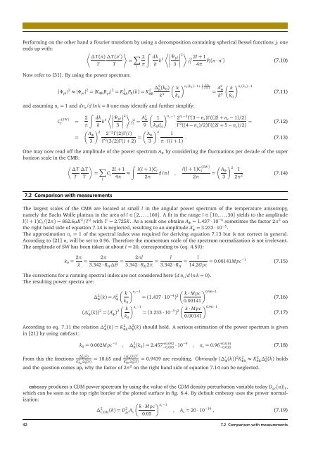
Performing on the other hand a Fourier transform by using a decomposition containing spherical Bessel functions jl one
ends up with:
�
∆T(n) ∆T(n
T
′ � �
) � 2 dk
=
T π k k3
�� �2
���Ψ
pl�
�
3�
�
j 2 2l+ 1
l 4π Pl(n· n ′ ) (7.10)
Now refer to [31]. By using the power spectrum:
|Ψpl| 2 ≈|Φ pl| 2 =|KΦRR pl| 2 = K 2
ΦRPR(k)=K 2
∆
ΦR
2
R (k0) k3 and assuming n s= 1 and dn s/d ln k=0 one may identify and further simplify:
C (SW)
l
= 2
�
dk
π
=
k k3
�� 2
AΦ
3
�� ���
Ψ pl
3
�
�
�
�
2 �
j 2
l
l
= A2
Φ
2 −2 Γ(2)Γ(l)
Γ 2 (3/2)Γ(l+ 2) =
9
� k
k 0
�ns(k0)−1+ 1 dns
2 d ln k
= A2
Φ
k3 �� ns(k
k 0)−1
k0 (7.11)
� �ns−1 n 1 2 s−3Γ(3− ns)Γ((2l+ ns− 1)/2)
k0dA Γ2 = (7.12)
((4− ns)/2)Γ((2l+ 5− ns)/2) �� 2
AΦ
3
1
. (7.13)
π·l(l+ 1)
One may now read off the amplitude of the power spectrum A Φ by considering the fluctuations per decade of the super
horizon scale in the CMB:
� �
∆T ∆T � 2l+ 1
= Cl T T
4π ≈
�
l(l+ 1)Cl
d ln l ,
2π
7.2 Comparisonwith measurements
l
l(l+ 1)C (SW)
l
2π
=
� AΦ
3
� 2 1
2π 2
(7.14)
The largest scales of the CMB are located at small l in the angular power spectrum of the temperature anisotropy,
namely the Sachs Wolfe plateau in the area of l∈[2, . . ., 100]. A fit in the range l∈[10, . . ., 30] yields to the amplitude
l(l+ 1)Cl/(2π)=862.6µK 2 /T 2 with T= 2.725K. As a result one obtains AΦ= 1.437·10 −4 sometimes the factor 2π 2 on
the right hand side of equation 7.14 is neglected, resulting to an amplitude A ′
Φ = 3.233·10−5 .
The approximation ns= 1 of the spectral index was required for deriving equation 7.13 but is not correct in general.
According to [21] ns will be set to 0.96. Therefore the momentum scale of the spectrum normalization is not irrelevant.
The amplitude of SW has been taken at about l= 20, corresponding to (eq. 4.59):
k 0= 2π
λ =
2π
3.342·R H∆θ =
2πl
3.342·R H2π =
l l
= = 0.00141M pc−1
3.342·R H 14.2Gpc
The corrections for a running spectral index are not considered here (d n s/d ln k=0).
The resulting power spectra are:
∆ 2
�
k
Φ (k)= A2
Φ
(∆ ′
Φ (k))2 =(A ′
Φ )2
According to eq. 7.11 the relation∆ 2
Φ
in [21] by usingcmbfast:
�ns−1 =(1.437·10 −4 ) 2
�
k· M pc
k0 �ns−1 =(3.233·10
k0 −5 ) 2
� k
(k)= K2
k 0= 0.002M pc −1
ΦR∆2 R
0.00141
�
k· M pc
0.00141
� 0.96−1
� 0.96−1
(7.15)
(7.16)
(7.17)
(k) should hold. A serious estimation of the power spectrum is given
, ∆ 2
R (k0)= 2.457 +0.092
−0.093 · 10−9
, n s= 0.96 +0.014
−0.013
From this the fractions ∆2
Φ (k)
K2 Φ ∆
R 2
(∆′ Φ
R (k)=
18.65 and (k))2
K2 ΦR∆2 R (k)=
0.9439 are resulting. Obviously(∆′ Φ (k))2K 2
ΦR≈ K2
and the question comes up, why the factor of 2π2 on the right hand side of equation 7.14 can be neglected.
ΦR∆2 R
(7.18)
(k) holds
cmbeasy produces a CDM power spectrum by using the value of the CDM density perturbation variable today Dgc(a)| 1,
which can be seen as the top right border of the plotted surface in fig. 6.4. By default cmbeasy uses the power normalization:
∆ 2
C DM (k)= D2
gcAs � k· M pc
0.05
� ns−1
, A s= 20·10 −10 , (7.19)
42 7.2 Comparison withmeasurements