Master Thesis

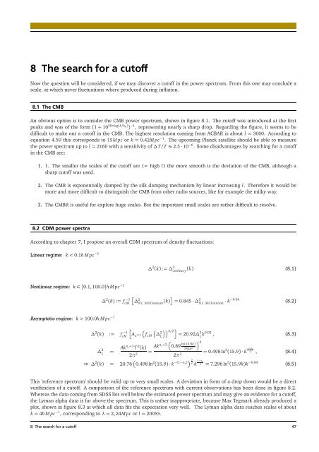
8 The search for a cutoff
Now the question will be considered, if we may discover a cutoff in the power spectrum. From this one may conclude a
scale, at which never fluctuations where produced during inflation.
8.1 The CMB
An obvious option is to consider the CMB power spectrum, shown in figure 8.1. The cutoff was introduced at the first
peaks and was of the form(1+10 50∗log(k/k 0) ) −1 , representing nearly a sharp drop. Regarding the figure, it seems to be
difficult to make out a cutoff in the CMB. The highest resolution coming from ACBAR is about l= 3000. According to
equation 4.59 this corresponds to 15M pc or k=0.42M pc −1 . The upcoming Planck satellite should be able to measure
the power spectrum up to l= 2160 with a sensitivity of∆T/T≈ 2.5·10 −6 . Some disadvantages by searching for a cutoff
in the CMB are:
1. 1. The smaller the scales of the cutoff are (= high l) the more smooth is the deviation of the CMB, although a
sharp cutoff was used.
2. The CMB is exponentially damped by the silk damping mechanism by linear increasing l. Therefore it would be
more and more difficult to distinguish the CMB from other radio sources, like for example the milky way.
3. The CMBR is useful for explore huge scales. But the important small scales are rather difficult to resolve.
8.2 CDM power spectra
According to chapter 7, I propose an overall CDM spectrum of density fluctuations:
Linearregime: k100.0h M pc −1
∆ 2 (k) :=∆ 2
cmbeas y (k) (8.1)
∆ 2 (k) := f −1
�
2
cM ∆N L Millennium (k)� = 0.845·∆ 2
N L Millennium · k−0.04
∆ 2 (k) := f −1
� �
cM Ax 3/2 fcM
∆ 2
L
= Akn s+3 T 2 (k)
2π 2
=
��� �
2
3/2
∆L Ak n s+3
�
(8.2)
= 20.92∆ 3
L k0.02 , (8.3)
0.89 ln(15.9k)
783k 2
2π 2
⇒ ∆ 2 (k) = 20.76 � 0.498 ln 2 (15.9)·k −(1−n s)
� 3
� 2
= 0.498 ln 2 (15.9)·k 1−ns
2 , (8.4)
2 k 1−ns
2 = 7.296 ln 3 (15.9k)k −0.04
This ’reference spectrum’ should be valid up to very small scales. A deviation in form of a drop down would be a direct
verification of a cutoff. A comparison of the reference spectrum with current observations has been done in figure 8.2.
Whereas the data coming from SDSS lies well below the estimated power spectrum and may give an evidence for a cutoff,
the Lyman alpha data is far above the spectrum. This is rather inappropriate, because Max Tegmark already produced a
plot, shown in figure 8.3 at which all data fits the expectation very well. The Lyman alpha data reaches scales of about
k= 4h M pc −1 , corresponding toλ=2, 24M pc or l= 20055.
8 The searchfor a cutoff 47
(8.5)