Master Thesis

dn(M) / dlog M [(h −1 Mpc) −3 ]
10 16
10 15
10 14
10 13
10 12
10 11
10 10
10 9
10 8
M −1
10 −6 10 −5 10 −4 10 −3 10 −2 10 −1 10 0 10 1
M [h −1 M ]
solar
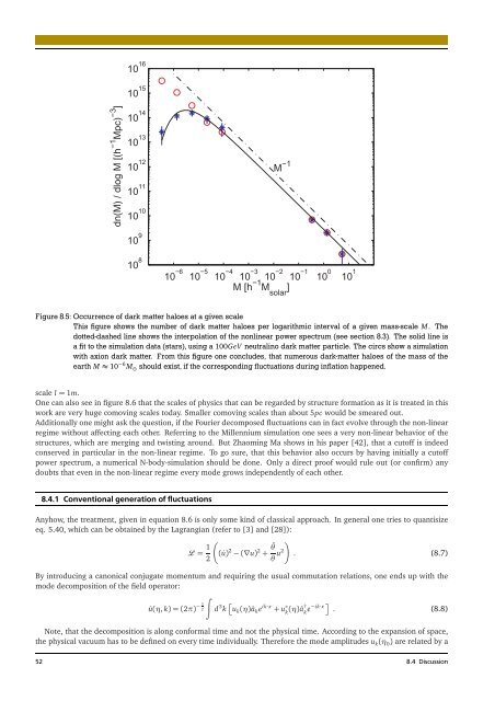
Figure8.5: Occurrenceof darkmatter haloes at a given scale
This figure shows the number of dark matter haloes per logarithmic interval of a given mass-scale M. The
dotted-dashed line shows the interpolation of the nonlinear power spectrum (see section 8.3). The solid line is
afit tothe simulation data(stars), usinga100GeV neutralino darkmatter particle. The circsshow a simulation
with axion dark matter. From this figure one concludes, that numerous dark-matter haloes of the mass of the
earth M≈ 10 −6 M ⊙ should exist,if the correspondingfluctuations duringinflation happened.
scale l= 1m.
One can also see in figure 8.6 that the scales of physics that can be regarded by structure formation as it is treated in this
work are very huge comoving scales today. Smaller comoving scales than about 5pc would be smeared out.
Additionally one might ask the question, if the Fourier decomposed fluctuations can in fact evolve through the non-linear
regime without affecting each other. Referring to the Millennium simulation one sees a very non-linear behavior of the
structures, which are merging and twisting around. But Zhaoming Ma shows in his paper [42], that a cutoff is indeed
conserved in particular in the non-linear regime. To go sure, that this behavior also occurs by having initially a cutoff
power spectrum, a numerical N-body-simulation should be done. Only a direct proof would rule out (or confirm) any
doubts that even in the non-linear regime every mode grows independently of each other.
8.4.1 Conventionalgenerationoffluctuations
Anyhow, the treatment, given in equation 8.6 is only some kind of classical approach. In general one tries to quantisize
eq. 5.40, which can be obtained by the Lagrangian (refer to [3] and [28]):
�= 1
�
(˙u)
2
2 −(∇u) 2 ¨θ
+
θ u2
�
. (8.7)
By introducing a canonical conjugate momentum and requiring the usual commutation relations, one ends up with the
mode decomposition of the field operator:
�
3
−
û(η, k)=(2π) 2
d 3 k � u k(η)â ke ik·x + u ∗
k (η)â†
k e−ik·x� . (8.8)
Note, that the decomposition is along conformal time and not the physical time. According to the expansion of space,
the physical vacuum has to be defined on every time individually. Therefore the mode amplitudes u k(η 0) are related by a
52 8.4 Discussion