Robert van Geldern, Johannes A.C. Barth. 2012. Optimization of ...

LIMNOLOGY 

and 

OCEANOGRAPHY: METHODS 

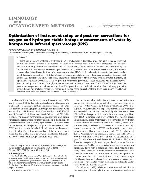
Optimization of instrument setup and post-run corrections for 

oxygen and hydrogen stable isotope measurements of water by 

isotope ratio infrared spectroscopy (IRIS) 

Robert van Geldern * and Johannes A.C. Barth 

GeoZentrum Nordbayern, University of Erlangen-Nuremberg, Schlossgarten 5, 91054 Erlangen, Germany 

Abstract 

Light stable isotope analyses of hydrogen ( 2H/ 1H) and oxygen ( 18O/ 16O) of water are used in many terrestrial 

and marine aquatic studies. The advantage of using stable isotope ratios is that water molecules serve as ubiquitous 

and already present natural tracers. Within recent years, these analyses have been revolutionized by the 

development of new isotope ratio laser spectroscopy (IRIS) systems that are cheaper, more robust, and mobile 

compared with traditional isotope ratio mass spectrometry (IRMS). Although easier to operate, laser systems also 

need thorough calibration with international reference materials, and raw data need correction for analytical 

effects (i.e., memory and drift). This study presents modifications to the hardware for liquid water injection, an 

optimized sequence layout and a simple post-run correction procedure. These protocols will maximize precision, 

accuracy, and sample throughput via an efficient memory correction. The number of injections per 

unknown sample can be reduced to 4 or less. This procedure meets the demands of faster throughput with 

reduced costs per analysis. Procedures presented here are based on real analyses. They were also verified by an 

international proficiency test and traditional IRMS techniques. 

Analyses of the stable isotope composition of oxygen (d 18 O) 

and hydrogen (d 2 H) in the water molecule are a widespread and 

established tool in many scientific disciplines. They are of particular 

interest in oceanography, limnology, and hydrology (Craig 

and Gordon 1965; Benson 1994; Clark and Fritz 1997; Kendall 

and McDonnell 1998; Pham et al. 2009; Schulte et al. 2011). For 

instance, the isotope composition of precipitation and surface 

water has been monitored for many decades on a global scale by 

the International Atomic Energy Agency (IAEA) in Vienna in the 

Global Network of Isotopes in Precipitation (GNIP) (IAEA/WMO 

2006) and the recently launched Global Network of Isotopes in 

Rivers (GNIR). The isotope composition of the oceans is documented 

in the Global Seawater Oxygen-18 Database (Schmidt et 

al. 1999), starting with isotope data from about 1950. 

*Corresponding author: E-mail: robert.v.geldern@gzn.uni-erlangen.de 

(R. van Geldern), barth@geol.uni-erlangen.de (J.A.C. Barth). 

Tel.: + 49 9131 8522514; fax: + 49 9131 29294 

Acknowledgments 

We thank Silke Meyer and Irene Wein (Erlangen), who helped with 

laboratory work. Partial financial support was provided by institutional 

grants from the Bavarian government for climate protection and by 

funds for instrumentation for the chair of Applied Geology at the 

GeoZentrum Nordbayern. We thank two anonymous reviewers for their 

helpful comments. 

DOI 10.4319/lom.2012.10.1024 

1024 

Limnol. Oceanogr.: Methods 10, 2012, 1024–1036 

© 2012, by the American Society of Limnology and Oceanography, Inc. 

For many decades, stable isotope analyses of water were 

exclusively performed by so-called isotope ratio mass spectrometry 

(IRMS) (Werner and Brand 2001; Brand 2004). During 

the 1990s, the classical high vacuum dual inlet technique 

was extended, and in parts, replaced by the continuous flow 

(CF-IRMS) technique, which uses helium as a carrier gas. However, 

IRMS technique can only analyze the gaseous phase. 

Consequently, liquid water has to be converted to hydrogen 

for d 2 H analysis by reduction with hot (~800°C) metals (i.e., 

uranium, zinc, or chromium). In continuous flow mode, high 

temperature pyrolysis (>1050°C) can be used to convert water 

to hydrogen (d 2 H) and carbon monoxide (d 18 O) (Gehre et al. 

2004). Alternatively, equilibration techniques with CO 2 for 

d 18 O (Epstein and Mayeda 1953) or with H 2 by platinum catalysts 

for d 2 H (Ohsumi and Fujino 1986; Horita 1988) exist. 

These techniques apply various peripheral units to the mass 

spectrometer. Stable isotope ratio mass spectrometers are 

expensive, have high operational costs, and require a relatively 

large space in climate-controlled laboratories. Field 

operation with direct in situ analysis of water samples is not 

possible. On the other hand, despite these disadvantages, 

IRMS has performed high-precision and accurate isotope measurements 

over decades, which significantly helped to understand 

earth and aquatic processes. 

Kerstel et al. (1999) published a new method, which uses 

the absorption of laser light for the simultaneous analyses of

van Geldern and Barth Water stable isotope analysis with IRIS 

d 18 O and d 2 H in water vapor. During the last years, this technique 

was improved (Kerstel and Gianfrani 2008) and new 

commercially available instruments entered the analytical 

market. This technique is referred to as stable isotope ratio 

infrared spectroscopy (SIRIS or IRIS in the more recent literature; 

Chesson et al. 2010). The developers and manufacturers 

of these instruments highlight some major advantages over 

the traditional IRMS technique. The IRIS method allows direct 

measurement of water vapor with almost no sample preparation. 

Laser-based instruments are cheaper and can be built in 

a compact and lightweight design for in situ and real-time 

monitoring applications. A number of studies showed that the 

new IRIS technique yields comparable precision and accuracy 

to traditional IRMS (Lis et al. 2008; Gupta et al. 2009; Chesson 

et al. 2010; Penna et al. 2010). However, it must be noted that 

this method is sensitive to organic contaminations (e.g., alcohol) 

in the sample, which may result in wrong analytical 

results (Brand et al. 2009). To detect such samples, Picarro Inc. 

offers an additional software tool (ChemCorrect TM ) that identifies 

potentially contaminated samples to the user. 

The new laser instruments opened possibilities for analyses 

of water stable isotopes to laboratories and users that are not 

familiar with classic isotope ratio analyses and the specific calibration 

and post-run correction strategies that are typically 

associated with this analytical method. The crucial point for 

correct isotope data are the appropriate implementation and 

use of isotope-specific correction and normalization procedures. 

In many cases, the manufacturers of laser isotope ratio 

analyzers do not stress the need for such specific procedures. 

Therefore, just following the manufacturers’ instructions will 

often not result in high-precision stable isotope analyses. Furthermore, 

laboratories without IRMS are not able to verify and 

double-check their analytical methods with the new instrument. 

Whereas most isotope laboratories running traditional 

IRMS can adopt their existing procedures, the increasing 

amount of new laboratories without such expertise need easyto-follow 

methods that enable them to obtain high-precision 

isotope data by the IRIS technique. 

Various approaches have been used for raw data correction 

and calibration of isotope data from several peripherals (Nelson 

2000; Nelson and Dettman 2001; Werner and Brand 2001; 

Brooks et al. 2004; Gehre et al. 2004; van Geldern and Suckow 

2005; Paul et al. 2007; Schmid et al. 2010; Gröning 2011). The 

most common approach is data evaluation by spreadsheets 

and typically follows general principles that have been 

reviewed for example by Werner and Brand (2001). In addition, 

some laboratory information management systems 

(LIMS), as LIMS for Light Stable Isotopes (Coplen 2000) or Lab- 

Data (Suckow and Dumke 2001), also support the import of 

IRMS and IRIS raw data and offer the ability for further data 

processing. 

The objectives of this study are to suggest improvements of 

the hardware with respect to the factory setup of laser isotope 

analyzers using water injection and to highlight some major 

1025 

pitfalls associated with this type of new instruments. This 

includes an optimized procedure for raw data processing. A 

focus of this study is on memory effects that are among the 

major sources of error in water stable isotope analyses by liquid 

injection. Following the suggestions will enable users to 

increase the lifetime of consumables (e.g., syringes). At the 

same time, they will increase sample throughput, precision, 

and accuracy of the analyses. In this manner, faster and 

improved analytical results will lower the operational costs per 

sample. The usability is demonstrated by real world examples 

and includes an international round-robin test. 

Materials and procedures 

Commercially available IRIS instruments for water stable 

isotope analyses are produced by Picarro Inc. and Los Gatos 

Research Inc. (LGR). Trace gas analyzers based on the older 

lead-salt laser technology produced by Campbell Scientific 

Inc. are not available anymore but may still be in use for isotope 

water vapor measurements. Note that the protocols presented 

here (i.e., the memory correction scheme) were developed 

for liquid water injection by a vaporizer and cannot be 

directly applied to existing other or new sample introduction 

systems (e.g., Picarro induction module). In this study, a 

Picarro L1102-i WS-CRDS analyzer with vaporization module 

V1102-i coupled to a CTC PAL autosampler (CTC Analytics) 

has been used. All analyses were done in high precision mode. 

The results of the Picarro system were compared with traditional 

IRMS data, which were analyzed for d18O by an automated 

equilibration unit (Gasbench 2, Thermo Scientific) in 

continuous flow mode coupled to a Delta plus XP isotope ratio 

mass spectrometer. 

All values are expressed in the standard delta notation in 

per mil (‰) versus VSMOW according to 

(1) 

where R is the isotope ratio of the heavy and light isotope 

(e.g., 18O/ 16O) in the sample and the reference. The data were 

normalized to the VSMOW/SLAP scale by assigning a value of 

0‰ and –55.5‰ (d18O)/0‰ and –427.5‰ (d2 ⎛ ⎞ 

d = ⎜ − ⎟ 

⎝ ⎠ 

H) to VSMOW2 

and SLAP2, respectively. For data normalization, two laboratory 

reference waters that were calibrated directly against 

VSMOW2 and SLAP2 were measured in each run. 

The carry-over of residual amounts from one sample to the 

other, denoted as memory effect, is expressed as the measure 

of how close the measurement comes to its ideal (or true) 

value after a number of repeat injections. The associated memory 

coefficient m is defined here as 

(2) 

× 

Rsample 

1 1000 

Rreference 

( n−1) 

n 

n dt−di mi = ( n−1) 

n 

d −d 

t 

whereas i is the number of injection of sample n. The subscript 

t denotes the isotope value that is regarded as the true value of 

the sample. d t represents the value around which results stabi- 

t


lize after numerous injections. It is typically the value of the last 

injection or is calculated as an average from the last few injections. 

For example, a memory coefficient of 0.98 means that the 

analyzed isotope value represents 98% of the true isotope value 

of the sample. In other words, it is influenced by 2% from the 

precursor sample. This definition has the advantage that it is 

independent of the absolute difference in delta value of two 

adjacent samples. It is also independent of the direction of the 

change in delta values (positive or negative). 

Modifications to the analytical hardware 

After setup of the laser spectroscopy system, some modifications 

including a change of syringe type and number of 

injections compared with the original factory setup have been 

applied. This results in lower analytical costs and increased 

analytical performance as well as higher sample throughput. 

An overview of all modifications is provided in Table 1. 

One critical point is the lifetime of the syringe that can 

become a major cost factor. The delivered and recommended 

5 µL syringe clogged fast and had to be replaced several times 

per month. It was exchanged with a more robust and cheaper 

10 µL model (SGE Analytical Science; alternative: Hamilton 

Bonaduz AG). The injection volume remained unchanged at 

1.8 µL, which yielded a signal height of about 20.000 ppmV 

H 2 O after vaporization. The reproducibility of the injection 

volume with the 10 µL syringe was identical to the 5 µL 

Table 1. Picarro factory setup versus modifications in the Erlangen stable isotope laboratory. 

1026 

model. Additionally, a daily manual clean-up of the plunger 

with N-Methyl-2-pyrrolidone (NMP, technical grade) helped 

to significantly increase the syringe lifetime and to reduce 

analytical costs. For manual cleaning, it is crucial to take out 

the plunger completely and to clean the entire body. This is 

important because the uppermost part of the syringe and 

plunger has been identified as the main source of error. This 

part of the syringe is usually not reached by the automatic 

wash cycle of the auto sampler and can accumulate crusts, 

which will block the plunger. In case of persistent crusts, the 

syringe can be placed into an ultrasonic bath with deionized 

water before NMP cleaning. Note that increasing the number 

of post-injection wash cycles or use of combinations of solvents 

did not help to keep the plunger running smooth. 

Therefore, there is currently no alternative to regular manual 

cleaning. 

For isotope measurements, it is important to prevent evaporation 

of the water sample. During the sequence run (typical 

up to 24 h), some water will evaporate into the vials headspace 

and may subsequently leave via a loose cap. Consequently, 

the remaining liquid water becomes enriched in the 

heavy isotope relative to the water vapor due to a Rayleigh 

fractionation process. Therefore, the 1.5 mL standard GC vials 

used in the CTC autosampler must have caps with tight fit. 

This is crucial for very low sample volumes and the use of 

Parameter Picarro Inc. factory setup 

Modification at Erlangen 

stable isotope laboratory Observation 

Syringe 5 µL SGE (#001982) 10 µL SGE (#002980) 

10 µL Hamilton (#203205/02) 

increased syringe lifetime 

Vials delivered with Fisher-brand ® vials, 

caps with PTFE/silicon septa 

Filling volume of 

autosampler vials 

Agilent type 1.5 mL vials (thread N9-425); caps 

with PTFE/red rubber septa (VWR #548-0907) 

Fisher-brand ® caps had bad fit on 

thread and were leaky 

no recommendation 800 µL High liquid to headspace ratio 

minimizes evaporation effects 

Injection volume 1.8 µL 1.8 µL (no modification) 

Needle rinse 2 pre-injection cleanings with 

sample 

Wash cycles no recommendation; NMP * is suggested 

Memory correction no correction, ignore first 3 injections 

2 pre injection cleanings with sample (no modification) 

Fresh water: one post-injection wash cycle with 

NMP 

Salt water: one additional wash cycle with DI 

water before NMP 

mathematical memory correction based on standard 

injections 

Nr of injections 6 reference waters: 10 samples: 4 (no injection 

ignored) 

Injection port septa Restek 3 / ” IceBlue 8 ® (#27159) 

general-purpose septa; had to be 

3 

/8 ” ‘Marathon’ long-life silicon septa, from CS- 

Chromatographie Service, Germany (#366082); 

replaced daily (lifetime ~250 inj.) replaced weekly (lifetime > 600 injections) 

increased syringe lifetime 

no injection has to be ignored 

reduced nr of injections for samples, 

higher sample throughput 

lower maintenance, increased lifetime 

of the septa; allows for long 

sequences over weekends 

Other 

Daily manual cleaning of syringe plunger with NMP increased syringe lifetime 

* N-Methyl-2-pyrrolidone (CAS No: 872-50-4)


micro inserts. For standard analysis, a filling volume of 800 µL 

is recommended. This minimizes any evaporative effect below 

analytical precision. Septa with good re-sealing characteristics 

should be used for analyses with multiple injections. Typical 

combinations with such characteristics are PTFE/silicon or 

PTFE/rubber septa. The filling of the vials with samples and 

reference waters should be carried out immediately before the 

start of the sequence. Prefilling of autosampler racks with samples 

or reference waters and storage overnight is not recommended. 

Also, the reuse of vials with reference waters in the 

next sequence yielded unreliable results and should be 

avoided. 

Sequence layout 

The number of injections needed per sample is one of the 

most important issues with respect to sample throughput and 

analytical costs. Furthermore, the general layout of a 

sequence, i.e., the number and position of reference waters 

and the number of injections has to meet the needs of postrun 

corrections applied to the raw data. Post-run corrections 

applied in isotope analyses depend on the specific characteristics 

of the sample preparation device. Typical applied corrections 

are (1) linearity, (2) sample-to-sample memory, and (3) 

drift. Finally, the corrected data set is normalized to the 

VSMOW/SLAP scale by assigning calibrated values to two inhouse 

reference waters. 

Linearity corrections for IRMS are instrument dependent 

and are machine specific (Werner and Brand 2001; Barth et al. 

2004). The injection volume for the IRIS system is kept constant, 

which gives a constant signal height in the detector. 

Therefore, linearity effects of the detector can be neglected. 

An optimized standard sequence is shown in Fig. 1. The 

scheme was arranged to fulfill the needs of corrections (2) and 

(3) and the subsequent normalization to the international 

scale. The sequence uses four in-house reference waters 

(Table 2). These were calibrated directly against primary international 

reference materials (VSMOW2, GISP, and SLAP2) that 

are distributed by the Reference Products for Environment and 

Trade section of the IAEA, Vienna, or the National Institute of 

Standards and Technology (NIST). Run times of the sequences 

are typically less than 24 h to allow for the daily maintenance 

of the equipment (syringe cleaning, etc.) and data evaluation 

to identify potential problems before the preparation and start 

of the next sequence. 

The sequence uses the “high precision” mode of the instrument 

and begins with the injection of the drift-monitoring 

water (DEST, Table 2 and Fig. 1). The number of injections is 

set to 10, whereas the first 3 to 6 injections serve as “warm 

ups” for the instrument and are ignored for any further data 

evaluation. Injections 7 to 10 serve as the first anchor for the 

drift correction function. Other data points for this correction 

are drawn from the repeat analyses of the DEST reference 

water that is distributed regularly over the sequence (vials nr 

9, 18, and 27 in Fig. 1). Injections of the references are always 

performed from a separate vial for three reasons: 

1027 

(1) The re-injection from a single vial will puncture the septa 

several times and the waters can be enriched by evaporation 

through leaking septa. The isotope values will shift to 

higher numbers over time. This can be wrongly interpreted 

as instrument drift. 

(2) The filling and analysis of individual vials yield better values 

of the analytical reproducibility throughout a 

sequence, because it includes errors and variations from 

sample preparation. 

(3) The autosampler programming is much faster with this 

type of setup and can be edited more easily at the CTC 

touchpad. 

The next step is the injection of three isotopically different 

waters (named HIS, ANTA, and HERA, see Table 2) with high, 

low, and intermediate values. The difference in isotope compositions 

results in a distinct sample-to-sample carry over 

that is clearly visible in these successive injections. This is 

used to calculate memory coefficients on a daily basis for further 

data evaluation. The low and high reference waters are 

also used to normalize the data to the VSMOW/SLAP scale 

after memory and drift correction. The isotope composition 

of the fourth isotope reference water is chosen to be close to 

the expected values of the usually analyzed samples in the 

laboratory (here: Central European fresh water) and is treated 

as a sample with unknown isotope ratio. It is not used to 

establish any correction function and serves as an independently 

prepared quality control (QC) sample. By recording the 

results of the QC sample from day to day, this sample is used 

to examine the daily accuracy of analyses, and to monitor the 

long-term precision. 

Memory correction 

Depending on the difference in isotope values between two 

samples, the first injections of the successive vial are influenced 

by the precursor. The values of successive injections 

approach a stable isotope value after a certain number of injections. 

This number of injections needed for a stable value 

depends on the amplitude of the memory effect, which in 

turn, depends on the instrument’s design and the magnitude 

of the isotope difference between samples. Tests indicated that 

syringe-type or numbers of cleaning cycles are only of minor 

importance for the amplitude of the memory effect. Additional 

post injection cleaning cycles with DI water and/or 

NMP did not reduce the observed memory effect. Therefore, 

the major source of the memory effect seems to be related to 

the injection port. In traditional IRMS, practically memoryfree 

systems such as water equilibration with gaseous CO 2 or 

H 2 are available. Other systems with direct conversion of the 

water sample, such as the reduction of H 2 O to H 2 by hot 

chromium (Thermo Scientific H/Device) or conversion to H 2 

and CO by high temperature pyrolysis show a memory in the 

range of 2% or less for the first injection (m 1 = 0.98) (Werner 

and Brand 2001; Gehre et al. 2004). In case of the high temperature 

pyrolysis, the memory effect could be reduced by 

modifications to the gas flow (Gehre et al. 2004).


Fig. 1. Typical sequence layout with 27 positions (high precision mode) with four reference waters with 10 injections at the beginning. HIS and ANTA 

are the names of reference waters with high and low delta values used for scale normalization (Table 2). DEST and HERA are intermediate waters, whereas 

DEST is used for drift monitoring and HERA (Vial nr 5) is treated as sample for quality control. Vials nr 2, 3, and 4 are used to calculate memory correction 

factors (see text). 

In contrast to this, possible changes to the Picarro vaporizer 

module are limited to septa material, syringe type, injection and 

cleaning parameters, and temperature. Changes in these parameters 

had no or negligible influence on the memory effect. The 

1028 

number of injections needed on the IRIS system for a reliable 

isotope value is crucial for sample throughput and directly 

related to the costs per sample. The main possible approaches to 

reduce memory effects can be summarized as follows:


Table 2. Laboratory reference materials. 

Name Type Purpose Source 

VSMOW2/GISP/SLAP2 International reference material Calibration of in-house reference waters distributed by IAEA and NIST * 

In-house waters: HIS high isotope water (d18O: –1.31/d2H: –7.4) Normalization to VSMOW/SLAP scale Sea water, deionized 

ANTA low isotope water (d18O: –32.81/d2H: –259.8) Normalization to VSMOW/SLAP scale Antarctic snow, deionized 

DEST intermediate water (d18O: –8.82/d2H: –63.3) Drift monitoring Erlangen tap water, deionized 

HERA intermediate water (d18O: –6.18/d2H: –53.6) Quality control standard; treated as sample Erlangen tap water, deionized 

Memory correction is calculated from subsequent injections of HIS, ANTA, and DEST 

* Online catalogues can be accessed at http://nucleus.iaea.org/rpst/index.htm (IAEA) and http://www.nist.gov/srm/index.cfm (NIST). 

(1) Ignore the first injection(s) of a sample and calculate the 

final value from the last injections after stabilization of the 

isotope value. In its standard setup, Picarro Inc. recommends 

performing 6 injections per sample, ignoring the 

first 3 injections, and averaging the final value from the last 

3 injections. This results in large numbers of injections per 

sample that have to be discarded, and thus, creates analytical 

costs. Furthermore, in many cases, the number of 6 

injections per sample is clearly insufficient to reach a stable 

isotope value for d 2 H (Fig. 2). The size of error depends on 

the magnitude of the difference in isotope composition 

between two samples. Therefore, by following this procedure, 

analytical results may suffer from memory effects. 

This is especially true for the isotope reference waters with 

high and low d-values that serve for normalization to the 

VSMOW/SLAP scale. Correct analysis of these references is 

essential for high-precision stable isotope values and 

ensures comparability of data between laboratories. 

(2) A mathematical memory correction based on the influence 

of the previous sample and the sample(s) before. This 

approach has been successfully applied to systems with 

low memory effects, such as the Thermo Scientific 

H/Device. In these systems, the isotope value typically stabilizes 

after 3 or 4 injections. A prerequisite for this 

approach is that each sample is injected often enough 

until the value is stable. The mathematical correction only 

eliminates the need to discard the first injections. The final 

value can then be averaged from all injections. 

(3) Create a static memory correction table based on “memory 

runs.” In these runs, waters with large differences in isotope 

values are analyzed numerous times in alternating 

sequential arrangement with a sufficient high number of 

injections for each sample (typically 15 to 20 injections). 

The average memory coefficients for the injections are 

stored in a table, and are used in further sequences for a 

mathematical memory correction of the analytical results. 

This allows for a reduction to 3 or 4 injections per sample. 

Templates of Bruce Vaughn from the stable isotope laboratory 

of the Institute of Arctic and Alpine Research 

(INSTAAR), University of Colorado have been provided by 

courtesy of Picarro Inc. upon request. This approach works 

well as long as the memory coefficients do not change. As 

1029 

Fig. 2. Memory effect on the (A) d 18 O and (B) d 2 H value of the injections 

of a sample analyzed after a sample with a large difference in isotopic 

composition (dΔ). 

shown below, the memory coefficient is not necessarily 

stable over time and may depend on the sample matrix 

(e.g., salinity, alkalinity, pH, etc.). A change in sample 

matrix always bears the risk of an undetected change of 

the memory coefficients. To ensure appropriate and up-todate 

memory coefficients, frequent repetitions of these 

time-consuming runs have to be carried out. 

(4) In this study, we suggest a memory correction approach 

based on the daily analysis of multiple reference waters 

that are already incorporated in each sequence for normalization 

to the SMOW/SLAP scale. After a fast and simple 

iterative determination of memory coefficients at the


beginning of each sequence, these coefficients can be 

applied to all subsequent injections of the sequence. This 

ensures use of up-to-date memory coefficients for mathematical 

memory corrections. Theoretically, after the initial 

multiple injection of the reference waters one injection per 

sample would be sufficient. However, to allow for appropriate 

statistical calculations a minimum of 4 injections 

per sample is recommended. This correction approach is 

described in more detail in the following section. 

Calculation of memory coefficients 

For analyses of two adjacent samples with a large difference 

in their delta values, the number of injections required to 

obtain a sufficiently stable value needs to be determined. The 

maximum differences in delta values (Δd) occur between the 

low and high reference waters. For the in-house reference 

waters used in this study the maximum Δd values are 31.5‰ 

(d 18 O) and 252‰ (d 2 H), respectively (Fig. 1, Table 2). This 

range usually covers most of the naturally occurring samples, 

except for some ice core samples or samples from extreme 

environments such as deserts or polar regions. 

The number of injections necessary to obtain a stable value 

for the correction procedure can be determined from Fig. 2. 

For the oxygen isotope composition (d 18 O) the raw delta value 

is within the range of the generally cited analytical uncertainty 

of 0.1‰ after 5 to 7 injections. For hydrogen, the situation 

is different and 10 to 12 injections are needed to 

securely reach the 1‰ corridor around a steady value. This is 

typically regarded as the analytical uncertainty for d 2 H. It must 

be noted here that the number of injections needed for a stable 

isotope value depends on the absolute difference dΔ 

between two samples. For a larger dΔ (427.5‰ in d 2 H for 

VSMOW2 and SLAP2), the number of injections for a stable 

value can be significantly higher (Gröning 2011). The number 

of repeat injections has to be evaluated for the used laboratory 

reference waters. For the following calculation of the memory 

coefficients, we determined that the necessary stable value 

within the analytical uncertainty is achieved after ten injections. 

This is definitely true for d 18 O, whereas it is a practical 

compromise for d 2 H. Numerous tests indicated that no further 

analytical accuracy and precision is gained for a dΔ of 24‰ to 

34‰ (d 18 O) and 196‰ to 252‰ (d 2 H) with more than 10 

injections of the three in-house reference waters. 

In principle, the memory coefficients can be calculated by 

using only one pair of reference waters. This, however, results 

in a poor correction of the other reference waters because no 

statistical variations of the raw data are considered. By using 

three successive injections, the full range of small and large Δd, 

as well as positive and negative changes, are taken into 

account. The laboratory reference water with the most positive 

isotope value is named HIS, the most negative is named 

ANTA, and the intermediate water is named DEST (Table 2). 

Three successive injections of DEST to HIS, HIS to ANTA, and 

ANTA to DEST were used for the determination of the memory 

coefficients (see Fig. 1 for dΔ amplitudes). The sample stan- 

1030 

dard deviation (s.d.) of the ten injections of each vial is calculated 

for HIS (vial nr 2), ANTA (nr 3), and DEST (nr 4). The 

standard deviation of the raw delta values without memory 

correction is large (>0.2‰ for d 18 O and >3‰ for d 2 H) due to 

the influence of the previous sample on the first injections 

(see Fig. 2). The weighted mean of the combined standard 

deviation (c.s.d.) is calculated according to: 

2 

csd .. . = (. sd.) n 

i 

∑ 

n= 

1 

with (s.d.) 2 being the variance of all injections i of vial number 

n. The variance is defined as the square of the standard deviation. 

Using the variance instead of the standard deviation 

results in a larger influence of the large isotopic shifts (Δd) 

whereas smaller shifts assume a lesser weight in the calculated 

c.s.d. This weighted approach takes into account that for a 

small Δd between two successive samples, the delta values of 

the first injections are influenced less by the previous vial 

compared with larger differences between samples. In other 

words, samples that have a larger memory effect are considered 

to a larger extent. 

For the analyses of real environmental samples, the isotope 

values typically group in narrow ranges for a specific type of 

sample and often do not show extreme dΔ changes from one 

sample to the other. The weighted approach according to Eq. 3 

also efficiently hampers the “overcorrection” of an injection. 

This problem often becomes obvious in analyses of real world 

samples by using an unweighted approach or a simple arithmetic 

mean for the determination of the memory coefficients. 

The determination of the memory coefficients m 1 to m 10 is 

performed by the “solver” function of Microsoft Excel. This 

starts an iterative process with the constraint to minimize the 

c.s.d value. There is no mathematical function fitted to the 

memory coefficients. The program varies the numbers for the 

coefficients in order to find values that yield a minimum value 

for c.s.d. The presettings for the solver function are specified as 

follows: (1) Constraint: minimization of c.s.d.; (2) no correction 

for last injection: m 10 = 1.0. This assumes that the last injection 

is the best representative of the true isotope value d t ; (3) m is 

monotonically increasing or remains identical: m i ≥ m i – 1. This 

means the memory effect becomes smaller from one injection 

to the next. When a stable value is reached m does not change 

anymore; (4) for all memory coefficients: m i ≤ 1.0. There will be 

no value larger than 1, which already means no memory. 

After correction, the c.s.d and the s.d. of the reference 

waters are minimal, and a linear regression through the memory 

corrected isotope values of all injections of a vial should 

have a slope of close to zero (Fig. 3). 

The determined memory coefficients m i now can be used to 

correct the raw delta values of the analyzed samples. After this 

correction, all injections can be used to calculate the arithmetic 

average, and no injections have to be discarded. With 

this, the number of injections for samples can be significantly 

reduced, because it is not necessary anymore to wait for the 

(3)


Fig. 3. Effect of the memory correction described in the text on the raw 

delta values of the three in-house reference waters (HIS, ANTA, DEST). All 

injections of a sample can be used after correction; no injection has to be 

discarded. Note that d-values are not scaled to the SMOW/SLAP scale. 

memory effect to fade away. The samples are injected 4 times 

in the standard sequence (Fig. 1). At the same time, the use of 

the memory correction increases accuracy and precision 

because the corrected values are not influenced by the previous 

sample, and all corrected values can be used. 

The memory-corrected values for injection i of a vial n are 

calculated according to 

n−1) 

memory corrected i ( raw ) i ( i( raw) 

t ) 

n 

n ( 

d = d + ( 1− 

m ) × d −d 

where m is the memory coefficient of the corresponding injec- 

i 

(n–1) tion number and d the true isotope value of the previous 

t 

sample. As the best approximation, d is set equal to the value 

t 

(4) 

1031 

Fig. 4. Memory coefficient of the first injection over time (shown interval 

is about 1 y). Usually only fresh water is analyzed. Seawater and brackish 

water were injected between 15-17 and 20-22 Jun 2011 (marked by 

vertical lines). The vaporizer was manually cleaned at 6 Mar 2012. 

of the last injection for the previous vial. The memory coefficient 

of the last injection (m 10 ) is set to 1.0 (see above). Therefore, 

the raw value is identical to the memory corrected value 

for this injection. 

Stability of memory coefficients over time 

Note that the memory effect may change over time. Fig. 4 

shows the calculated d 18 O memory coefficient for the first injection 

for about 1 year of analytical performance with 70 

sequences. The instrument mainly analyzed ground- and surface 

water samples, however two sets of seawater and brackish 

water were injected in June 2011. After these sequences, the 

matrix change of sample caused an increase of the memory 

effect. An increase of the sample-to-sample carry-over corresponds 

to a smaller number of the memory coefficient that 

dropped from values around 0.97 to values around 0.94. The 

main suspected process for this larger memory was salt deposition 

from seawater in the injection port of the vaporizer module. 

The subsequent injection of 10 sequences of fresh water 

samples between July and October did not change the memory 

coefficient, and it stayed around a value of 0.94. Note that this 

time period also coincided with a lesser frequency of sequences 

during the summer break. In October 2011, the memory effect 

of the first injection started to decrease, a fact that can be clearly 

seen by the rising numbers for m 1 in Fig. 4. The vaporizer had 

not been cleaned at this stage. The vaporizer was manually 

cleaned with deionized water on the 6 Mar 2011. Surprisingly, 

this procedure had hardly any noticeable influence on the 

memory effect. This one-year record emphasizes the need to use 

up-to-date memory coefficients for any mathematical correction 

of the raw data. This supports the procedure to determine 

the memory correction coefficients in each sequence.


Drift 

For drift monitoring, an in-house reference water (DEST) 

with an isotope value in the range of the usually analyzed 

samples is regularly re-analyzed in the sequence (Fig. 1). A 

nearly equidistant spacing of this interval is important for 

the correct calculation of a regression through the data. Also, 

the number of 4 injections is kept constant for each analysis 

of DEST. Otherwise, the regression would be influenced by 

the higher density of data points in one interval and may 

bias the drift over time. Therefore, the first 6 injections of 

DEST from position number 1 are ignored and are treated as 

“warm-up injections.” This number could be reduced in continuously 

running systems. However, after intervals, where 

the system has been shut off, up to 6 injections allow stabilization 

of both signal height and delta values. For drift correction, 

a linear regression is calculated from the memorycorrected 

data. The slope of the regression line applies to 

further correct the memory-corrected delta values as a function 

of time according to 

d drift corrected = d memory corrected + (slope × n) (5) 

where n is the position in the sequence that correlates to the 

analysis time. 

Typically, the system used in this study shows no or a small 

linear drift. For fresh waters the absolute change in mean dvalues 

between the first and last set of four injections of the 

drift reference water over 24 h is typically


Table 3. Comparison of d 18 O values (in ‰ versus VSMOW) analyzed on a memory free IRMS system by equilibration (Gasbench II) 

and Picarro IRIS data. The Picarro ran in high precision mode and data have been corrected by the scheme described in the text. Table 

is sorted by offset. 

LIMS ID Picarro (IRIS) * Gasbench (IRMS) † Offset 

W-1760 –9.06 –9.16 0.10 

W-1759 –8.98 –9.05 0.07 

W-1762 –8.89 –8.95 0.06 

W-1758 –9.25 –9.31 0.06 

W-1770 –5.33 –5.39 0.05 

W-1764 –0.59 –0.63 0.04 

W-1766 –1.49 –1.53 0.04 

W-1761 –8.72 –8.75 0.03 

W-1771 –2.88 –2.91 0.02 

W-1757 –9.37 –9.39 0.02 

W-1772 –4.42 –4.45 0.02 

W-1763 –2.87 –2.89 0.02 

W-1752 –9.05 –9.07 0.02 

W-1755 –9.22 –9.23 0.01 

W-1756 –9.23 –9.24 0.01 

W-1765 –1.99 –2.01 0.01 

W-1753 –9.16 –9.15 –0.01 

W-1769 –2.56 –2.55 –0.01 

W-1768 –1.92 –1.90 –0.02 

W-1774 –1.51 –1.49 –0.03 

W-1767 –0.61 –0.58 –0.03 

W-1773 –3.81 –3.77 –0.04 

W-1754 

* Mean value of four injections from one vial. 

† Mean value of two analyses from two vials. 

–9.23 –9.17 –0.06 

Table 4. Results of the IAEA-TEL-2011-01 proficiency test. The samples were analyzed in a routine sequence according to Fig. 1, and 

raw data were post-run corrected for memory and drift as described in the text. 

IAEA values * Reported value 

(all values in ‰ versus VSMOW) by Erlangen laboratory Offset 

d18O (± 2 s.d.) d2H (± 2 s.d.) d18O d2H d18O d2H Sample 1 0.39 (±0.04) –1.2 (± 0.4) 0.35 –1.2 –0.04 0.0 

Sample 2 –5.34 (±0.04) –43.3 (± 0.3) –5.38 –43.7 –0.04 –0.4 

Sample 3 –10.05 (±0.04) –72.9 (± 0.4) –10.03 –72.5 0.02 0.4 

Sample 4 –15.39 (±0.04) –114.0 (± 0.4) –15.42 –113.7 –0.03 0.3 

* Final report is not yet published by IAEA. Values are from IAEA’s official individual evaluation report. 

TEL-2011-01). Four unknown water samples were analyzed 

according to the scheme described in this study and raw data 

were processed with the correction procedures presented 

above. The samples were analyzed in a routine sequence. The 

reported results were within the analytical uncertainty given 

by the IAEA. Offsets between the reported and the true value 

were smaller than 0.05‰ for d 18 O and 0.5‰ for d 2 H (Table 4). 

Discussion 

The new laser-based IRIS systems have led to a significant 

increase in the number of laboratories performing iso- 

1033 

tope analyses over the last years. In addition, this technique 

is the first analytical equipment that can be operated 

outside the laboratory for real in situ measurements 

even in remote locations or on research vessels. This offers 

exciting new possibilities in various water-related research 

fields. Nonetheless, high accuracy and precision is still 

expected for results. In most cases, this conflicts with sample 

throughput, and sometimes, with environmental operational 

conditions. This study presents a detailed description 

that maximizes precision, accuracy and sample 

throughput.


Table 5. Gain in precision by applying the memory correction described in the text is demonstrated by the analysis of samples with 

a large difference in d-values. In-house reference waters HIS and ANTA were treated as unknown samples and analyzed in a standard 

sequence with 4 injections per vial on positions 6 and 7. Raw values were corrected for memory and drift and were normalized to the 

VSMOW/SLAP scale. Offset after corrections between analyzed and defined value is below 1‰ for d 2 H. All d-values are in per mil. 

d2H d2H d2H d2H d2Hmean Vial nr Inj. Nr Sample (raw) * (mem. corr.) (drift corr.) (norm.) (± 1 s.d.) d2Hdefined offset 

5 4 HERA –65.6 –65.5 –65.5 –54.3 

6 1 HIS –23.6 –18.7 –18.7 –7.9 –7.9 (± 0.2) –7.4 –0.5 

6 2 HIS –20.4 –18.9 –18.8 –8.1 

6 3 HIS –19.3 –18.4 –18.4 –7.6 

6 4 HIS –19.5 –18.9 –18.9 –8.1 

7 1 ANTA –247.2 –273.7 –273.6 –260.4 –260.3 (± 0.1) –259.8 –0.5 

7 2 ANTA –265.1 –273.4 –273.3 –260.1 

7 3 ANTA –269.0 –273.5 –273.5 –260.3 

7 4 ANTA –270.7 –273.6 –273.5 –260.3 

* Note that d-values of raw data depend on the user defined slope and intercept in the Picarro software. See instrument manual for editing these entries. 

The intention of this study was to present (1) modifications 

of the hardware, and (2) an optimized, easy-to-follow protocol 

for sequence layout and data evaluation. 

Proposed hardware modifications will significantly increase 

syringe lifetime, even with the analysis of problematic waters 

as saline brines. Memory corrections presented here are based 

on the actual measured data in the analytical sequence. With 

this, they also account for potential variations in the memory. 

The number of injections per unknown sample can be reduced 

to 4 or less injections per sample vial. This means that unnecessary 

injections that will be ignored at a later stage are not 

needed anymore. It, therefore, meets the demands of faster 

throughput with reduced costs per analysis. 

The gain in precision is demonstrated in Table 5 by the 

analysis of the in-house reference waters HIS and ANTA as 

unknown samples in a standard sequence. This represents a 

rather extreme example with a Δd of 252‰ (d 2 H) between 

the high and low reference water. Typically, differences in a 

group of real samples are much smaller. After memory correction, 

the carry-over from the previous sample has been 

virtually removed by the mathematical memory correction, 

and corrected values show a low standard deviation. After a 

minor drift correction and normalization to the 

SMOW/SLAP scale, the final mean values are in very good 

agreement with the defined values (i.e., the values of the references 

waters obtained by direct calibration against 

VSMOW2 and SLAP2). No injection has to be ignored. The 

accuracy of the method has been demonstrated independently 

by intra-laboratory tests and an international proficiency 

test (see above). 

The Excel template used in this study with corrections for 

memory, drift and scale normalization will rely exclusively on 

standard features implemented in MS Office without the need 

to run macros, additional code written in Visual Basic for 

Applications (VBA), or to use database-related software such as 

1034 

MS Access or SQL Server. Complex definition or adjustments 

of mathematical functions that describe the characteristics of 

the memory effect are not necessary. The presented algorithm 

is robust against over-correction of the data, a problem that 

sometimes raises criticism in connection with the use of postrun 

corrections. 

Comments and recommendations 

This study showed that careful post-run correction of stable 

isotope raw data is unavoidable, irrespective of manufacturers’ 

recommendations. Therefore, it is important to understand 

every post-run correction step and to thoroughly evaluate 

influences of the analytical hardware on results. Nonetheless, 

whenever post-run corrections fail to improve raw data or QC 

samples do not fulfill the required criteria, the best option is 

to re-analyze individual samples or to restart the whole 

sequence. It is also important that international isotope reference 

materials are used to calibrate suitable and properly 

stored in-house reference waters. We encourage all stable isotope 

users to use the evaluation scheme and suggest further 

enhancements on the post-run correction procedures. 

The Microsoft Excel template is available as supplementary 

material to this article as Web Appendix 1 and directly from 

the corresponding author. The spreadsheets were created and 

tested on MS Office 2007 for Windows. There may be limitations 

in older versions or on other operating systems. 

References 

Barth, J. A. C., A. Tait, and M. Bolshaw. 2004. Automated 

analyses of 18O/16O ratios in dissolved oxygen from 12mL 

water samples. Limnol. Oceanogr. Methods 2:35-41 

[doi:10.4319/lom.2004.2.35]. 

Benson, L. V. 1994. Stable isotopes of oxygen and hydrogen in 

the Truckee River-Pyramid Lake surface-water system. 1. 

Data analysis and extraction of paleoclimatic information.


Limnol. Oceanogr. 39:344-355 [doi:10.4319/lo.1994.39. 

2.0344]. 

Brand, W. A. 2004. Mass spectrometer hardware for analyzing 

stable isotope ratios, p. 835-856. In P. A. De Groot [ed.], 

Handbook of stable isotope analytical techniques, Vol. I. 

Elsevier. 

———, H. Geilmann, E. R. Crosson, and C. W. Rella. 2009. 

Cavity ring-down spectroscopy versus high-temperature 

conversion isotope ratio mass spectrometry; a case study on 

d2H and d18O of pure water samples and alcohol/water 

mixtures. Rapid Commun. Mass Spec. 23:1879-1884 

[doi:10.1002/rcm.4083]. 

Brooks, P. D., S. He, P. Dillion, and T. E. Dawson. 2004. Drift in 

the quality control standards using chromium-reactor for 

D/H analysis of water. In Abstracts volume of the Joint 

European Stable Isotope Users group Meeting (JESIUM), 30 

Aug–3 Sep 2004 . 

Chesson, L. A., G. J. Bowen, and J. R. Ehleringer. 2010. Analysis 

of the hydrogen and oxygen stable isotope ratios of beverage 

waters without prior water extraction using isotope 

ratio infrared spectroscopy. Rapid Commun. Mass Spec. 

24:3205-3213 [doi:10.1002/rcm.4759]. 

Clark, I., and P. Fritz. 1997. Environmental isotopes in hydrology. 

Lewis. 

Coplen, T. 2000. A guide for the laboratory information system 

(LIMS) for light stable isotopes. U.S. Geological Survey 

Open-File Report 00-345. USGS . 

Craig, H., and L. I. Gordon. 1965. Deuterium and oxygen 18 

variations in the ocean and marine atmosphere, p. 9-130. 

In E. Tongiogi [ed.], Proc. stable isotopes in oceanographic 

studies and paleotemperatures. V. Lishi e F., Pisa. 

Epstein, S., and T. Mayeda. 1953. Variation of O 18 content of 

waters from natural sources. Geochim. Cosmochim. Acta 

4:213-224 [doi:10.1016/0016-7037(53)90051-9]. 

Gehre, M., H. Geilmann, J. Richter, R. A. Werner, and W. A. 

Brand. 2004. Continuous flow 2H/1H and 18O/ 16O analysis 

of water samples with dual inlet precision. Rapid Commun. 

Mass Spec. 18:2650-2660 [doi:10.1002/rcm.1672]. 

Gröning, M. 2011. Improved water d2H and d18O calibration 

and calculation of measurement uncertainty using a simple 

software tool. Rapid Commun. Mass Spec. 25:2711-2720 

[doi:10.1002/rcm.5074]. 

Gupta, P., D. Noone, J. Galewsky, C. Sweeney, and B. H. 

Vaughn. 2009. Demonstration of high-precision continuous 

measurements of water vapor isotopologues in laboratory 

and remote field deployments using wavelengthscanned 

cavity ring-down spectroscopy (WS-CRDS) 

technology. Rapid Commun. Mass Spec. 23:2534-2542 

[doi:10.1002/rcm.4100]. 

Horita, J. 1988. Hydrogen isotope analysis of natural waters 

using an H 2 -water equilibration method: A special implication 

to brines. Chem. Geol. 72:89-94. 

1035 

IAEA/WMO. 2006. Global network of isotopes in precipitation. 

The GNIP database. . 

Kendall, C., and J. J. McDonnell [eds.]. 1998. Isotope tracers in 

catchment hydrology. Elsevier Science Publishers. 

Kerstel, E., and L. Gianfrani. 2008. Advances in laser-based isotope 

ratio measurements: selected applications. Appl. Phys. 

B Lasers Optics 92:439-449 [doi:10.1007/s00340-008-3128-x]. 

Kerstel, E. R. T., R. Van Trigt, N. Dam, J. Reuss, and H. A. J. Meijer. 

1999. Simultaneous determination of the 2H/1H, 

17O/16O, and 18O/16O isotope abundance ratios in water 

by means of laser spectrometry. Anal. Chem. 71:5297-5303 

[doi:10.1021/ac990621e]. 

Lis, G., L. I. Wassenaar, and M. J. Hendry. 2008. High-precision 

laser spectroscopy D/H and O-18/O-16 measurements of 

microliter natural water samples. Anal. Chem. 80:287-293 

[doi:10.1021/ac701716q]. 

Nelson, S. T. 2000. A simple, practical methodology for routine 

VSMOW/SLAP normalization of water samples analyzed 

by continuous flow methods. Rapid Commun. Mass 

Spec. 14:1044-1046 [doi:10.1002/1097-0231(20000630)14: 

123.0.CO;2-3]. 

———, and D. Dettman. 2001. Improving hydrogen isotope 

ratio measurements for on-line chromium reduction systems. 

Rapid Commun. Mass Spec. 15:2301-2306 

[doi:10.1002/rcm.508]. 

Ohsumi, T., and H. Fujino. 1986. Isotope exchange technique 

for preparation of hydrogen gas in mass spectrometric D/H 

analysis of natural waters. Anal. Sci. 2:489-490 

[doi:10.2116/analsci.2.489]. 

Paul, D., G. Skrzypek, and I. Fórizs. 2007. Normalization of 

measured stable isotopic compositions to isotope reference 

scales—A review. Rapid Commun. Mass Spec. 21:3006-3014 

[doi:10.1002/rcm.3185]. 

Penna, D., and others. 2010. On the reproducibility and 

repeatability of laser absorption spectroscopy measurements 

for d 2 H and d 18 O isotopic analysis. Hydrol. Earth 

Syst. Sci. 14:1551-1566 [doi:10.5194/hess-14-1551-2010]. 

Pham, S. V., P. R. Leavitt, S. McGowan, B. Wissel, and L. I. 

Wassenaar. 2009. Spatial and temporal variability of prairie 

lake hydrology as revealed using stable isotopes of hydrogen 

and oxygen. Limnol. Oceanogr. 54:101-118 

[doi:10.4319/lo.2009.54.1.0101]. 

Schmid, M., K. Maseyk, C. Lett, P. Biron, P. Richard, T. Bariac, 

and U. Seibt. 2010. Concentration effects on laser-based 

del(18)O and del(2)H measurements and implications for 

the calibration of vapour measurements with liquid standards. 

Rapid Commun. Mass Spec. 24:3553-3561 

[doi:10.1002/rcm.4813]. 

Schmidt, G. A., G. R. Bigg, and E. J. Rohling. 1999. Global seawater 

oxygen-18 database-v.1.2. . 

Schulte, P., and others. 2011. Applications of stable water and 

carbon isotopes in watershed research: Weathering, carbon 

cycling, and water balances. Earth-Sci. Rev. 109:20-31


[doi:10.1016/j.earscirev.2011.07.003]. 

Suckow, A., and I. Dumke. 2001. A database system for geochemical, 

isotope hydrological and geochronological laboratories. 

Radiocarbon 43:325-337. 

van Geldern, R., and A. Suckow. 2005. Correction strategies in 

deuterium analysis using chromium reduction. In Abstracts 

of the 15th Annual Goldschmidt Conference, May 2005, 

1036 

Moscow (Idaho). Geochim. Cosmochim. Acta 69:A866. 

Werner, R. A., and W. A. Brand. 2001. Referencing strategies 

and techniques in stable isotope ratio analysis. Rapid Commun. 

Mass Spec. 15:501-519 [doi:10.1002/rcm.258]. 

Submitted 22 May 2012 

Revised 24 October 2012 

Accepted 2 November 2012

Robert van Geldern, Johannes A.C. Barth. 2012. Optimization of ...

You also want an ePaper? Increase the reach of your titles

Delete template?

Save as template?