Chapter 5 examples

Examples: Confirmatory Factor Analysis And 

Structural Equation Modeling 

CHAPTER 5 

EXAMPLES: CONFIRMATORY 

FACTOR ANALYSIS AND 

STRUCTURAL EQUATION 

MODELING 

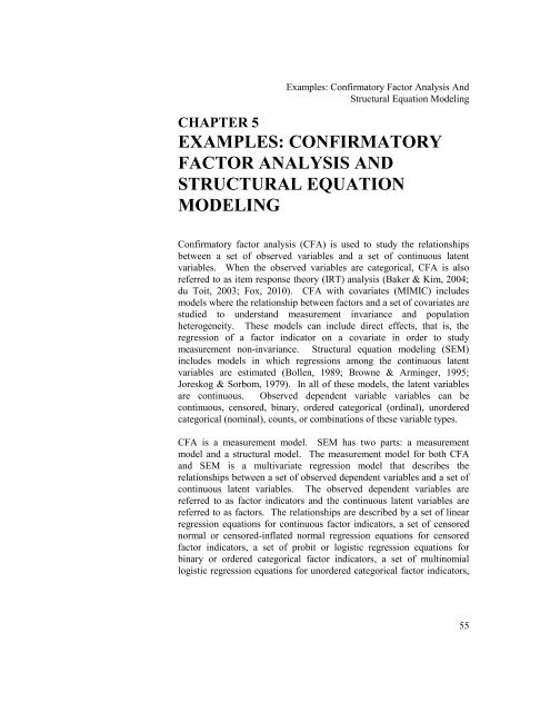
Confirmatory factor analysis (CFA) is used to study the relationships 

between a set of observed variables and a set of continuous latent 

variables. When the observed variables are categorical, CFA is also 

referred to as item response theory (IRT) analysis (Baker & Kim, 2004; 

du Toit, 2003; Fox, 2010). CFA with covariates (MIMIC) includes 

models where the relationship between factors and a set of covariates are 

studied to understand measurement invariance and population 

heterogeneity. These models can include direct effects, that is, the 

regression of a factor indicator on a covariate in order to study 

measurement non-invariance. Structural equation modeling (SEM) 

includes models in which regressions among the continuous latent 

variables are estimated (Bollen, 1989; Browne & Arminger, 1995; 

Joreskog & Sorbom, 1979). In all of these models, the latent variables 

are continuous. Observed dependent variable variables can be 

continuous, censored, binary, ordered categorical (ordinal), unordered 

categorical (nominal), counts, or combinations of these variable types. 

CFA is a measurement model. SEM has two parts: a measurement 

model and a structural model. The measurement model for both CFA 

and SEM is a multivariate regression model that describes the 

relationships between a set of observed dependent variables and a set of 

continuous latent variables. The observed dependent variables are 

referred to as factor indicators and the continuous latent variables are 

referred to as factors. The relationships are described by a set of linear 

regression equations for continuous factor indicators, a set of censored 

normal or censored-inflated normal regression equations for censored 

factor indicators, a set of probit or logistic regression equations for 

binary or ordered categorical factor indicators, a set of multinomial 

logistic regression equations for unordered categorical factor indicators, 

55

CHAPTER 5 

56 

and a set of Poisson or zero-inflated Poisson regression equations for 

count factor indicators. 

The structural model describes three types of relationships in one set of 

multivariate regression equations: the relationships among factors, the 

relationships among observed variables, and the relationships between 

factors and observed variables that are not factor indicators. These 

relationships are described by a set of linear regression equations for the 

factors that are dependent variables and for continuous observed 

dependent variables, a set of censored normal or censored-inflated 

normal regression equations for censored observed dependent variables, 

a set of probit or logistic regression equations for binary or ordered 

categorical observed dependent variables, a set of multinomial logistic 

regression equations for unordered categorical observed dependent 

variables, and a set of Poisson or zero-inflated Poisson regression 

equations for count observed dependent variables. For logistic 

regression, ordered categorical variables are modeled using the 

proportional odds specification. Both maximum likelihood and weighted 

least squares estimators are available. 

All CFA, MIMIC and SEM models can be estimated using the following 

special features: 

� Single or multiple group analysis 

� Missing data 

� Complex survey data 

� Latent variable interactions and non-linear factor analysis using 

maximum likelihood 

� Random slopes 

� Linear and non-linear parameter constraints 

� Indirect effects including specific paths 

� Maximum likelihood estimation for all outcome types 

� Bootstrap standard errors and confidence intervals 

� Wald chi-square test of parameter equalities 

For continuous, censored with weighted least squares estimation, binary, 

and ordered categorical (ordinal) outcomes, multiple group analysis is 

specified by using the GROUPING option of the VARIABLE command 

for individual data or the NGROUPS option of the DATA command for 

summary data. For censored with maximum likelihood estimation, 

unordered categorical (nominal), and count outcomes, multiple group



analysis is specified using the KNOWNCLASS option of the 

VARIABLE command in conjunction with the TYPE=MIXTURE 

option of the ANALYSIS command. The default is to estimate the 

model under missing data theory using all available data. The 

LISTWISE option of the DATA command can be used to delete all 

observations from the analysis that have missing values on one or more 

of the analysis variables. Corrections to the standard errors and chisquare 

test of model fit that take into account stratification, nonindependence 

of observations, and unequal probability of selection are 

obtained by using the TYPE=COMPLEX option of the ANALYSIS 

command in conjunction with the STRATIFICATION, CLUSTER, and 

WEIGHT options of the VARIABLE command. The 

SUBPOPULATION option is used to select observations for an analysis 

when a subpopulation (domain) is analyzed. Latent variable interactions 

are specified by using the | symbol of the MODEL command in 

conjunction with the XWITH option of the MODEL command. Random 

slopes are specified by using the | symbol of the MODEL command in 

conjunction with the ON option of the MODEL command. Linear and 

non-linear parameter constraints are specified by using the MODEL 

CONSTRAINT command. Indirect effects are specified by using the 

MODEL INDIRECT command. Maximum likelihood estimation is 

specified by using the ESTIMATOR option of the ANALYSIS 

command. Bootstrap standard errors are obtained by using the 

BOOTSTRAP option of the ANALYSIS command. Bootstrap 

confidence intervals are obtained by using the BOOTSTRAP option of 

the ANALYSIS command in conjunction with the CINTERVAL option 

of the OUTPUT command. The MODEL TEST command is used to test 

linear restrictions on the parameters in the MODEL and MODEL 

CONSTRAINT commands using the Wald chi-square test. 

Graphical displays of observed data and analysis results can be obtained 

using the PLOT command in conjunction with a post-processing 

graphics module. The PLOT command provides histograms, 

scatterplots, plots of individual observed and estimated values, plots of 

sample and estimated means and proportions/probabilities, and plots of 

item characteristic curves and information curves. These are available 

for the total sample, by group, by class, and adjusted for covariates. The 

PLOT command includes a display showing a set of descriptive statistics 

for each variable. The graphical displays can be edited and exported as a 

DIB, EMF, or JPEG file. In addition, the data for each graphical display 

can be saved in an external file for use by another graphics program. 

57

CHAPTER 5 

58 

Following is the set of CFA examples included in this chapter: 

� 5.1: CFA with continuous factor indicators 

� 5.2: CFA with categorical factor indicators 

� 5.3: CFA with continuous and categorical factor indicators 

� 5.4: CFA with censored and count factor indicators* 

� 5.5: Two-parameter logistic item response theory (IRT) model* 

� 5.6: Second-order factor analysis 

� 5.7: Non-linear CFA* 

� 5.8: CFA with covariates (MIMIC) with continuous factor 

indicators 

� 5.9: Mean structure CFA for continuous factor indicators 

� 5.10: Threshold structure CFA for categorical factor indicators 

Following is the set of SEM examples included in this chapter: 

� 5.11: SEM with continuous factor indicators 

� 5.12: SEM with continuous factor indicators and an indirect effect 

for factors 

� 5.13: SEM with continuous factor indicators and an interaction 

between two factors* 

Following is the set of multiple group examples included in this chapter: 

� 5.14: Multiple group CFA with covariates (MIMIC) with 

continuous factor indicators and no mean structure 


continuous factor indicators and a mean structure 


categorical factor indicators and a threshold structure 


categorical factor indicators and a threshold structure using the 

Theta parameterization 

� 5.18: Two-group twin model for continuous outcomes where factors 

represent the ACE components 

� 5.19: Two-group twin model for categorical outcomes where factors 

represent the ACE components



Following is the set of examples included in this chapter that estimate 

models with parameter constraints: 

� 5.20: CFA with parameter constraints 

� 5.21: Two-group twin model for continuous outcomes using 

parameter constraints 

� 5.22: Two-group twin model for categorical outcomes using 


� 5.23: QTL sibling model for a continuous outcome using parameter 

constraints 

Following is the set of exploratory structural equation modeling (ESEM) 

examples included in this chapter: 

� 5.24: EFA with covariates (MIMIC) with continuous factor 

indicators and direct effects 

� 5.25: SEM with EFA and CFA factors with continuous factor 

indicators 

� 5.26: EFA at two time points with factor loading invariance and 

correlated residuals across time 

� 5.27: Multiple-group EFA with continuous factor indicators 

� 5.28: EFA with residual variances constrained to be greater than 

zero 

� 5.29: Bi-factor EFA using ESEM 

� 5.30: Bi-factor EFA with two items loading on only the general 

factor 

� 5.31: Bayesian bi-factor CFA with two items loading on only the 

general factor and cross-loadings with zero-mean and small-variance 

priors 

� 5.32: Bayesian MIMIC model with cross-loadings and direct effects 

with zero-mean and small-variance priors 

� 5.33: Bayesian multiple group model with approximate 

measurement invariance using zero-mean and small-variance priors 

� Example uses numerical integration in the estimation of the model. 

This can be computationally demanding depending on the size of the 

problem. 

59

CHAPTER 5 

EXAMPLE 5.1: CFA WITH CONTINUOUS FACTOR 

INDICATORS 

60 

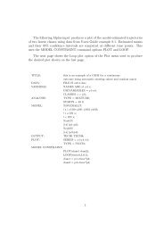
TITLE: this is an example of a CFA with 

continuous factor indicators 

DATA: FILE IS ex5.1.dat; 

VARIABLE: NAMES ARE y1-y6; 

MODEL: f1 BY y1-y3; 

f2 BY y4-y6; 

In this example, the confirmatory factor analysis (CFA) model with 

continuous factor indicators shown in the picture above is estimated. 

The model has two correlated factors that are each measured by three 

continuous factor indicators.





The TITLE command is used to provide a title for the analysis. The title 

is printed in the output just before the Summary of Analysis. 


The DATA command is used to provide information about the data set 

to be analyzed. The FILE option is used to specify the name of the file 

that contains the data to be analyzed, ex5.1.dat. Because the data set is 

in free format, the default, a FORMAT statement is not required. 


The VARIABLE command is used to provide information about the 

variables in the data set to be analyzed. The NAMES option is used to 

assign names to the variables in the data set. The data set in this 

example contains six variables: y1, y2, y3, y4, y5, y6. Note that the 

hyphen can be used as a convenience feature in order to generate a list of 

names. 


f2 BY y4-y6; 

The MODEL command is used to describe the model to be estimated. 

Here the two BY statements specify that f1 is measured by y1, y2, and 

y3, and f2 is measured by y4, y5, and y6. The metric of the factors is set 

automatically by the program by fixing the first factor loading in each 

BY statement to 1. This option can be overridden. The intercepts and 

residual variances of the factor indicators are estimated and the residuals 

are not correlated as the default. The variances of the factors are 

estimated as the default. The factors are correlated as the default 

because they are independent (exogenous) variables. The default 

estimator for this type of analysis is maximum likelihood. The 

ESTIMATOR option of the ANALYSIS command can be used to select 

a different estimator. 

61

CHAPTER 5 

EXAMPLE 5.2: CFA WITH CATEGORICAL FACTOR 

INDICATORS 

62 


categorical factor indicators 


VARIABLE: NAMES ARE u1-u6; 

CATEGORICAL ARE u1-u6; 

MODEL: f1 BY u1-u3; 

f2 BY u4-u6; 

The difference between this example and Example 5.1 is that the factor 

indicators are binary or ordered categorical (ordinal) variables instead of 

continuous variables. The CATEGORICAL option is used to specify 

which dependent variables are treated as binary or ordered categorical 

(ordinal) variables in the model and its estimation. In the example 

above, all six factor indicators are binary or ordered categorical 

variables. The program determines the number of categories for each 

factor indicator. The default estimator for this type of analysis is a 

robust weighted least squares estimator (Muthén, 1984; Muthén, du Toit, 

& Spisic, 1997). With this estimator, probit regressions for the factor 

indicators regressed on the factors are estimated. The ESTIMATOR 

option of the ANALYSIS command can be used to select a different 

estimator. An explanation of the other commands can be found in 

Example 5.1. 

With maximum likelihood estimation, logistic regressions for the factor 

indicators regressed on the factors are estimated using a numerical 

integration algorithm. This is shown in Example 5.5. Note that 

numerical integration becomes increasingly more computationally 

demanding as the number of factors and the sample size increase.

EXAMPLE 5.3: CFA WITH CONTINUOUS AND 

CATEGORICAL FACTOR INDICATORS 




continuous and categorical factor 

indicators 


VARIABLE: NAMES ARE u1-u3 y4-y6; 

CATEGORICAL ARE u1 u2 u3; 


f2 BY y4-y6; 


indicators are a combination of binary or ordered categorical (ordinal) 

and continuous variables instead of all continuous variables. The 

CATEGORICAL option is used to specify which dependent variables 

are treated as binary or ordered categorical (ordinal) variables in the 

model and its estimation. In the example above, the factor indicators u1, 

u2, and u3 are binary or ordered categorical variables whereas the factor 

indicators y4, y5, and y6 are continuous variables. The program 

determines the number of categories for each factor indicator. The 

default estimator for this type of analysis is a robust weighted least 

squares estimator. With this estimator, probit regressions are estimated 

for the categorical factor indicators, and linear regressions are estimated 

for the continuous factor indicators. The ESTIMATOR option of the 

ANALYSIS command can be used to select a different estimator. With 

maximum likelihood estimation, logistic regressions are estimated for 

the categorical dependent variables using a numerical integration 

algorithm. Note that numerical integration becomes increasingly more 

computationally demanding as the number of factors and the sample size 

increase. An explanation of the other commands can be found in 

Example 5.1. 

63

CHAPTER 5 

EXAMPLE 5.4: CFA WITH CENSORED AND COUNT FACTOR 

INDICATORS 

64 

TITLE: this is an example of a CFA with censored 

and count factor indicators 


VARIABLE: NAMES ARE y1-y3 u4-u6; 

CENSORED ARE y1-y3 (a); 

COUNT ARE u4-u6; 


f2 BY u4-u6; 

OUTPUT: TECH1 TECH8; 


indicators are a combination of censored and count variables instead of 

all continuous variables. The CENSORED option is used to specify 

which dependent variables are treated as censored variables in the model 

and its estimation, whether they are censored from above or below, and 

whether a censored or censored-inflated model will be estimated. In the 

example above, y1, y2, and y3 are censored variables. The a in 

parentheses following y1-y3 indicates that y1, y2, and y3 are censored 

from above, that is, have ceiling effects, and that the model is a censored 

regression model. The censoring limit is determined from the data. The 

COUNT option is used to specify which dependent variables are treated 

as count variables in the model and its estimation and whether a Poisson 

or zero-inflated Poisson model will be estimated. In the example above, 

u4, u5, and u6 are count variables. Poisson regressions are estimated for 

the count dependent variables and censored regressions are estimated for 

the censored dependent variables. 

The default estimator for this type of analysis is maximum likelihood 

with robust standard errors using a numerical integration algorithm. 

Note that numerical integration becomes increasingly more 


increase. In this example, two dimensions of integration are used with a 

total of 225 integration points. The ESTIMATOR option of the 

ANALYSIS command can be used to select a different estimator. The 

OUTPUT command is used to request additional output not included as 

the default. The TECH1 option is used to request the arrays containing 

parameter specifications and starting values for all free parameters in the 

model. The TECH8 option is used to request that the optimization



history in estimating the model be printed in the output. TECH8 is 

printed to the screen during the computations as the default. TECH8 

screen printing is useful for determining how long the analysis takes. An 

explanation of the other commands can be found in Example 5.1. 

EXAMPLE 5.5: TWO-PARAMETER LOGISTIC ITEM 

RESPONSE THEORY (IRT) MODEL 

TITLE: this is an example of a two-parameter 

logistic item response theory (IRT) model 


VARIABLE: NAMES ARE u1-u20; 


ANALYSIS: ESTIMATOR = MLR; 

MODEL: f BY u1-u20*; 

f@1; 


PLOT: TYPE = PLOT3; 

In this example, a logistic IRT model is estimated. With binary factor 

indicators, this is referred to as a two-parameter logistic model. With 

ordered categorical (ordinal) factor indicators, this is referred to as 

Samejima’s graded response model (Baker & Kim, 2004; du Toit, 2003). 

A single continuous factor is measured by 20 categorical factor 

indicators. 

The CATEGORICAL option is used to specify which dependent 

variables are treated as binary or ordered categorical (ordinal) variables 

in the model and its estimation. In the example above, the factor 

indicators u1 through u20 are binary or ordered categorical variables. 

The program determines the number of categories for each factor 

indicator. By specifying ESTIMATOR=MLR, a maximum likelihood 

estimator with robust standard errors using a numerical integration 

algorithm will be used. Note that numerical integration becomes 

increasingly more computationally demanding as the number of factors 

and the sample size increase. In this example, one dimension of 

integration is used with 15 integration points. The ESTIMATOR option 

of the ANALYSIS command can be used to select a different estimator. 

In the MODEL command, the BY statement specifies that f is measured 

by u1 through u20. The asterisk (*) frees the first factor loading which 

65

CHAPTER 5 

66 

is fixed at one as the default to define the metric of the factor. Instead 

the metric of the factor is defined by fixing the factor variance at one in 

line with IRT. For one-factor models with no covariates, results are 

presented both in a factor model parameterization and in a conventional 

IRT parameterization. The OUTPUT command is used to request 

additional output not included as the default. The TECH1 option is used 

to request the arrays containing parameter specifications and starting 

values for all free parameters in the model. The TECH8 option is used 

to request that the optimization history in estimating the model be 

printed in the output. TECH8 is printed to the screen during the 

computations as the default. TECH8 screen printing is useful for 

determining how long the analysis takes. The PLOT command is used to 

request graphical displays of observed data and analysis results. These 

graphical displays can be viewed after the analysis is completed using a 

post-processing graphics module. Item characteristic curves and 

information curves are available. When covariates are included in the 

model with direct effects on one or more factor indicators, item 

characteristic curves can be plotted for each value of the covariate to 

show differential item functioning (DIF). An explanation of the other 

commands can be found in Example 5.1. 

EXAMPLE 5.6: SECOND-ORDER FACTOR ANALYSIS 

TITLE: this is an example of a second-order 

factor analysis 




f2 BY y4-y6; 

f3 BY y7-y9; 

f4 BY y10-y12; 

f5 BY f1-f4;



In this example, the second-order factor analysis model shown in the 

figure above is estimated. The factor indicators of the first-order factors 

f1, f2, f3, and f4 are continuous. The first-order factors are indicators of 

the second-order factor f5. 

The first four BY statements specify that f1 is measured by y1, y2, and 

y3; f2 is measured by y4, y5, and y6; f3 is measured by y7, y8, and y9; 

and f4 is measured by y10, y11, and y12. The fifth BY statement 

specifies that the second-order factor f5 is measured by f1, f2, f3, and f4. 

The metrics of the first- and second-order factors are set automatically 

by the program by fixing the first factor loading in each BY statement to 

1. This option can be overridden. The intercepts and residual variances 

of the first-order factor indicators are estimated and the residuals are not 

correlated as the default. The residual variances of the first-order factors 

are estimated as the default. The residuals of the first-order factors are 

not correlated as the default. The variance of the second-order factor is 

estimated as the default. The default estimator for this type of analysis 

is maximum likelihood. The ESTIMATOR option of the ANALYSIS 

command can be used to select a different estimator. An explanation of 

the other commands can be found in Example 5.1. 

67

CHAPTER 5 

EXAMPLE 5.7: NON-LINEAR CFA 

68 

TITLE: this is an example of a non-linear CFA 



ANALYSIS: TYPE = RANDOM; 

ALGORITHM = INTEGRATION; 

MODEL: f BY y1-y5; 

fxf | f XWITH f; 

y1-y5 ON fxf; 


In this example, a non-linear CFA model is estimated (McDonald, 1967). 

The factor indicators are quadratic functions of the factor. The TYPE 

option is used to describe the type of analysis that is to be performed. 

By selecting RANDOM, a model with a random effect will be estimated. 

By specifying ALGORITHM=INTEGRATION, a maximum likelihood 

estimator with robust standard errors using a numerical integration 

algorithm will be used. Note that numerical integration becomes 


and the sample size increase. In this example, one dimension of 

integration is used with 15 integration points. The ESTIMATOR option 

of the ANALYSIS command can be used to select a different estimator. 

The BY statement specifies that f is measured by y1 through y5. This 

specifies the linear part of the quadratic function. The | statement in 

conjunction with the XWITH option of the MODEL command is used to 

define the quadratic factor term. The name on the left-hand side of the | 

symbol names the quadratic factor term. The XWITH statement on the 

right-hand side of the | symbol defines the quadratic factor term fxf. The 

ON statement specifies the quadratic part of the quadratic function. The 

OUTPUT command is used to request additional output not included as 

the default. The TECH1 option is used to request the arrays containing 

parameter specifications and starting values for all free parameters in the 

model. The TECH8 option is used to request that the optimization 

history in estimating the model be printed in the output. TECH8 is 

printed to the screen during the computations as the default. TECH8 

screen printing is useful for determining how long the analysis takes. An 

explanation of the other commands can be found in Example 5.1.



EXAMPLE 5.8: CFA WITH COVARIATES (MIMIC) WITH 

CONTINUOUS FACTOR INDICATORS 


covariates (MIMIC) with continuous factor 

indicators 


VARIABLE: NAMES ARE y1-y6 x1-x3; 


f2 BY y4-y6; 

f1 f2 ON x1-x3; 

In this example, the CFA model with covariates (MIMIC) shown in the 

figure above is estimated. The two factors are regressed on three 

covariates. 

69

CHAPTER 5 

70 

The first BY statement specifies that f1 is measured by y1, y2, and y3. 

The second BY statement specifies that f2 is measured by y4, y5, and y6. 

The metric of the factors is set automatically by the program by fixing 

the first factor loading in each BY statement to 1. This option can be 

overridden. The intercepts and residual variances of the factor 

indicators are estimated and the residuals are not correlated as the 

default. The residual variances of the factors are estimated as the 

default. The residuals of the factors are correlated as the default because 

residuals are correlated for latent variables that do not influence any 

other variable in the model except their own indicators. The ON 

statement describes the linear regressions of f1 and f2 on the covariates 

x1, x2, and x3. The ESTIMATOR option of the ANALYSIS command 

can be used to select a different estimator. An explanation of the other 


EXAMPLE 5.9: MEAN STRUCTURE CFA FOR CONTINUOUS 

FACTOR INDICATORS 

TITLE: this is an example of a mean structure CFA 

for continuous factor indicators 


VARIABLE: NAMES ARE y1a-y1c y2a-y2c; 

MODEL: f1 BY y1a y1b@1 y1c@1; 

f2 BY y2a y2b@1 y2c@1; 

[y1a y1b y1c] (1); 

[y2a y2b y2c] (2);



In this example, the CFA model in which two factors are measured by 

three equivalent tests forms shown in the picture above is estimated. 

The three equivalent test forms are referred to as a, b, and c. 

The first BY statement specifies that f1 is measured by y1a, y1b, and 

y1c. The second BY statement specifies that f2 is measured by y2a, y2b, 

and y2c. The letters a, b, and c are used to represent three equivalent test 

forms, and 1 and 2 represent two different topics. The metric of the 

factors is set automatically by the program by fixing the first factor 

loading in each BY statement to 1. This option can be overridden. The 

second and third factor loadings for both factors are fixed at one using 

the @ option to reflect the hypothesis that the two test forms are 

equivalent. The intercepts and residual variances of the factor indicators 

are estimated and the residuals are not correlated as the default. The 

variances of the factors are estimated as the default. The covariance 

between f1 and f2 is estimated as the default because f1 and f2 are 

independent (exogenous) variables. 

To reflect the hypothesis that the three test forms are equivalent with 

respect to their measurement intercepts, the first bracket statement 

specifies that the intercepts for y1a, y1b, and y1c are equal and the 

71

CHAPTER 5 

72 

second bracket statement specifies that the intercepts for y2a, y2b, and 

y2c are equal. Equalities are designated by a number in parentheses. All 

parameters in a statement followed by the same number in parentheses 

are held equal. The means of the two factors are fixed at zero as the 

default. The default estimator for this type of analysis is maximum 

likelihood. The ESTIMATOR option of the ANALYSIS command can 

be used to select a different estimator. An explanation of the other 


EXAMPLE 5.10: THRESHOLD STRUCTURE CFA FOR 

CATEGORICAL FACTOR INDICATORS 

TITLE: this is an example of a threshold 

structure CFA for categorical factor 

indicators 


VARIABLE: NAMES ARE u1a-u1c u2a-u2c; 

CATEGORICAL ARE u1a-u1c u2a-u2c; 

MODEL: f1 BY u1a u1b@1 u1c@1; 

f2 BY u2a u2b@1 u2c@1; 

[u1a$1 u1b$1 u1c$1] (1); 

[u2a$1 u2b$1 u2c$1] (2); 



continuous variables. The CATEGORICAL option is used to specify 

which dependent variables are treated as binary or ordered categorical 

(ordinal) variables in the model and its estimation. In the example 

above, all six factor indicators are binary or ordered categorical 

variables. The program determines the number of categories for each 

factor indicator. In this example, it is assumed that the factor indicators 

are binary variables with one threshold each. 

For binary and ordered categorical factor indicators, thresholds are 

modeled rather than intercepts or means. The number of thresholds for a 

categorical variable is equal to the number of categories minus one. In 

the example above, the categorical variables are binary so they have one 

threshold. Thresholds are referred to by adding to the variable name a $ 

followed by a number. The thresholds of the factor indicators are 

referred to as u1a$1, u1b$1, u1c$1, u2a$1, u2b$1, and u2c$1. 

Thresholds are referred to in square brackets. To reflect the hypothesis



that the three test forms are equivalent with respect to their measurement 

thresholds, the (1) after the first bracket statement specifies that the 

thresholds for u1a, u1b, and u1c are constrained to be equal and the (2) 

after the second bracket statement specifies that the thresholds for u2a, 

u2b, and u2c are constrained to be equal. The default estimator for this 

type of analysis is a robust weighted least squares estimator. The 


a different estimator. With maximum likelihood, logistic regressions are 

estimated using a numerical integration algorithm. Note that numerical 

integration becomes increasingly more computationally demanding as 

the number of factors and the sample size increase. An explanation of 

the other commands can be found in Examples 5.1 and 5.9. 

EXAMPLE 5.11: SEM WITH CONTINUOUS FACTOR 

INDICATORS 

TITLE: this is an example of a SEM with 





f2 BY y4-y6; 

f3 BY y7-y9; 

f4 BY y10-y12; 

f4 ON f3; 

f3 ON f1 f2; 

73

CHAPTER 5 

74 

In this example, the SEM model with four continuous latent variables 

shown in the picture above is estimated. The factor indicators are 

continuous variables. 

The first BY statement specifies that f1 is measured by y1, y2 and y3. 

The second BY statement specifies that f2 is measured by y4, y5, and y6. 

The third BY statement specifies that f3 is measured by y7, y8, and y9. 

The fourth BY statement specifies that f4 is measured by y10, y11, and 

y12. The metric of the factors is set automatically by the program by 

fixing the first factor loading in each BY statement to 1. This option can 

be overridden. The intercepts and residual variances of the factor 


default. The variances of the factors are estimated as the default. The 

covariance between f1 and f2 is estimated as the default because f1 and 

f2 are independent (exogenous) variables. The other factor covariances 

are not estimated as the default. 

The first ON statement describes the linear regression of f4 on f3. The 

second ON statement describes the linear regression of f3 on f1 and f2. 

The default estimator for this type of analysis is maximum likelihood. 

The ESTIMATOR option of the ANALYSIS command can be used to 

select a different estimator. An explanation of the other commands can 

be found in Example 5.1.




INDICATORS AND AN INDIRECT EFFECT FOR FACTORS 


continuous factor indicators and an 

indirect effect for factors 




f2 BY y4-y6; 

f3 BY y7-y9; 

f4 BY y10-y12; 

f4 ON f3; 

f3 ON f1 f2; 

MODEL INDIRECT: 

f4 IND f3 f1; 

The difference between this example and Example 5.11 is that an 

indirect effect is estimated. Indirect effects and their standard errors can 

be requested using the MODEL INDIRECT command. Total indirect, 

specific indirect, and total effects are specified by using the IND and 

VIA statements. Total effects include all indirect effects and the direct 

effect. The IND statement is used to request a specific indirect effect or 

set of indirect effects. The VIA statement is used to request a set of 

indirect effects that include specific mediators. 

In the IND statement above, the variable on the left-hand side of IND is 

the dependent variable. The last variable on the right-hand side of IND 

is the independent variable. Other variables on the right-hand side of 

IND are mediating variables. The IND statement requests the specific 

indirect effect from f1 to f3 to f4. The default estimator for this type of 

analysis is maximum likelihood. The ESTIMATOR option of the 

ANALYSIS command can be used to select a different estimator. An 

explanation of the other commands can be found in Examples 5.1 and 

5.11. 

75

CHAPTER 5 


INDICATORS AND AN INTERACTION BETWEEN TWO 

LATENT VARIABLES 

76 


continuous factor indicators and an 

interaction between two latent variables 



ANALYSIS: TYPE = RANDOM; 

ALGORITHM = INTEGRATION; 


f2 BY y4-y6; 

f3 BY y7-y9; 

f4 BY y10-y12; 

f4 ON f3; 

f3 ON f1 f2; 

f1xf2 | f1 XWITH f2; 

f3 ON f1xf2; 


The difference between this example and Example 5.11 is that an 

interaction between two latent variables is included in the model. The



interaction is shown in the picture above as a filled circle. The model is 

estimated using maximum likelihood (Klein & Moosbrugger, 2000). 

The TYPE option is used to describe the type of analysis that is to be 

performed. By selecting RANDOM, a model with a random effect will 

be estimated. By specifying ALGORITHM=INTEGRATION, a 

maximum likelihood estimator with robust standard errors using a 

numerical integration algorithm will be used. Note that numerical 

integration becomes increasingly more computationally demanding as 

the number of factors and the sample size increase. In this example, two 

dimensions of integration are used with a total of 225 integration points. 


select a different estimator. 

Latent variable interactions are specified by using the | statement in 

conjunction with the XWITH option of the MODEL command. The 

name on the left-hand side of the | symbol names the latent variable 

interaction. The XWITH statement on the right-hand side of the | 

symbol defines the latent variable interaction. The latent variable f1xf2 

is the interaction between f1 and f2. The last ON statement uses the 

latent variable interaction as an independent variable. The OUTPUT 

command is used to request additional output not included as the default. 

The TECH1 option is used to request the arrays containing parameter 

specifications and starting values for all free parameters in the model. 

The TECH8 option is used to request that the optimization history in 

estimating the model be printed in the output. TECH8 is printed to the 

screen during the computations as the default. TECH8 screen printing is 

useful for determining how long the analysis takes. An explanation of 

the other commands can be found in Examples 5.1 and 5.11. 

77

CHAPTER 5 

EXAMPLE 5.14: MULTIPLE GROUP CFA WITH 

COVARIATES (MIMIC) WITH CONTINUOUS FACTOR 

INDICATORS AND NO MEAN STRUCTURE 

78 

TITLE: this is an example of a multiple group CFA 

with covariates (MIMIC) with continuous 

factor indicators and no mean structure 


VARIABLE: NAMES ARE y1-y6 x1-x3 g; 

GROUPING IS g (1 = male 2 = female); 

ANALYSIS: MODEL = NOMEANSTRUCTURE; 

INFORMATION = EXPECTED; 


f2 BY y4-y6; 

f1 f2 ON x1-x3; 

MODEL female: 

f1 BY y3; 

The difference between this example and Example 5.8 is that this is a 

multiple group rather than a single group analysis. The GROUPING 

option is used to identify the variable in the data set that contains 

information on group membership when the data for all groups are 

stored in a single data set. The information in parentheses after the 

grouping variable name assigns labels to the values of the grouping 

variable found in the data set. In the example above, observations with g 

equal to 1 are assigned the label male, and individuals with g equal to 2 

are assigned the label female. These labels are used in conjunction with 

the MODEL command to specify model statements specific to each 

group. 

The NOMEANSTRUCTURE setting for the MODEL option of the 

ANALYSIS command is used with TYPE=GENERAL to specify that 

means, intercepts, and thresholds are not included in the analysis model. 

As a result, a covariance structure model is estimated. The 

INFORMATION option is used to select the estimator of the information 

matrix to be used in computing standard errors when the ML or MLR 

estimators are used for analysis. The default is the observed information 

matrix. In this example, the expected information matrix is used in line 

with conventional covariance structure analysis.



In multiple group analysis, two variations of the MODEL command are 

used. They are MODEL and MODEL followed by a label. MODEL 

describes the overall model to be estimated for each group. The factor 

loading measurement parameters are held equal across groups as the 

default to specify measurement invariance. MODEL followed by a label 

describes differences between the overall model and the model for the 

group designated by the label. In the group-specific MODEL command 

for females, the factor loading for variable y3 and factor f1 is specified 

to be free and not equal to the same factor loading for males. The 

default estimator for this type of analysis is maximum likelihood. The 


a different estimator. An explanation of the other commands can be 

found in Examples 5.1 and 5.8. 


COVARIATES (MIMIC) WITH CONTINUOUS FACTOR 

INDICATORS AND A MEAN STRUCTURE 


with covariates (MIMIC) with continuous 

factor indicators and a mean structure 


VARIABLE: NAMES ARE y1-y6 x1-x3 g; 



f2 BY y4-y6; 

f1 f2 ON x1-x3; 

MODEL female: 

f1 BY y3; 

[y3]; 

The difference between this example and Example 5.14 is that means are 

included in the model. In multiple group analysis, when a model 

includes a mean structure, both the intercepts and factor loadings of the 

continuous factor indicators are held equal across groups as the default 

to specify measurement invariance. The intercepts of the factors are 

fixed at zero in the first group and are free to be estimated in the other 

groups as the default. The group-specific MODEL command for 

females specifies that the intercept of y3 for females is free and not 

equal to the intercept for males. Intercepts are referred to by using 

square brackets. The default estimator for this type of analysis is 

79

CHAPTER 5 

80 

maximum likelihood. The ESTIMATOR option of the ANALYSIS 


the other commands can be found in Examples 5.1, 5.8, and 5.14. 


COVARIATES (MIMIC) WITH CATEGORICAL FACTOR 

INDICATORS AND A THRESHOLD STRUCTURE 


with covariates (MIMIC) with categorical 

factor indicators and a threshold 

structure 


VARIABLE: NAMES ARE u1-u6 x1-x3 g; 




f2 BY u4-u6; 

f1 f2 ON x1-x3; 

MODEL female: 

f1 BY u3; 

[u3$1]; 

{u3@1}; 



continuous variables. For multiple-group CFA with categorical factor 

indicators, see Muthén and Christoffersson (1981) and Muthén and 

Asparouhov (2002). 



in the model and its estimation. In the example above, all six factor 

indicators are binary or ordered categorical variables. The program 

determines the number of categories for each factor indicator. 

For binary and ordered categorical factor indicators, thresholds are 

modeled rather than intercepts or means. The number of thresholds for a 


the above example, u3 is a binary variable with two categories. 

Thresholds are referred to by adding to the variable name a $ followed 

by a number. The threshold for u3 is u3$1. Thresholds are referred to in



square brackets. When a model includes a mean structure, the 

thresholds of the factor indicators are held equal across groups as the 

default to specify measurement invariance. In the group-specific 

MODEL command for females, the threshold and factor loading of u3 

for females are specified to be free and not equal to the threshold and 

factor loading for males. 

Because the factor indicators are categorical, scale factors are required 

for multiple group analysis when the default Delta parameterization is 

used. Scale factors are referred to using curly brackets ({}). By default, 

scale factors are fixed at one in the first group and are free to be 

estimated in the other groups. When a threshold and a factor loading for 

a categorical factor indicator are free across groups, the scale factor for 

that variable must be fixed at one in all groups for identification 

purposes. Therefore, the scale factor for u3 is fixed at one for females. 

The default estimator for this type of analysis is a robust weighted least 

squares estimator. The ESTIMATOR option of the ANALYSIS 

command can be used to select a different estimator. With maximum 

likelihood, logistic regressions are estimated using a numerical 

integration algorithm. Note that numerical integration becomes 


and the sample size increase. An explanation of the other commands can 

be found in Examples 5.1, 5.8, 5.14, and 5.15. 

81

CHAPTER 5 


COVARIATES (MIMIC) WITH CATEGORICAL FACTOR 

INDICATORS AND A THRESHOLD STRUCTURE USING THE 

THETA PARAMETERIZATION 

82 


with covariates (MIMIC) with categorical 

factor indicators and a threshold 

structure using the Theta parameterization 


VARIABLE: NAMES ARE u1-u6 x1-x3 g; 



ANALYSIS: PARAMETERIZATION = THETA; 


f2 BY u4-u6; 

f1 f2 ON x1-x3; 

MODEL female: 

f1 BY u3; 

[u3$1]; 

u3@1; 

The difference between this example and Example 5.16 is that the Theta 

parameterization is used instead of the Delta parameterization. In the 

Delta parameterization, scale factors are allowed to be parameters in the 

model, but residual variances for latent response variables of observed 

categorical dependent variables are not. In the alternative Theta 

parameterization, residual variances for latent response variables are 

allowed to be parameters in the model but scale factors are not. The 

Theta parameterization is selected by specifying 

PARAMETERIZATION=THETA in the ANALYSIS command. 

When the Theta parameterization is used, the residual variances for the 

latent response variables of the observed categorical dependent variables 

are fixed at one in the first group and are free to be estimated in the other 

groups as the default. When a threshold and a factor loading for a 

categorical factor indicator are free across groups, the residual variance 

for the variable must be fixed at one in these groups for identification 

purposes. In the group-specific MODEL command for females, the 

residual variance for u3 is fixed at one. An explanation of the other 

commands can be found in Examples 5.1, 5.8, 5.14, 5.15, and 5.16.



EXAMPLE 5.18: TWO-GROUP TWIN MODEL FOR 

CONTINUOUS OUTCOMES WHERE FACTORS REPRESENT 

THE ACE COMPONENTS 

TITLE: this is an example of a two-group twin 

model for continuous outcomes where 

factors represent the ACE components 

DATA: FILE = ex5.18.dat; 

VARIABLE: NAMES = y1 y2 g; 

GROUPING = g (1 = mz 2 = dz); 

ANALYSIS: MODEL = NOCOVARIANCES; 

MODEL: [y1-y2] (1); 

y1-y2@0; 

a1 BY y1* (2); 

a2 BY y2* (2); 

c1 BY y1* (3); 

c2 BY y2* (3); 

e1 BY y1* (4); 

e2 BY y2* (4); 

a1-e2@1; 

[a1-e2@0]; 

a1 WITH a2@1; 

c1 WITH c2@1; 

MODEL dz: a1 WITH a2@.5; 

In this example, the univariate twin model shown in the picture above is 

estimated. This is a two-group twin model for a continuous outcome 

where factors represent the ACE components (Neale & Cardon, 1992). 

83

CHAPTER 5 

84 

The variables y1 and y2 represent a univariate outcome for each member 

of the twin pair. The A factors represent the additive genetic 

components which correlate 1.0 for monozygotic twin pairs and 0.5 for 

dizygotic twin pairs. The C factors represent common environmental 

effects which correlate 1.0 for all twin pairs. The E factors represent 

uncorrelated environmental effects. A simpler alternative way of 

specifying this model is shown in Example 5.21 where parameter 

constraints are used instead of the A, C, and E factors. 

Exogenous factors are correlated as the default. By specifying 

MODEL=NOCOVARIANCES in the ANALYSIS command, all 

covariances in the model are fixed at zero. The WITH option of the 

MODEL command can be used to override the default for selected 

covariances as shown in the three WITH statements. In the MODEL 

command, the (1) following the first bracket statement specifies that the 

intercepts of y1 and y2 are held equal across twins. The second 

statement fixes the residual variances of y1 and y2 to zero. The residual 

variances of y1 and y2 are instead captured by the loadings of the E 

factors. The six BY statements are used to define the six factors. The 

asterisk (*) is used to free the factor loadings because the default is that 

the factor loading for the first factor indicator is fixed at one. The 

loadings for the A, C, and E factors are held equal across twins by 

placing (2) following the two BY statements for the A factors, (3) 

following the two BY statements for the C factors, and (4) following the 

two BY statements for the E factors. In the next two statements, the A, 

C, and E factor variances are fixed at one and the A, C, and E factor 

means are fixed at zero. Because the factor means are fixed at zero, the 

intercepts of y1 and y2 are their means. 

The WITH statement for the A factors is used to fix the covariance 

(correlation) between the A factors to 1.0 for monozygotic twin pairs. 

The group-specific MODEL command is used to fix the covariance 

between the A factors to 0.5 for the dizygotic twin pairs. The WITH 

statement for the C factors is used to fix the covariance between the C 

factors to 1. The default estimator for this type of analysis is maximum 



commands can be found in Examples 5.1 and 5.14.




CATEGORICAL OUTCOMES WHERE FACTORS 

REPRESENT THE ACE COMPONENTS 


model for categorical outcomes where 

factors represent the ACE components 


VARIABLE: NAMES = u1 u2 g; 

CATEGORICAL = u1-u2; 

GROUPING = g (1 = mz 2 = dz); 

ANALYSIS: MODEL = NOCOVARIANCES; 

MODEL: [u1$1-u2$1] (1); 

a1 BY u1* (2); 

a2 BY u2* (2); 

c1 BY u1* (3); 

c2 BY u2* (3); 

a1-c2@1; 

[a1-c2@0]; 

a1 WITH a2@1; 

c1 WITH c2@1; 

MODEL dz: a1 WITH a2@.5; 

{u1-u2@1}; 

The difference between this example and Example 5.18 is that the 

outcomes are binary or ordered categorical instead of continuous 

variables. Because of this, the outcomes have no freely estimated 

residual variances and therefore the E factors are not part of the model. 

With categorical outcomes, the twin model is formulated for normallydistributed 

latent response variables underlying the categorical outcomes 

which are also called liabilities. This model is referred to as the 

threshold model for liabilities (Neale & Cardon, 1992). More complex 

examples of such models are given in Prescott (2004). A simpler 

alternative way of specifying this model is shown in Example 5.22 

where parameter constraints are used instead of the A and C factors. 



in the model and its estimation. In the example above, u1 and u2 are 

binary or ordered categorical variables. The program determines the 

number of categories for each variable. 

85

CHAPTER 5 

86 

For binary and ordered categorical outcomes, thresholds are modeled 

rather than intercepts or means. The number of thresholds for a 


the example above, the categorical variables are binary so they have one 

threshold. Thresholds are referred to by adding to the variable name a $ 

followed by a number. The thresholds of u1 and u2 are referred to as 

u1$1 and u2$1. Thresholds are referred to in square brackets. The (1) 

after the first bracket statement specifies that the thresholds for u1$1 and 

u2$1 are constrained to be equal. 

Because the outcomes are categorical, scale factors are required for 

multiple group analysis when the default Delta parameterization is used. 

Scale factors are referred to using curly brackets ({}). By default, scale 

factors are fixed at one in the first group and are free to be estimated in 

the other groups. In this model where the variance contributions from 

the A and C factors are assumed equal across the two groups, the scale 

factors are fixed at one in both groups to represent the equality of 

variance for latent response variables underlying u1 and u2. The 

statement in curly brackets in the group-specific MODEL command 

specifies that the scale factors are fixed at one. The variance 

contribution from the E factor is a remainder obtained by subtracting the 

variance contributions of the A and C factors from the unit variance of 

the latent response variables underlying u1 and u2. These are obtained 

as part of the STANDARDIZED option of the OUTPUT command. 




likelihood and categorical factor indicators, numerical integration is 

required. Note that numerical integration becomes increasingly more 


increase. An explanation of the other commands can be found in 

Examples 5.1, 5.14, and 5.18.



EXAMPLE 5.20: CFA WITH PARAMETER CONSTRAINTS 

TITLE: this is an example of a CFA with parameter 

constraints 


VARIABLE: NAMES = y1-y6; 

MODEL: f1 BY y1 

y2-y3(lam2-lam3); 

f2 BY y4 

y5-y6(lam5-lam6); 

f1 (vf1); 

f2 (vf2); 

y1-y3 (ve1-ve3); 

y4-y6 (ve4-ve6); 

MODEL CONSTRAINT: 

NEW(rel2 rel5 stan3 stan6); 

rel2 = lam2**2*vf1/(lam2**2*vf1 + ve2); 

rel5 = lam5**2*vf2/(lam5**2*vf2 + ve5); 

rel5 = rel2; 

stan3 = lam3*SQRT(vf1)/SQRT(lam3**2*vf1 + 

ve3); 

stan6 = lam6*SQRT(vf2)/SQRT(lam6**2*vf2 + 

ve6); 

0 = stan6 - stan3; 

ve2 > ve5; 

ve4 > 0; 

OUTPUT: STANDARDIZED; 

In this example, parameter constraints are used to estimate reliabilities, 

estimate standardized coefficients, constrain functions of parameters to 

be equal, and constrain parameters to be greater than a value. This 

example uses the model from Example 5.1. 

The MODEL CONSTRAINT command specifies parameter constraints 

using labels defined for parameters in the MODEL command, labels 

defined for parameters not in the MODEL command using the NEW 

option of the MODEL CONSTRAINT command, and names of observed 

variables that are identified using the CONSTRAINT option of the 

VARIABLE command. This example illustrates constraints using labels 

defined for parameters in the MODEL command and labels defined 

using the NEW option. The NEW option is used to assign labels and 

starting values to parameters not in the analysis model. Parameters in 

the analysis model are given labels by placing a name in parentheses 

after the parameter in the MODEL command. 

87

CHAPTER 5 

88 

In the MODEL command, labels are defined for twelve parameters. The 

list function can be used when assigning labels to a list of parameters. 

The labels lam2, lam3, lam5, and lam6 are assigned to the factor 

loadings for y2, y3, y5, and y6. The labels vf1 and vf2 are assigned to 

the factor variances for f1 and f2. The labels ve1, ve2, ve3, ve4, ve5, 

and ve6 are assigned to the residual variances of y1, y2, y3, y4, y5, and 

y6. 

In the MODEL CONSTRAINT command, the NEW option is used to 

assign labels to four parameters that are not in the analysis model: rel2, 

rel5, stan3, and stan6. The parameters rel2 and rel6 estimate the 

reliability of y2 and y6 where reliability is defined as variance explained 

divided by total variance. The parameters stan3 and stan6 estimate the 

standardized coefficients for y3 and y6 using conventional 

standardization formulas. In the statement that begins 0=, two 

parameters are held equal to each other by defining their difference as 

zero. In the last two statements, the residual variance of y2 is 

constrained to be greater than the residual variance of y5, and the 

residual variance of y4 is constrained to be greater than zero. The 

STANDARDIZED option of the OUTPUT command is requested to 

illustrate that the R-square values found in the output are the same as the 

estimated reliabilities, and the standardized values found in the output 

are the same as the estimated standardized values. Standard errors for 

parameters named using the NEW option are given. The default 

estimator for this type of analysis is maximum likelihood. The 


a different estimator. An explanation of the other commands can be 

found in Example 5.1.




CONTINUOUS OUTCOMES USING PARAMETER 

CONSTRAINTS 


model for continuous outcomes using 



VARIABLE: NAMES = y1 y2 g; 

GROUPING = g(1 = mz 2 = dz); 

MODEL: [y1-y2] (1); 

y1-y2 (var); 

y1 WITH y2 (covmz); 

MODEL dz: y1 WITH y2 (covdz); 


NEW(a c e h); 

var = a**2 + c**2 + e**2; 

covmz = a**2 + c**2; 

covdz = 0.5*a**2 + c**2; 

h = a**2/(a**2 + c**2 + e**2); 

In this example, the model shown in the picture above is estimated using 

parameter constraints. The model estimated is the same as the model in 

Example 5.18. 

In the MODEL command, labels are defined for three parameters. The 

label var is assigned to the variances of y1 and y2. Because they are 

given the same label, these parameters are held equal. In the overall 

MODEL command, the label covmz is assigned to the covariance 

between y1 and y2 for the monozygotic twins. In the group-specific 

MODEL command, the label covdz is assigned to the covariance 

between y1 and y2 for the dizygotic twins. 


assign labels to four parameters that are not in the analysis model: a, c, 

89

CHAPTER 5 

90 

e, and h. The three parameters a, c, and e are used to decompose the 

variances and covariances of y1 and y2 into genetic and environmental 

components. The parameter h does not impose restrictions on the model 

parameters but is used to compute the heritability estimate and its 

standard error. The default estimator for this type of analysis is 



the other commands can be found in Examples 5.1, 5.14, 5.18, and 5.20. 


CATEGORICAL OUTCOMES USING PARAMETER 

CONSTRAINTS 


model for categorical outcomes using 



VARIABLE: NAMES = u1 u2 g; 

GROUPING = g(1 = mz 2 = dz); 

CATEGORICAL = u1 u2; 

MODEL: [u1$1-u2$1](1); 

u1 WITH u2(covmz); 

MODEL dz: u1 WITH u2(covdz); 


NEW(a c e h); 

covmz = a**2 + c**2; 

covdz = 0.5*a**2 + c**2; 

e = 1 - (a**2 + c**2); 

h = a**2/1; 

The difference between this example and Example 5.21 is that the 

outcomes are binary or ordered categorical instead of continuous 

variables. Because of this, the outcomes have no freely estimated 

residual variances. The ACE variance and covariance restrictions are 

placed on normally-distributed latent response variables underlying the 

categorical outcomes which are also called liabilities. This model is 

referred to as the threshold model for liabilities (Neale & Cardon, 1992). 

The model estimated is the same as the model in Example 5.19. 

The variance contribution from the E factor is not a freely estimated 

parameter with categorical outcomes. It is a remainder obtained by 

subtracting the variance contributions of the A and C factors from the



unit variance of the latent response variables underlying u1 and u2 as 

shown in the MODEL CONSTRAINT command. The denominator for 

the heritability estimate is one with categorical outcomes because the 

latent response variables have unit variances. 




likelihood, logistic or probit regressions are estimated using a numerical 

integration algorithm. Note that numerical integration becomes 


and the sample size increase. An explanation of the other commands can 

be found in Examples 5.1, 5.14, 5.19 and 5.21. 

EXAMPLE 5.23: QTL SIBLING MODEL FOR A CONTINUOUS 

OUTCOME USING PARAMETER CONSTRAINTS 

TITLE: this is an example of a QTL sibling model 

for a continuous outcome using parameter 

constraints 


VARIABLE: NAMES = y1 y2 pihat; 

USEVARIABLES = y1 y2; 

CONSTRAINT = pihat; 

MODEL: [y1-y2] (1); 

y1-y2 (var); 

y1 WITH y2 (cov); 


NEW(a e q); 

var = a**2 + e**2 + q**2; 

cov = 0.5*a**2 + pihat*q**2; 

91

CHAPTER 5 

92 

In this example, the model shown in the picture above is estimated. This 

is a QTL model for two siblings (Marlow et al. 2003; Posthuma et al. 

2004) for continuous outcomes where parameter constraints are used to 

represent the A, E, and Q components. The A component represents the 

additive genetic effects which correlate 0.5 for siblings. The E 

component represents uncorrelated environmental effects. The Q 

component represents a quantitative trait locus (QTL). The observed 

variable pihat contains the estimated proportion alleles shared identityby-descent 

(IBD) by the siblings and moderates the effect of the Q 

component on the covariance between the outcomes. 

The CONSTRAINT option in the VARIABLE command is used to 

identify the variables that can be used in the MODEL CONSTRAINT 

command. These can be not only variables used in the MODEL 

command but also other variables. In this example, the variable pihat is 

used in the MODEL CONSTRAINT command although it is not used in 

the MODEL command. 

In the MODEL command, the (1) following the first bracket statement 

specifies that the intercepts of y1 and y2 are held equal across the two 

siblings. In addition, labels are defined for two parameters. The label 

var is assigned to the variances of y1 and y2. Because they are given the 

same label, these parameters are held equal. The label cov is assigned to 

the covariance between y1 and y2. 


assign labels to three parameters that are not in the analysis model: a, e, 

and q. The three parameters a, e, and q and the variable pihat are used to 

decompose the variances and covariances of y1 and y2 into genetic, 

environmental, and QTL components. The default estimator for this 

type of analysis is maximum likelihood. The ESTIMATOR option of 

the ANALYSIS command can be used to select a different estimator. 

An explanation of the other commands can be found in Examples 5.1 

and 5.20.



EXAMPLE 5.24: EFA WITH COVARIATES (MIMIC) WITH 

CONTINUOUS FACTOR INDICATORS AND DIRECT 

EFFECTS 

TITLE: this is an example of an EFA with 

covariates (MIMIC) with continuous factor 

indicators and direct effects 


VARIABLE: NAMES ARE y1-y8 x1 x2; 

MODEL: f1-f2 BY y1-y8(*1); 

f1-f2 ON x1-x2; 

y1 ON x1; 

y8 ON x2; 

OUTPUT: TECH1; 

In this example, the EFA with covariates (MIMIC) with continuous 

factor indicators and direct effects shown in the picture above is 

93

CHAPTER 5 

94 

estimated. This is an exploratory structural equation model (ESEM; 

Asparouhov & Muthén, 2009a). The factors f1 and f2 are EFA factors 

which have the same factor indicators. Unlike CFA, no factor loadings 

are fixed at zero. Instead, the four restrictions on the factor loadings, 

factor variances, and factor covariances necessary for identification are 

imposed by rotating the factor loading matrix and fixing the factor 

residual variances at one. 

In the MODEL command, the BY statement specifies that the factors f1 

and f2 are measured by the continuous factor indicators y1 through y8. 

The label 1 following an asterisk (*) in parentheses following the BY 

statement is used to indicate that f1 and f2 are a set of EFA factors. 

When no rotation is specified using the ROTATION option of the 

ANALYSIS command, the default oblique GEOMIN rotation is used. 

The intercepts and residual variances of the factor indicators are 

estimated and the residuals are not correlated as the default. The 

residual variances of the factors are fixed at one as the default. The 

residuals of the factors are correlated under the default oblique 

GEOMIN rotation. The first ON statement describes the linear 

regressions of f1 and f2 on the covariates x1 and x2. The second and 

third ON statements describe the linear regressions of y1 on x1 and y8 

on x2. These regressions represent direct effects used to test for 

measurement non-invariance. 

The default estimator for this type of analysis is maximum likelihood. 


select a different estimator. An explanation of the other commands can 

be found in Example 5.1.



EXAMPLE 5.25: SEM WITH EFA AND CFA FACTORS WITH 


TITLE: this is an example of a SEM with EFA and 

CFA factors with continuous factor 

indicators 



MODEL: f1-f2 BY y1-y6 (*1); 

f3 BY y7-y9; 

f4 BY y10-y12; 

f3 ON f1-f2; 

f4 ON f3; 

In this example, the SEM with EFA and CFA factors with continuous 

factor indicators shown in the picture above is estimated. This is an 

exploratory structural equation model (ESEM; Asparouhov & Muthén, 

2009a). The factors f1 and f2 are EFA factors which have the same 

factor indicators. Unlike CFA, no factor loadings are fixed at zero. 

Instead, the four restrictions on the factor loadings, factor variances, and 

factor covariances necessary for identification are imposed by rotating 

95

CHAPTER 5 

96 

the factor loading matrix and fixing the factor variances at one. The 

factors f3 and f4 are CFA factors. 

In the MODEL command, the first BY statement specifies that the 

factors f1 and f2 are measured by the continuous factor indicators y1 

through y6. The label 1 following an asterisk (*) in parentheses 

following the BY statement is used to indicate that f1 and f2 are a set of 

EFA factors. When no rotation is specified using the ROTATION 

option of the ANALYSIS command, the default oblique GEOMIN 

rotation is used. For EFA factors, the intercepts and residual variances 

of the factor indicators are estimated and the residuals are not correlated 

as the default. The variances of the factors are fixed at one as the 

default. The factors are correlated under the default oblique GEOMIN 

rotation. The second BY statement specifies that f3 is measured by y7, 

y8, and y9. The third BY statement specifies that f4 is measured by y10, 

y11, and y12. The metric of the factors is set automatically by the 

program by fixing the first factor loading in each BY statement to 1. 

This option can be overridden. The intercepts and residual variances of 

the factor indicators are estimated and the residual are not correlated as 

the default. The residual variances of the factors are estimated as the 

default. 

The first ON statement describes the linear regression of f3 on the set of 

EFA factors f1 and f2. The second ON statement describes the linear 

regression of f4 on f3. The default estimator for this type of analysis is 



the other commands can be found in Example 5.1.



EXAMPLE 5.26: EFA AT TWO TIME POINTS WITH FACTOR 

LOADING INVARIANCE AND CORRELATED RESIDUALS 

ACROSS TIME 

TITLE: this is an example of an EFA at two time 

points with factor loading invariance and 

correlated residuals across time 



MODEL: f1-f2 BY y1-y6 (*t1 1); 

f3-f4 BY y7-y12 (*t2 1); 

y1-y6 PWITH y7-y12; 

OUTPUT: TECH1 STANDARDIZED; 

In this example, the EFA at two time points with factor loading 

invariance and correlated residuals across time shown in the picture 

above is estimated. This is an exploratory structural equation model 

(ESEM; Asparouhov & Muthén, 2009a). The factor indicators y1 

through y6 and y7 through y12 are the same variables measured at two 

time points. The factors f1 and f2 are one set of EFA factors which have 

the same factor indicators and the factors f3 and f4 are a second set of 

EFA factors which have the same factor indicators. Unlike CFA, no 

factor loadings are fixed at zero in either set. Instead, for each set, the 

four restrictions on the factor loadings, factor variances, and factor 

covariances necessary for identification are imposed by rotating the 

factor loading matrix and fixing the factor variances at one at the first 

time point. For the other time point, factor variances are free to be 

97

CHAPTER 5 

98 

estimated as the default when factor loadings are constrained to be equal 

across time. 


factors f1 and f2 are measured by the continuous factor indicators y1 

through y6. The label t1 following an asterisk (*) in parentheses 

following the BY statement is used to indicate that f1 and f2 are a set of 

EFA factors. The second BY statement specifies that the factors f3 and 

f4 are measured by the continuous factor indicators y7 through y12. The 

label t2 following an asterisk (*) in parentheses following the BY 

statement is used to indicate that f3 and f4 are a set of EFA factors. The 

number 1 following the labels t1 and t2 specifies that the factor loadings 

matrices for the two sets of EFA factors are constrained to be equal. 



For EFA factors, the intercepts and residual variances of the factor 


default. The intercepts are not held equal across time as the default. 

The means of the factors are fixed at zero at both time points and the 

variances of the factors are fixed at one as the default. In this example 

because the factor loadings are constrained to be equal across time, the 

factor variances are fixed at one at the first time point and are free to be 

estimated at the other time point. The factors are correlated as the 

default under the oblique GEOMIN rotation. The PWITH statement 

specifies that the residuals for each factor indicator are correlated over 

time. The default estimator for this type of analysis is maximum 



commands can be found in Example 5.1.



EXAMPLE 5.27: MULTIPLE-GROUP EFA WITH 


TITLE: this is an example of multiple-group EFA 

with continuous factor indicators with no 

measurement invariance 


VARIABLE: NAMES ARE y1-y10 group; 

GROUPING IS group (1 = g1 2 = g2); 

MODEL: f1-f2 BY y1-y10 (*1); 

[f1-f2@0]; 

MODEL g2: f1-f2 BY y1-y10 (*1); 

[y1-y10]; 

OUTPUT: TECH1; 

In this example, the multiple-group EFA with continuous indicators 

shown in the picture above is estimated. This is an exploratory 

structural equation model (ESEM; Asparouhov & Muthén, 2009a). The 

factors f1 and f2 are EFA factors which have the same factor indicators. 

Unlike CFA, no factor loadings are fixed at zero. Instead, for the first 

group the four restrictions on the factor loadings, factor variances, and 

factor covariances necessary for model identification are imposed by 

rotating the factor loading matrix and fixing the factor variances at one 

in one group. For the other group, factor variances are free to be 

estimated. The first model in this example imposes no equality 

constraints on the model parameters across the two groups. Four 

subsequent models impose varying degrees of invariance on the model 

parameters. 

99

CHAPTER 5 

100 




statement is used to indicate that f1 and f2 are a set of EFA factors. 





variances of the factors are fixed at one in both groups. The factors are 

correlated under the default oblique GEOMIN rotation. The bracket 

statement specifies that the factor means are fixed at zero in both groups 

to override the default of the factor means being fixed at zero in the first 

group and being free in the other group. 

In the group-specific MODEL command for g2, the BY statement 

relaxes the default equality constraint on the factor loading matrices in 

the two groups. The bracket statement relaxes the default equality 

constraint on the intercepts of the factor indicators y1 through y10 in the 

two groups. The default estimator for this type of analysis is maximum 



commands can be found in Example 5.1 

Following is the second part of the example where equality of factor 

loading matrices across the two groups is imposed. The variances of the 

factors are fixed at one in the first group and are free to be estimated in 

the other group. 

MODEL: f1-f2 BY y1-y10 (*1); 

[f1-f2@0]; 

MODEL g2: [y1-y10]; 

Equality of factor loading matrices is accomplished by removing the BY 

statement from the group-specific MODEL command for g2. Equality 

of factor loading matrices is the default. 

Following is the third part of the example where equality of factor 

loading matrices and intercepts of the factor indicators across the two 

groups is imposed.

MODEL: f1-f2 by y1-y10 (*1); 



Equality of factor indicator intercepts is accomplished by removing the 

bracket statement for y1 through y10 from the group-specific MODEL 

command for g2. Equality of factor indicator intercepts is the default. 

This specification is the default setting in multiple group analysis, 

specifying measurement invariance of the intercepts of the factor 

indicators and the factor loading matrices. The factor means are fixed at 

zero in the first group and are free to be estimated in the other group as 

the default. 

Following is the fourth part of the example where equality of factor 

variances and the factor covariance is imposed in addition to 

measurement invariance of the intercepts and factor loading matrices. 

MODEL: f1-f2 by y1-y10 (*1); 

f1 WITH f2 (1); 

f1-f2@1; 

In the MODEL command, the number one in parentheses following the 

WITH statement specifies that the covariance between f1 and f2 is held 

equal across the two groups. The default in multiple group EFA when 

factor loading matrices are held equal across groups is that the factor 

variances are fixed to one in the first group and are free to be estimated 

in the other group. The third statement in the MODEL command 

overrides this default by specifing that the factor variances are fixed at 

one in both groups. 

Following is the fifth part of the example where in addition to equality 

of factor variances and the factor covariance, equality of the factor 

means is imposed in addition to measurement invariance of the 

intercepts and factor loading matrices. 

MODEL: f1-f2 by y1-y10 (*1); 

f1 WITH f2 (1); 

f1-f2@1; 

[f1-f2@0]; 

The default in multiple group EFA is that the factor means are fixed to 

zero in the first group and are free to be estimated in the other groups. 

The bracket statement in the MODEL command specifies that the factor 

means are fixed at zero in both groups. 

101

CHAPTER 5 

EXAMPLE 5.28: EFA WITH RESIDUAL VARIANCES 

CONSTRAINED TO BE GREATER THAN ZERO 

102 

TITLE: this is an example of an EFA with residual 

variances constrained to be greater than 

zero 



ANALYSIS: ROTATION = GEOMIN; 

MODEL: f1-f2 BY y1-y10 (*1); 

y1-y10 (v1-v10); 


DO(1,10) v#>0; 

OUTPUT: STDY; 

In this example, an exploratory factor analysis with residual variances 

constrained to be greater than zero is carried out using a Geomin 

rotation. This is an exploratory structural equation model (ESEM; 

Asparouhov & Muthén, 2009a). The factors f1 and f2 are EFA factors 

which have the same factor indicators. By specifying GEOMIN, an EFA 

will be carried out using the Geomin rotation. The default is an oblique 

rotation. An orthogonal rotation can be obtained by specifying 

ROTATION=GEOMIN(ORTHOGONAL). The ROTATION option can 

be used to specify other rotations. 




statement is used to indicate that f1 and f2 are a set of EFA factors. The 

intercepts and residual variances of the factor indicators are estimated 

and the residuals are not correlated as the default. The variances of the 

factors are fixed at one as the default. The DO option of the MODEL 

CONSTRAINT command is used to constrain the residual variances of 

the factor indicators to be greater than zero. The DO option provides a 

do loop to facilitate specifying the same expression for a set of 

parameters. The parameters are given labels in the MODEL command. 

In the DO option, the numbers in parentheses give the range of values 

for the do loop. The number sign (#) is replaced by these values during 

the execution of the do loop. In the OUTPUT command, the STDY 

option is chosen for standardization with respect to y. This puts the 

results in the metric of an EFA. The default estimator for this type of



analysis is maximum likelihood. The ESTIMATOR option of the 

ANALYSIS command can be used to select a different estimator. An 

explanation of the other commands can be found in Examples 5.1. 

EXAMPLE 5.29: BI-FACTOR EFA USING ESEM 

TITLE: this is an example of a bi-factor EFA 

using ESEM 



ANALYSIS: ROTATION = BI-GEOMIN; 

MODEL: fg f1 f2 BY y1-y10 (*1); 

OUTPUT: STDY; 

In this example, a bi-factor exploratory factor analysis (Jennrich & 

Bentler, 2011, 2012) using ESEM with continuous factor indicators is 

carried out using a bi-factor Geomin rotation. This is an exploratory 

structural equation model (ESEM; Asparouhov & Muthén, 2009a). The 

factors fg, f1, and f2 are EFA factors which have the same factor 

indicators. By specifying BI-GEOMIN, a bi-factor EFA will be carried 

out using a bi-factor Geomin rotation. The default is an oblique solution 

where the specific factors are correlated with the general factor and are 

correlated with each other. In the orthogonal solution, the specific 

factors are uncorrelated with the general factor and are uncorrelated with 

each other. An orthogonal rotation is obtained by specifying 

ROTATION=BI-GEOMIN(ORTHOGONAL). An alternative bi-factor 

rotation can be obtained using the BI-CF-QUARTIMAX setting of the 

ROTATION option. 

In the MODEL command, the BY statement specifies that the factors fg, 

f1, and f2 are measured by the continuous factor indicators y1 through 

y10. The factor fg is a general factor and f1 and f2 are specific factors. 


statement is used to indicate that fg, f1, and f2 are a set of EFA factors. 



variances of the factors are fixed at one as the default. In the OUTPUT 

command, the STDY option is chosen for standardization with respect to 

y. This puts the results in the metric of an EFA. The default estimator 

for this type of analysis is maximum likelihood. The ESTIMATOR 

option of the ANALYSIS command can be used to select a different 

103

CHAPTER 5 

104 

estimator. An explanation of the other commands can be found in 

Example 5.1. 

EXAMPLE 5.30: BI-FACTOR EFA WITH TWO ITEMS 

LOADING ON ONLY THE GENERAL FACTOR 

TITLE: this is an example of bi-factor EFA with 

two items loading on only the general 

factor 



ANALYSIS: ROTATION = GEOMIN; 

MODEL: fg BY y1-y10*; 

fg@1; 

f1-f2 BY y1-y8 (*1); 

fg WITH f1-f2@0; 

OUTPUT: STDY; 

In this example, a bi-factor exploratory factor analysis with continuous 

factor indicators is carried out using a Geomin rotation. This is an 

exploratory structural equation model (ESEM; Asparouhov & Muthén, 

2009a). The general factor fg is a CFA factor. The specific factors f1 

and f2 are EFA factors which have the same factor indicators. Only the 

specific factors are rotated. By specifying GEOMIN, an EFA will be 

carried out using the Geomin rotation for the specific factors. The 

default is an oblique rotation. An orthogonal rotation can be obtained by 

specifying ROTATION=GEOMIN(ORTHOGONAL). The ROTATION 

option can be used to specify other rotations. 


general factor fg is measured by y1 through y10. The asterisk (*) frees 

the first factor loading which is fixed at one as the default to define the 

metric of the factor. Instead the metric of the factor is defined by fixing 

the factor variance at one. The second BY statement specifies that the 

specific factors f1 and f2 are measured by the continuous factor 

indicators y1 through y8. The label following an asterisk (*) in 

parentheses following the BY statement is used to indicate that f1 and f2 

are a set of EFA factors. The variances of the factors are fixed at one as 

the default. The specific factors are correlated under the oblique 

Geomin rotation. The WITH statement specifies that the general and 

specific factors are not correlated. The intercepts and residual variances



of the factor indicators are estimated and the residuals are not correlated 

as the default. In the OUTPUT command, the STDY option is chosen 

for standardization with respect to y. This puts the results in the metric 

of an EFA. The default estimator for this type of analysis is maximum 




EXAMPLE 5.31: BAYESIAN BI-FACTOR CFA WITH TWO 

ITEMS LOADING ON ONLY THE GENERAL FACTOR AND 

CROSS-LOADINGS WITH ZERO-MEAN AND SMALL- 

VARIANCE PRIORS 

TITLE: this is an example of a Bayesian bi-factor 

CFA with two items loading on only the 

general factor and cross-loadings with 

zero-mean and small-variance priors 



ANALYSIS: ESTIMATOR = BAYES; 

PROCESSORS = 2; 

MODEL: fg BY y1-y10*; 

fg@1; 

f1 BY y1-y4 

y5-y10 (f1xlam5-f1xlam10); 

f2 BY y5-y8 

y1-y4 y9-y10(f2xlam1-f2xlam6); 

fg WITH f1-f2@0; 

MODEL PRIORS: 

f1xlam5-f2xlam6~N(0,0.01); 


In this example, a bi-factor CFA with two items loading on only the 

general factor and cross-loadings with zero-mean and small-variance 

priors is carried out using the Bayes estimator. This is a Bayesian 

structural equation model (BSEM; Muthén & Asparouhov, 2012). By 

specifying ESTIMATOR=BAYES, a Bayesian analysis will be carried 

out. In Bayesian estimation, the default is to use two independent 

Markov chain Monte Carlo (MCMC) chains. If multiple processors are 

available, using PROCESSORS=2 will speed up computations. 

105

CHAPTER 5 

106 


general factor, fg, is measured by the continuous factor indicators y1 

through y10. The asterisk (*) frees the first factor loading which is fixed 

at one as the default to define the metric of the factor. Instead the metric 

of the factor is defined by fixing the factor variance at one. The second 

and third BY statements specify that the specific factors, f1 and f2, are 

measured by y1 through y10. The first factor loadings are fixed at one to 

set the metric of the factors. The first line of each BY statement shows 

the major loadings for each factor. The second line shows the crossloadings 

which are assigned labels. For f1, labels are assigned to crossloadings 

for y5 through y10. For f2, labels are assigned to crossloadings 

for y1 through y4, y9, and y10. The WITH statement specifies 

that the general and specific factors are not correlated. The intercepts 

and residual variances of the factor indicators are estimated and the 

residuals are not correlated as the default. In MODEL PRIORS, the 

labels assigned in the MODEL command are used to assign zero-mean 

and small-variance priors to the cross-loadings. By specifying 

TYPE=PLOT2 in the PLOT command, the following plots are available: 

posterior parameter distributions, posterior parameter trace plots, 

autocorrelation plots, posterior predictive checking scatterplots, and 

posterior predictive checking distribution plots. An explanation of the 

other commands can be found in Example 5.1.



EXAMPLE 5.32: BAYESIAN MIMIC MODEL WITH CROSS- 

LOADINGS AND DIRECT EFFECTS WITH ZERO-MEAN AND 

SMALL-VARIANCE PRIORS 

TITLE: this is an example of a Bayesian MIMIC 

model with cross-loadings and direct 

effects with zero-mean and small-variance 

priors 


VARIABLE: NAMES = y1-y6 x1-x3; 

ANALYSIS: ESTIMATOR = BAYES; 


MODEL: f1 BY y1-y3 

y4-y6 (xload4-xload6); 

f2 BY y4-y6 

y1-y3 (xload1-xload3); 

f1-f2 ON x1-x3; 

y1-y6 ON x1-x3 (dir1-dir18); 

MODEL PRIORS: 

xload1-xload6~N(0,0.01); 

dir1-dir18~N(0,0.01); 


In this example, a MIMIC model with cross-loadings and direct effects 

with zero-mean and small-variance priors is carried out using the Bayes 

estimator. This is a Bayesian structural equation model (BSEM; Muthén 

& Asparouhov, 2012). 

In the MODEL command, the first BY statement specifies that f1 is 

measured by the continuous factor indicators y1 through y6. The second 

BY statements specifies that f2 is measured by the continuous factor 

indicators y1 through y6. The first factor loadings are fixed at one to set 

the metric of the factors. The first line of each BY statement shows the 

major loadings for each factor. The second line shows the crossloadings 

which are assigned labels. For f1, labels are assigned to y4 

through y6. For f2, labels are assigned to y1 through y3. The intercepts 

and residual variances of the factor indicators are estimated and the 

residuals are not correlated as the default. In MODEL PRIORS, the 


and small-variance priors to the factor loadings. The first ON statement 

describes the linear regressions of f1 and f2 on the covariates x1, x2, and 

x3. The residual variances of f1 and f2 are estimated and the residuals 

107

CHAPTER 5 

108 

are correlated as the default. The second ON statement describes the 

linear regressions of y1 through y6 on the covariates x1, x2, and x3. 

These are direct effects which are assumed to be small. Labels are 

assigned to these regression coefficients. In MODEL PRIORS, the 


and small-variance priors to the factor loadings and regression 

coefficients. By specifying TYPE=PLOT2 in the PLOT command, the 

following plots are available: posterior parameter distributions, 

posterior parameter trace plots, autocorrelation plots, posterior 

predictive checking scatterplots, and posterior predictive checking 

distribution plots. An explanation of the other commands can be found 

in Examples 5.1 and 5.31. 

EXAMPLE 5.33: BAYESIAN MULTIPLE GROUP MODEL 

WITH APPROXIMATE MEASUREMENT INVARIANCE 

USING ZERO-MEAN AND SMALL-VARIANCE PRIORS 

TITLE: this is an example of a Bayesian 

multiple group model with approximate 

measurement invariance using zero-mean and 

small-variance priors 


VARIABLE: NAMES = u y1-y6 group; 

USEVARIABLES = y1-y6 group; 

CLASSES = c(10); 

KNOWNCLASS = c(group = 1-10); 

ANALYSIS: TYPE = MIXTURE; 

ESTIMATOR = BAYES; 


MODEL = ALLFREE; 

MODEL: %OVERALL% 

f1 BY y1-y3* (lam#_1-lam#_3); 

f2 BY y4-y6* (lam#_4-lam#_6); 

[y1-y6] (nu#_1-nu#_6); 

%c#10% 

f1-f2@1; 

[f1-f2@0]; 

MODEL PRIORS: 

DO(1,6) DIFF(lam1_#-lam10_#)~N(0,0.01); 

DO(1,6) DIFF(nu1_#-nu10_#)~N(0,0.01); 


OUTPUT: TECH1 TECH8;



In this example, a multiple group model with approximate measurement 

invariance using zero-mean and small-variance priors is carried out using 

the Bayes estimator. This is a Bayesian structural equation model 

(BSEM; Muthén & Asparouhov, 2012). In Bayesian estimation, 

multiple group analysis is carried out using the CLASSES and 

KNOWNCLASS options and TYPE=MIXTURE. The CLASSES option 

is used to assign names to the categorical latent variables in the model 

and to specify the number of latent classes in the model for each 

categorical latent variable. In the example above, there is one 

categorical latent variable c that has ten latent classes. The 

KNOWNCLASS option identifies c as the categorical latent variable for 

which latent class membership is known. The information in 

parentheses following the categorical latent variable name defines the 

known classes using an observed variable. In this example, the observed 

variable group is used to define the known classes. The first class 

consists of individuals with the value 1 on the variable group. The 

second class consists of individuals with the value 2 on the variable 

group etc. 

MODEL=ALLFREE is used with TYPE=MIXTURE, the 

KNOWNCLASS option, ESTIMATOR=BAYES, and a special labeling 

function to assign zero-mean and small-variance priors to differences in 

intercepts, thresholds, and factor loadings across groups. By specifying 

MODEL=ALLFREE, factor means, variances, and covariances are free 

across groups except for factor means in the last group which are fixed 

at zero. In addition, intercepts, thresholds, factor loadings, and residual 

variances of the factor indicators are free across the groups. 

In the overall model, the first BY statement specifies that f1 is measured 

by the continuous factor indicators y1 through y3. The second BY 

statement specifies that f2 is measured by the continuous factor 

indicators y4 through y6. In both BY statements the asterisk (*) frees 

the first factor loadings which are fixed at one as the default to set the 

metric of the factors. The metric of the factors is set instead by fixing 

the factor variances to one in class 10. The residual variances of the 

factor indicators are estimated and the residuals are not correlated as the 

default. 

In the overall part of the model, labels are assigned to the factor loadings 

and the intercepts using automatic labeling for groups. The labels must 

include the number sign (#) followed by the underscore (_) symbol 

109

CHAPTER 5 

110 

followed by a number. The number sign (#) refers to a group and the 

number refers to a parameter. The label lam#_1 is assigned to the factor 

loading for y1; the label lam#_2 is assigned to the factor loading for y2; 

and the label lam#_3 is assigned to the factor loading for y3. These 

labels are expanded to include group information. For example, the 

label for parameter 1 is expanded across the ten groups to give labels 

lam1_1, lam2_1 through lam10_1. In MODEL PRIORS, these expanded 

labels are used to assign zero-mean and small-variance priors to the 

differences across groups of the factor loadings and intercepts using the 

DO and DIFFERENCE options. They can be used together to simplify 

the assignment of priors to a large set of difference parameters for 

models with multiple groups and multiple time points. For the DO 

option, the numbers in parentheses give the range of values for the do 

loop. The number sign (#) is replaced by these values during the 

execution of the do loop. The numbers refer to the six factor indicators. 

By specifying TYPE=PLOT2 in the PLOT command, the following 

plots are available: posterior parameter distributions, posterior 

parameter trace plots, autocorrelation plots, posterior predictive 

checking scatterplots, and posterior predictive checking distribution 

plots. An explanation of the other commands can be found in Example 

5.1 and 5.31.

Chapter 5 examples

Create successful ePaper yourself

Delete template?

Save as template?