An Introduction to Genetic Algorithms - Boente

More documents

Recommendations

Info

Evolving Cellular Automata Chapter 2: Genetic Algorithms in Problem Solving A quite different example of automatic programming by genetic algorithms is found in work done by James Crutchfield, Rajarshi Das, Peter Hraber, and myself on evolving cellular automata to perform computations (Mitchell, Hraber, and Crutchfield 1993; Mitchell, Crutchfield, and Hraber 1994a; Crutchfield and Mitchell 1994; Das, Mitchell, and Crutchfield 1994). This project has elements of both problem solving and scientific modeling. One motivation is to understand how natural evolution creates systems in which "emergent computation" takes place—that is, in which the actions of simple components with limited information and communication give rise to coordinated global information processing. Insect colonies, economic systems, the immune system, and the brain have all been cited as examples of systems in which such emergent computation occurs (Forrest 1990; Langton 1992). However, it is not well understood how these natural systems perform computations. Another motivation is to find ways to engineer sophisticated emergent computation in decentralized multi−processor systems, using ideas from how natural decentralized systems compute. Such systems have many of the desirable properties for computer systems mentioned in chapter 1: they are sophisticated, robust, fast, and adaptable information processors. Using ideas from such systems to design new types of parallel computers might yield great progress in computer science. One of the simplest systems in which emergent computation can be studied is a one−dimensional binary−state cellular automaton (CA)—a one−dimensional lattice of N two−state machines ("cells"), each of which changes its state as a function only of the current states in a local neighborhood. (The well−known "game of Life" (Berlekamp, Conway, and Guy 1982) is an example of a two−dimensional CA.) A one−dimensional CA is illustrated in figure 2.5. The lattice starts out with an initial configuration of cell states (zeros and ones) and this configuration changes in discrete time steps in which all cells are updated simultaneously according to the CA "rule" Æ. (Here I use the term "state" to refer to refer to a local state si—the value of the single cell at site i. 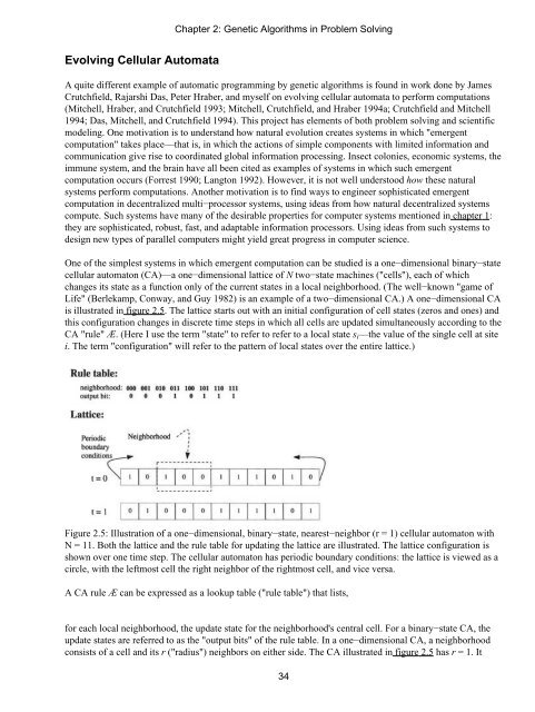The term "configuration" will refer to the pattern of local states over the entire lattice.) Figure 2.5: Illustration of a one−dimensional, binary−state, nearest−neighbor (r = 1) cellular automaton with N = 11. Both the lattice and the rule table for updating the lattice are illustrated. The lattice configuration is shown over one time step. The cellular automaton has periodic boundary conditions: the lattice is viewed as a circle, with the leftmost cell the right neighbor of the rightmost cell, and vice versa. A CA rule Æ can be expressed as a lookup table ("rule table") that lists, for each local neighborhood, the update state for the neighborhood's central cell. For a binary−state CA, the update states are referred to as the "output bits" of the rule table. In a one−dimensional CA, a neighborhood consists of a cell and its r ("radius") neighbors on either side. The CA illustrated in figure 2.5 has r = 1. It 34
Chapter 2: Genetic Algorithms in Problem Solving illustrates the "majority" rule: for each neighborhood of three adjacent cells, the new state is decided by a majority vote among the three cells. The CA illustrated in figure 2.5, like all those I will discuss here, has periodic boundary conditions: si = si + N. In figure 2.5 the lattice configuration is shown iterated over one time step. Cellular automata have been studied extensively as mathematical objects, as models of natural systems, and as architectures for fast, reliable parallel computation. (For overviews of CA theory and applications, see Toffoli and Margolus 1987 and Wolfram 1986.) However, the difficulty of understanding the emergent behavior of CAs or of designing CAs to have desired behavior has up to now severely limited their use in science and engineering and for general computation. Our goal is to use GAs as a method for engineering CAs to perform computations. Typically, a CA performing a computation means that the input to the computation is encoded as an initial configuration, the output is read off the configuration after some time step, and the intermediate steps that transform the input to the output are taken as the steps in the computation. The "program" emerges from the CA rule being obeyed by each cell. (Note that this use of CAs as computers differs from the impractical though theoretically interesting method of constructing a universal Turing machine in a CA; see Mitchell, Crutchfield, and Hraber 1994b for a comparison of these two approaches.) The behavior of one−dimensional CAs is often illustrated by a "space−time diagram"—a plot of lattice configurations over a range of time steps, with ones given as black cells and zeros given as white cells and with time increasing down the page. Figure 2.6 shows such a diagram for a binary−state r = 3 CA in which the rule table's output bits were filled in at random. It is shown iterating on a randomly generated initial configuration. Random−looking patterns, such as the one shown, are typical for the vast majority of CAs. To produce CAs that can perform sophisticated parallel computations, the genetic algorithm must evolve CAs in which the actions of the cells are not random−looking but are coordinated with one another so as to produce the desired result. This coordination must, of course, happen in the absence of any central processor or memory directing the coordination. Figure 2.6: Space−time diagram for a randomly generated r = 3 cellular automaton, iterating on a randomly generated initial configuration. N = 149 sites are shown, with time increasing down the page. Here cells with state 0 are white and cells with state 1 are black. (This and the other space−time diagrams given here were generated using the program "la1d" written by James P. Crutchfield.) 35
Page 2 and 3: An Introduction to Genetic Algorith
Page 4 and 5: Table of Contents Chapter 4: Theore
Page 6 and 7: Chapter 1: Genetic Algorithms: An O
Page 10 and 11: 1.4 SEARCH SPACES AND FITNESS LANDS
Page 12 and 13: potential energy is a measure of ho
Page 14 and 15: A simple method of implementing fit
Page 16 and 17: from an initial state to a goal. Fo
Page 18 and 19: Robert Axelrod of the University of
Page 26 and 27: instances of H at time t, and let
Page 28 and 29: What is the total payoff after 10 g
Page 30 and 31: 6. * c. d. a. b. Chapter 1: Genetic
Page 32 and 33: As a simple example, consider a pro
Page 34 and 35: Chapter 2: Genetic Algorithms in Pr
Page 36 and 37: it to get one fitness case correct:
Page 42 and 43: up most of the computation time. Ch
Page 46 and 47: the prospect of using GAs to automa
Page 48 and 49: where Ã is the standard deviation
Page 54 and 55: the brain. In a feedforward network
Page 58 and 59: Figure 2.21: An illustration of Mil
Page 62 and 63: experiments with grammatical encodi
Page 64 and 65: function of the average error of th
Page 66 and 67: COMPUTER EXERCISES 1. 2. 3. 4. 5. 6
Page 70 and 71: simulated generations, and such sim
Page 72 and 73: environments, they can fairly quick
Page 74 and 75: Chapter 3: Genetic Algorithms in Sc
Page 76 and 77: Figure 3.6: A schematic illustratio
Page 82 and 83: an initial population in which the
Page 88 and 89:
these random effects, Bedau and Pac
Page 90 and 91:
3. * 4. * the female child in the n
Page 92 and 93:
calculating the observed average fi
Page 94 and 95:
(4.1) The goal is to find n = n* th
Page 96 and 97:
competition in the d *···* parti
Page 98 and 99:
schemas with the best observed fitn
Page 100 and 101:
Steepest−ascent hill climbing (SA
Page 102 and 103:
(If the algorithm spends only 1/m o
Page 104 and 105:
strings—then in principle crossov
Page 106 and 107:
(4.7) Chapter 4: Theoretical Founda
Page 108 and 109:
2. 3. Calculate the fitness f(x) of
Page 110 and 111:
Defining ri,j(k) and is somewhat tr
Page 112 and 113:
Results of the Formalization How ca
Page 114 and 115:
Chapter 4: Theoretical Foundations
Page 116 and 117:
Page 118 and 119:
Figure 4.5: Predicted and observed
Page 120 and 121:
COMPUTER EXERCISES 1. 2. 3. 4. 5. 6
Page 122 and 123:
prone to rather arbitrary orderings
Page 124 and 125:
Inversion works by choosing two poi
Page 126 and 127:
Page 128 and 129:
The one hitch is that, as was seen
Page 130 and 131:
used in the work of Tanese (1989),
Page 132 and 133:
Two individuals are chosen at rando
Page 134 and 135:
Page 136 and 137:
strategies community, in which para
Page 138 and 139:
* 10. * 11. * 12. * Chapter 4: Theo
Page 140 and 141:
Chapter 6: Conclusions and Future D
Page 142 and 143:
Chapter 6: Conclusions and Future D
Page 144 and 145:
Appendix A: Selected General Refere
Page 146 and 147:
Evolution Artificielle Foundations
Page 148 and 149:
Kaufmann. Appendix B: Other Resourc
Page 150 and 151:
Morgan Kaufmann. Appendix B: Other
Page 152 and 153:
Appendix B: Other Resources Forrest
Page 154 and 155:
Appendix B: Other Resources Grefens
Page 156 and 157:
Kirkpatrick, S., Gelatt, C.D., Jr.,
Page 158 and 159:
Appendix B: Other Resources Mitchel
Page 160 and 161:
Appendix B: Other Resources Roughga
Page 162:
Appendix B: Other Resources Vose, M
show all

An Introduction to Genetic Algorithms - Boente

You also want an ePaper? Increase the reach of your titles

Delete template?

Save as template?