An Introduction to Genetic Algorithms - Boente

More documents

Recommendations

Info

Chapter 2: Genetic Algorithms in Problem Solving Some early work on evolving CAs with genetic algorithms was done by Norman Packard and his colleagues (Packard 1988; Richards, Meyer, and Packard 1990). John Koza (1992) also applied the GP paradigm to evolve CAs for simple random−number generation. Our work builds on that of Packard (1988). As a preliminary project, we used a form of the GA to evolve one−dimensional, binary−state r = 3 CAs to perform a density−classification task. The goal is to find a CA that decides whether or not the initial configuration contains a majority of ones (i.e., has high density). If it does, the whole lattice should eventually go to an unchanging configuration of all ones; all zeros otherwise. More formally, we call this task the task. Here Á denotes the density of ones in a binary−state CA configuration and Ác denotes a "critical" or threshold density for classification. Let Á0 denote the density of ones in the initial configuration (IC). If Á0 > Ác, then within M time steps the CA should go to the fixed−point configuration of all ones (i.e., all cells in state 1 for all subsequent t); otherwise, within M time steps it should go to the fixed−point configuration of all zeros. M is a parameter of the task that depends on the lattice size N. 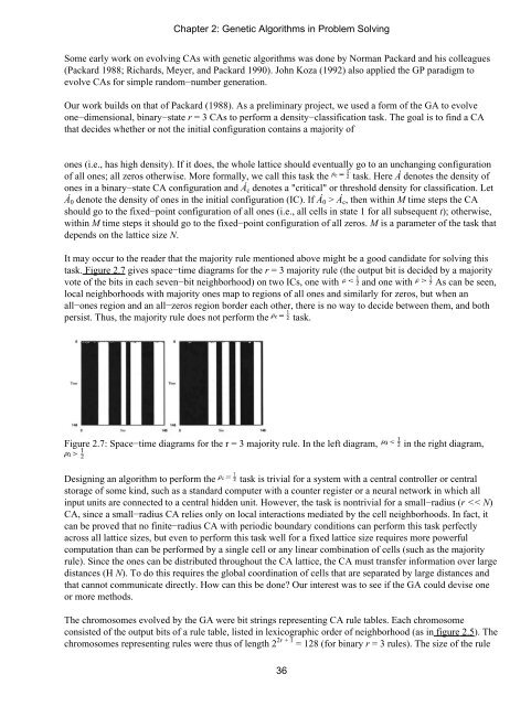It may occur to the reader that the majority rule mentioned above might be a good candidate for solving this task. Figure 2.7 gives space−time diagrams for the r = 3 majority rule (the output bit is decided by a majority vote of the bits in each seven−bit neighborhood) on two ICs, one with and one with As can be seen, local neighborhoods with majority ones map to regions of all ones and similarly for zeros, but when an all−ones region and an all−zeros region border each other, there is no way to decide between them, and both persist. Thus, the majority rule does not perform the task. Figure 2.7: Space−time diagrams for the r = 3 majority rule. In the left diagram, in the right diagram, Designing an algorithm to perform the task is trivial for a system with a central controller or central storage of some kind, such as a standard computer with a counter register or a neural network in which all input units are connected to a central hidden unit. However, the task is nontrivial for a small−radius (r
Chapter 2: Genetic Algorithms in Problem Solving space the GA searched was thus 2 128 —far too large for any kind of exhaustive search. In our main set of experiments, we set N = 149 (chosen to be reasonably large but not computationally intractable). The GA began with a population of 100 randomly generated chromosomes (generated with some initial biases—see Mitchell, Crutchfield, and Hraber 1994a, for details). The fitness of a rule in the population was calculated by (i) randomly choosing 100 ICs (initial configurations) that are uniformly distributed over Á Î [0.0,1.0], with exactly half with ÁÁc and half with ÁÁc, (ii) running the rule on each IC either until it arrives at a fixed point or for a maximum of approximately 2N time steps, and (iii) determining whether the final pattern is correct—i.e., N zeros for Á0Ác and N ones for Á0Ác. The initial density, Á0, was never exactly since N was chosen to be odd. The rule's fitness, f100, was the fraction of the 100 ICs on which the rule produced the correct final pattern. No partial credit was given for partially correct final configurations. A few comments about the fitness function are in order. First, as was the case in Hillis's sorting−networks project, the number of possible input cases (2 149 for N = 149) was far too large to test exhaustively. Instead, the GA sampled a different set of 100 ICs at each generation. In addition, the ICs were not sampled from an unbiased distribution (i.e., equal probability of a one or a zero at each site in the IC), but rather from a flat distribution across Á Î [0,1] (i.e., ICs of each density from Á = 0 to Á = 1 were approximately equally represented). This flat distribution was used because the unbiased distribution is binomially distributed and thus very strongly peaked at . The ICs selected from such a distribution will likely all have , the hardest cases to classify. Using an unbiased sample made it too difficult for the GA to ever find any high−fitness CAs. (As will be discussed below, this biased distribution turns out to impede the GA in later generations: as increasingly fit rules are evolved, the IC sample becomes less and less challenging for the GA.) Our version of the GA worked as follows. In each generation, (i) a new set of 100 ICs was generated, (ii) f100 was calculated for each rule in the population, (iii) the population was ranked in order of fitness, (iv) the 20 highest−fitness ("elite") rules were copied to the next generation without modification, and (v) the remaining 80 rules for the next generation were formed by single−point crossovers between randomly chosen pairs of elite rules. The parent rules were chosen from the elite with replacement—that is, an elite rule was permitted to be chosen any number of times. The offspring from each crossover were each mutated twice. This process was repeated for 100 generations for a single run of the GA. (More details of the implementation are given in Mitchell, Crutchfield, and Hraber 1994a.) Note that this version of the GA differs from the simple GA in several ways. First, rather than selecting parents with probability proportional to fitness, the rules are ranked and selection is done at random from the top 20% of the population. Moreover, all of the top 20% are copied without modification to the next generation, and only the bottom 80% are replaced. This is similar to the selection method—called "(¼ + »)"—used in some evolution strategies; see Back, Hoffmeister, and Schwefel 1991. This version of the GA was the one used by Packard (1988), so we used it in our experiments attempting to replicate his work (Mitchell, Hraber, and Crutchfield 1993) and in our subsequent experiments. Selecting parents by rank rather than by absolute fitness prevents initially stronger individuals from quickly dominating the population and driving the genetic diversity down too early. Also, since testing a rule on 100 ICs provides only an approximate gauge of the true fitness, saving the top 20% of the rules was a good way of making a "first cut" and allowing rules that survive to be tested over more ICs. Since a new set of ICs was produced every generation, rules that were copied without modification were always retested on this new set. If a rule performed well and thus survived over a large number of generations, then it was likely to be a genuinely better rule than those that were not selected, since it was tested with a large set of ICs. An alternative method would be to test every rule in each generation on a much larger set of ICs, but this would waste computation time. Too much effort, for example, would go into testing very weak rules, which can safely be weeded out early using our method. As in most applications, evaluating the fitness function (here, iterating each CA) takes 37
Page 2 and 3: An Introduction to Genetic Algorith
Page 4 and 5: Table of Contents Chapter 4: Theore
Page 6 and 7: Chapter 1: Genetic Algorithms: An O
Page 10 and 11: 1.4 SEARCH SPACES AND FITNESS LANDS
Page 12 and 13: potential energy is a measure of ho
Page 14 and 15: A simple method of implementing fit
Page 16 and 17: from an initial state to a goal. Fo
Page 18 and 19: Robert Axelrod of the University of
Page 26 and 27: instances of H at time t, and let
Page 28 and 29: What is the total payoff after 10 g
Page 30 and 31: 6. * c. d. a. b. Chapter 1: Genetic
Page 32 and 33: As a simple example, consider a pro
Page 34 and 35: Chapter 2: Genetic Algorithms in Pr
Page 36 and 37: it to get one fitness case correct:
Page 38 and 39: Evolving Cellular Automata Chapter
Page 42 and 43: up most of the computation time. Ch
Page 46 and 47: the prospect of using GAs to automa
Page 48 and 49: where Ã is the standard deviation
Page 54 and 55: the brain. In a feedforward network
Page 58 and 59: Figure 2.21: An illustration of Mil
Page 62 and 63: experiments with grammatical encodi
Page 64 and 65: function of the average error of th
Page 66 and 67: COMPUTER EXERCISES 1. 2. 3. 4. 5. 6
Page 70 and 71: simulated generations, and such sim
Page 72 and 73: environments, they can fairly quick
Page 74 and 75: Chapter 3: Genetic Algorithms in Sc
Page 76 and 77: Figure 3.6: A schematic illustratio
Page 82 and 83: an initial population in which the
Page 88 and 89: these random effects, Bedau and Pac
Page 90 and 91:
3. * 4. * the female child in the n
Page 92 and 93:
calculating the observed average fi
Page 94 and 95:
(4.1) The goal is to find n = n* th
Page 96 and 97:
competition in the d *···* parti
Page 98 and 99:
schemas with the best observed fitn
Page 100 and 101:
Steepest−ascent hill climbing (SA
Page 102 and 103:
(If the algorithm spends only 1/m o
Page 104 and 105:
strings—then in principle crossov
Page 106 and 107:
(4.7) Chapter 4: Theoretical Founda
Page 108 and 109:
2. 3. Calculate the fitness f(x) of
Page 110 and 111:
Defining ri,j(k) and is somewhat tr
Page 112 and 113:
Results of the Formalization How ca
Page 114 and 115:
Chapter 4: Theoretical Foundations
Page 116 and 117:
Page 118 and 119:
Figure 4.5: Predicted and observed
Page 120 and 121:
COMPUTER EXERCISES 1. 2. 3. 4. 5. 6
Page 122 and 123:
prone to rather arbitrary orderings
Page 124 and 125:
Inversion works by choosing two poi
Page 126 and 127:
Page 128 and 129:
The one hitch is that, as was seen
Page 130 and 131:
used in the work of Tanese (1989),
Page 132 and 133:
Two individuals are chosen at rando
Page 134 and 135:
Page 136 and 137:
strategies community, in which para
Page 138 and 139:
* 10. * 11. * 12. * Chapter 4: Theo
Page 140 and 141:
Chapter 6: Conclusions and Future D
Page 142 and 143:
Chapter 6: Conclusions and Future D
Page 144 and 145:
Appendix A: Selected General Refere
Page 146 and 147:
Evolution Artificielle Foundations
Page 148 and 149:
Kaufmann. Appendix B: Other Resourc
Page 150 and 151:
Morgan Kaufmann. Appendix B: Other
Page 152 and 153:
Appendix B: Other Resources Forrest
Page 154 and 155:
Appendix B: Other Resources Grefens
Page 156 and 157:
Kirkpatrick, S., Gelatt, C.D., Jr.,
Page 158 and 159:
Appendix B: Other Resources Mitchel
Page 160 and 161:
Appendix B: Other Resources Roughga
Page 162:
Appendix B: Other Resources Vose, M
show all

An Introduction to Genetic Algorithms - Boente

You also want an ePaper? Increase the reach of your titles

Delete template?

Save as template?