An Introduction to Genetic Algorithms - Boente

Chapter 2: Genetic Algorithms in Problem Solving
illustrates the "majority" rule: for each neighborhood of three adjacent cells, the new state is decided by a
majority vote among the three cells. The CA illustrated in figure 2.5, like all those I will discuss here, has
periodic boundary conditions: si = si + N. In figure 2.5 the lattice configuration is shown iterated over one time
step.
Cellular automata have been studied extensively as mathematical objects, as models of natural systems, and as
architectures for fast, reliable parallel computation. (For overviews of CA theory and applications, see Toffoli
and Margolus 1987 and Wolfram 1986.) However, the difficulty of understanding the emergent behavior of
CAs or of designing CAs to have desired behavior has up to now severely limited their use in science and
engineering and for general computation. Our goal is to use GAs as a method for engineering CAs to perform
computations.
Typically, a CA performing a computation means that the input to the computation is encoded as an initial
configuration, the output is read off the configuration after some time step, and the intermediate steps that
transform the input to the output are taken as the steps in the computation. The "program" emerges from the
CA rule being obeyed by each cell. (Note that this use of CAs as computers differs from the impractical
though theoretically interesting method of constructing a universal Turing machine in a CA; see Mitchell,
Crutchfield, and Hraber 1994b for a comparison of these two approaches.)
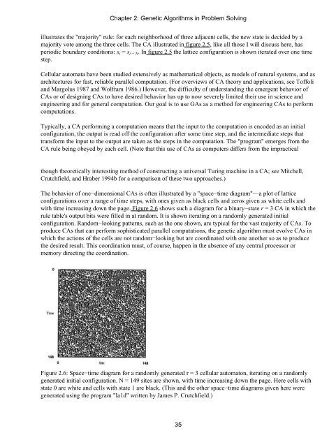
The behavior of one−dimensional CAs is often illustrated by a "space−time diagram"—a plot of lattice
configurations over a range of time steps, with ones given as black cells and zeros given as white cells and
with time increasing down the page. Figure 2.6 shows such a diagram for a binary−state r = 3 CA in which the
rule table's output bits were filled in at random. It is shown iterating on a randomly generated initial
configuration. Random−looking patterns, such as the one shown, are typical for the vast majority of CAs. To
produce CAs that can perform sophisticated parallel computations, the genetic algorithm must evolve CAs in
which the actions of the cells are not random−looking but are coordinated with one another so as to produce
the desired result. This coordination must, of course, happen in the absence of any central processor or
memory directing the coordination.
Figure 2.6: Space−time diagram for a randomly generated r = 3 cellular automaton, iterating on a randomly
generated initial configuration. N = 149 sites are shown, with time increasing down the page. Here cells with
state 0 are white and cells with state 1 are black. (This and the other space−time diagrams given here were
generated using the program "la1d" written by James P. Crutchfield.)
35