Coda wave interferometry - Inside Mines
Coda wave interferometry - Inside Mines
Coda wave interferometry - Inside Mines

Create successful ePaper yourself
Turn your PDF publications into a flip-book with our unique Google optimized e-Paper software.
<strong>Coda</strong> <strong>wave</strong> <strong>interferometry</strong><br />
An interferometer is an instrument that is sensitive<br />
to the interference of two or more <strong>wave</strong>s (optical<br />
or acoustic). For example, an optical interferometer<br />
uses two interfering light beams to measure small<br />
length changes.<br />
<strong>Coda</strong> <strong>wave</strong> <strong>interferometry</strong> is a technique for monitoring<br />
changes in media over time using acoustic<br />
or elastic <strong>wave</strong>s. Sound <strong>wave</strong>s that travel through<br />
a medium are scattered multiple times by heterogeneities<br />
in the medium and generate slowly decaying<br />
(late-arriving) <strong>wave</strong> trains, called coda <strong>wave</strong>s.<br />
Despite their noisy and chaotic appearance, coda<br />
<strong>wave</strong>s are highly repeatable such that if no change<br />
occurs in the medium over time, the <strong>wave</strong>forms are<br />
identical. If a change occurs, such as a crack in the<br />
medium, the change in the multiple scattered <strong>wave</strong>s<br />
will result in an observable change in the coda <strong>wave</strong>s.<br />
<strong>Coda</strong> <strong>wave</strong> <strong>interferometry</strong> uses this sensitivity to<br />
monitor temporal changes in strongly scattering<br />
media.<br />
There are many potential applications of coda<br />
<strong>wave</strong> <strong>interferometry</strong>. In geotechnical applications,<br />
the technique can be used to monitor dams or tunnel<br />
roofs. In nondestructive testing, the technique can<br />
be used to monitor changes due to the formation of<br />
cracks or other changes in materials. In hazard monitoring,<br />
the technique can be used to monitor volcanoes,<br />
fault zones, or landslide areas. In the context<br />
of the “intelligent oilfield,” coda <strong>wave</strong> <strong>interferometry</strong><br />
can be used to monitor changes in hydrocarbon<br />
reservoirs during production.<br />
<strong>Coda</strong> <strong>wave</strong> <strong>interferometry</strong> can be used in two different<br />
modes. In the warning mode, the technique<br />
is used to detect a change in the medium, but this<br />
change is not quantified. This mode of operation is<br />
used to prompt further action, such as more elaborate<br />
diagnostics. In the diagnostic mode, coda <strong>wave</strong><br />
<strong>interferometry</strong> is used to quantify the change in the<br />
medium.<br />
Volcano monitoring. The use of this technique to<br />
detect changes in a medium can be illustrated with<br />
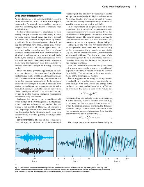
1998<br />
E- - - L- - -<br />
1997<br />
0 10<br />
time, s<br />
(a)<br />
1.5 2 2.5<br />
time, s<br />
3 3.5<br />
(b)<br />
seismological data that have been recorded on the<br />
Merapi volcano in Java by U. Wegler and coworkers.<br />
As seismic (elastic) <strong>wave</strong>s pass through a volcano,<br />
they are scattered by heterogeneities (scatters) such<br />
as voids, cracks, magma bodies, and faults.<br />
In the experiment, an air gun placed in a small<br />
water basin dug in the side of the volcano was used<br />
to generate seismic <strong>wave</strong>s. (An air gun is a device that<br />
emits a bubble of compressed air in water as a source<br />
of seismic <strong>wave</strong>s.) The seismic <strong>wave</strong>s generated by<br />
the same source recorded at a fixed receiver at two<br />
moments in time (a year apart) are shown in Fig. 1.<br />
In the Fig. 1b and c, the two <strong>wave</strong>forms are shown<br />
superimposed in more detail. For the interval early<br />
in the seismogram, these <strong>wave</strong>forms are similar<br />
(Fig. 1b). For the later interval (coda), the <strong>wave</strong>forms<br />
are distinctly different (Fig. 1c), where one of the<br />
<strong>wave</strong>forms appears to be a time-shifted version of<br />
the other, indicating that the interior of the volcano<br />
had changed over time.<br />
Note that in coda <strong>wave</strong> <strong>interferometry</strong> one needs<br />
only a single source and a single receiver, although<br />
in practice one may use more receivers to increase<br />
the reliability. This means that the hardware requirements<br />
of this technique are modest.<br />
Theory. Suppose that a strongly scattering medium<br />
is excited by a repeatable source, and that the medium<br />
changes with time. Before the change in the<br />
medium, the unperturbed <strong>wave</strong> field u (u) (t) can<br />
be written in Eq. (1) as a sum of the <strong>wave</strong>s that<br />
u (u) (t) = �<br />
AT (t) (1)<br />
propagate along the multiple scattering trajectories<br />
T in the medium, where t denotes time and AT (t)<br />
is the <strong>wave</strong> that has propagated along trajectory T.<br />
When the medium changes over time, the dominant<br />
effect is a change τ T in the arrival times of the <strong>wave</strong>s<br />
that propagate along each trajectory T, so that the<br />
perturbed <strong>wave</strong> field is given by Eq. (2).<br />
u (p) (t) = �<br />
AT (t − τT ) (2)<br />
Fig. 1. Waveforms recorded at the Merapi volcano for the same source and receiver on July 1997 (black) and July 1998<br />
(color). (a) Complete <strong>wave</strong>forms and definition of the early (E) and late (L) time interval. (b) The recorded <strong>wave</strong>s in the early<br />
time interval (E). (c) The recorded <strong>wave</strong>s in the later interval (L). (Data courtesy of Ulrich Wegler)<br />
E<br />
T<br />
The change in the <strong>wave</strong>forms as shown in Fig. 1c<br />
T<br />
(c)<br />
<strong>Coda</strong> <strong>wave</strong> <strong>interferometry</strong> 1<br />
12.5 13<br />
time, s<br />
13.5<br />
L
2 <strong>Coda</strong> <strong>wave</strong> <strong>interferometry</strong><br />
(a)<br />
|dv/v|<br />
(b)<br />
1.5<br />
0.5<br />
−0.5<br />
−1.5<br />
0.003<br />
0.002<br />
0.001<br />
can be quantified by computing in Eq. (3) the time-<br />
� t+tw<br />
t−tw<br />
R(ts) ≡<br />
u(u) (t ′ )u ( p) (t ′ + ts) dt ′<br />
� � t+tw<br />
t−tw u(u)2 (t ′ ) dt ′ � t+tw<br />
t−tw u(p)2 (t ′ ) dt ′<br />
� (3) 1/2<br />
shifted cross-correlation over a time window with<br />
center time t and width 2tw, where ts is the time<br />
shift of the perturbed <strong>wave</strong>form relative to the unperturbed<br />
<strong>wave</strong>form. Suppose that the <strong>wave</strong>s are not<br />
perturbed. In that case, u (p) (t) = u (u) (t) and the timeshifted<br />
cross-correlation is equal to unity for a zero<br />
lag time R(ts = 0) = 1. When the perturbed <strong>wave</strong><br />
is a time-shifted version of the original <strong>wave</strong>, then<br />
u (p) (t) = u (u) (t − τ) and R(ts) attain its maximum for<br />
ts = τ.<br />
In general, the time-shifted cross-correlation R(ts)<br />
attains its maximum at a time ts = tmax [Eq. (4)] when<br />
tmax =〈τ〉 (4)<br />
the shift time is given by the average perturbation of<br />
the travel time of the <strong>wave</strong>s that arrive in the employed<br />
time window, and the value Rmax at its maximum<br />
[Eq. (5)] is related to the variance σ τ of the<br />
R (t,tw)<br />
max<br />
1<br />
= 1 −<br />
2 ω2σ 2<br />
τ<br />
(5)<br />
travel-time perturbation of the <strong>wave</strong>s that arrive in<br />
the time window, where ω is the angular frequency<br />
of the <strong>wave</strong>s. Given the recorded <strong>wave</strong>forms before<br />
and after the perturbation, one can readily compute<br />
the time-shifted cross-correlation and use Eqs. (4)<br />
and (5) to obtain the mean and the variance of the<br />
travel-time perturbation in the medium.<br />
0.000<br />
0.0 0.5 1.0<br />
time, ms<br />
1.5 2.0<br />
Fig. 2. Measuring velocity change. (a) Ultrasound <strong>wave</strong>s were recorded in a small granite<br />
sample. (b) The relative velocity change for a 5 ◦ C(9 ◦ F) increase in temperature as a<br />
function of the center time of each time window was used to measure the velocity change.<br />
Measuring velocity change. Figure 2a shows an experiment<br />
in which ultrasound <strong>wave</strong>s were propagated<br />
through a granite cylinder and recorded. The<br />
<strong>wave</strong>s are complex due to the reverberations within<br />
this cylinder. With a heating coil, the temperature<br />
of the cylinder was raised 5 ◦ C(9 ◦ F). The perturbed<br />
<strong>wave</strong>forms have the same character as the unperturbed<br />
<strong>wave</strong>s shown in Fig. 2a. The tail of the <strong>wave</strong><br />
trains was divided in 15 nonoverlapping time intervals.<br />
For each time interval, the time shift between<br />
the perturbed and unperturbed <strong>wave</strong>s was determined<br />
by computing the time-shifted crosscorrelation<br />
of Eq. (3) and by picking the time for<br />
which it attains its maximum tmax. The relative<br />
velocity change for each time interval is given by<br />
δv/v =−tmax/t. This quantity is shown in Fig. 2b as<br />
a function of the center time of the employed time<br />
windows.<br />
Since the employed time windows are nonoverlapping,<br />
the measurements of the velocity change in the<br />
different time windows are independent. The scatter<br />
in the different estimates of the velocity change is<br />
small; this provides a consistency check of coda <strong>wave</strong><br />
<strong>interferometry</strong>. The variability in the measurements<br />
can be used to estimate the error in the velocity<br />
change. Note that the relative velocity change in<br />
this example is only about 0.16% with an error of<br />
about 0.03%. This extreme sensitivity to changes in<br />
the medium is due to the sensitivity of the multiply<br />
scattered <strong>wave</strong>s to changes in the granite.<br />
In an elastic medium such as granite, there is no<br />
single <strong>wave</strong> velocity. Compressional (P) <strong>wave</strong>s and<br />
shear (S) <strong>wave</strong>s propagate with different velocities<br />
vP and vS, respectively. The change in the velocity<br />
inferred from coda <strong>wave</strong> <strong>interferometry</strong> [Eq. (6)] is a<br />
δv<br />
v =<br />
v 3 S<br />
2v 3 P + v 3 S<br />
δvP<br />
vP<br />
+ 2v3 P<br />
2v 3 P + v 3 S<br />
δvS<br />
vS<br />
(6)<br />
weighted average of the change in the velocities for<br />
the two <strong>wave</strong> types. For a Poisson medium, an elastic<br />
medium, where vP = √ 3vS, the relative velocity<br />
change is given by δv/v ≈ 0.09δvP/vP + 0.91δvS/vS.<br />
This means that in practice coda <strong>wave</strong> <strong>interferometry</strong><br />
provides a constraint on the change in the shear<br />
velocity vS.<br />
Other applications. Some applications may involve<br />
a change in the location of scatterers, or a change<br />
in the source position. This can be used to monitor<br />
the properties of a turbulent fluid. One can seed<br />
the fluid with neutrally buoyant particles that scatter<br />
<strong>wave</strong>s. Acoustic <strong>wave</strong>s that propagate through the<br />
fluid are scattered by these particles. Over time, the<br />
particles are swept along by the turbulent motion.<br />
When acoustic <strong>wave</strong>s are sent into the fluid once<br />
more from the same source, the <strong>wave</strong>s are scattered<br />
by particles that have been displaced by the turbulent<br />
flow. The resulting change in the recorded <strong>wave</strong>s<br />
can be used to characterize the properties of the turbulent<br />
flow.<br />
<strong>Coda</strong> <strong>wave</strong> <strong>interferometry</strong>, to a certain extent,<br />
can be used to distinguish between different
Imprint of different type of changes on the mean 〈τ〉 and<br />
the variance of the travel-time perturbation<br />
σ 2 τ<br />
Type of change<br />
Change in velocity t 0<br />
Movement of scatterers 0 t<br />
Displaced source 0 Constant<br />
perturbations. When the velocity changes, the mean<br />
travel-time perturbation is nonzero and is proportional<br />
to the total travel time. Since the <strong>wave</strong>s that<br />
propagate along all paths experience the same traveltime<br />
change, the variance of the travel-time<br />
perturbation vanishes. When the location of the scatterers<br />
is perturbed randomly, the mean travel-time<br />
perturbation vanishes, because some paths are<br />
longer, while others are shorter. However, the variance<br />
of the travel-time perturbation is nonzero and<br />
can be shown to grow linearly with time. When the<br />
source is displaced, the mean travel-time perturbation<br />
vanishes, and the variance of the travel time is<br />
constant with time. These results are summarized in<br />
〈τ〉<br />
σ 2 τ<br />
the table. The mean and the variance of the traveltime<br />
change can be computed from the unperturbed<br />
and the perturbed <strong>wave</strong>forms. Since different types<br />
of perturbations leave a different imprint on these<br />
quantities, coda <strong>wave</strong> <strong>interferometry</strong> can help determine<br />
the mechanism of the change over time.<br />
For background information see ACOUSTIC EMIS-<br />
SION; ACOUSTICS; EARTHQUAKE; INTERFEROMETRY;<br />
SEISMOGRAPHIC INSTRUMENTATION; SEISMOLOGY;<br />
SOUND; VOLCANO; VOLCANOLOGY in the McGraw-<br />
Hill Encyclopedia of Science & Technology.<br />
Roel Snieder<br />
Bibliography. R. Snieder, <strong>Coda</strong> <strong>wave</strong> <strong>interferometry</strong><br />
and the equilibration of energy in elastic media,<br />
Phys. Rev. E, 66:046615–1,8, 2002; R. Snieder<br />
et al., <strong>Coda</strong> <strong>wave</strong> <strong>interferometry</strong> for estimating nonlinear<br />
behavior in seismic velocity, Science, 295:<br />
2253–2255, 2002; R. Snieder and J. A. Scales, Time<br />
reversed imaging as a diagnostic of <strong>wave</strong> and particle<br />
chaos, Phys. Rev. E, 58:5668–5675, 1998; U. Wegler,<br />
B. G. Luhr, and A. Ratdomopurbo, A repeatable seismic<br />
source for tomography at volcanoes, Ann. Geofisica,<br />
42:565–571, 1999.<br />
Reprinted from the McGraw-Hill Yearbook of Science &<br />
Technology 2004. c○ Copyright 2004 by The McGraw-<br />
Hill Companies, Inc. All rights reserved.<br />
<strong>Coda</strong> <strong>wave</strong> <strong>interferometry</strong> 3