An Introduction to Iterative Learning Control - Inside Mines
An Introduction to Iterative Learning Control - Inside Mines
An Introduction to Iterative Learning Control - Inside Mines

Create successful ePaper yourself
Turn your PDF publications into a flip-book with our unique Google optimized e-Paper software.
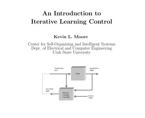
<strong>An</strong> <strong>Introduction</strong> <strong>to</strong><br />
<strong>Iterative</strong> <strong>Learning</strong> <strong>Control</strong><br />
Kevin L. Moore<br />
Center for Self-Organizing and Intelligent Systems<br />
Dept. of Electrical and Computer Engineering<br />
Utah State University
• <strong>Introduction</strong><br />
Outline<br />
• <strong>Control</strong> System Design: Motivation for ILC<br />
• <strong>Iterative</strong> <strong>Learning</strong> <strong>Control</strong>: The Basic Idea<br />
• A Short His<strong>to</strong>ry of ILC<br />
• ILC Problem Formulation<br />
• LTI ILC: Opera<strong>to</strong>r-Theoretic Approach<br />
• ILC as a 2-D Problem<br />
• Multi-Loop <strong>Control</strong> Approach <strong>to</strong> ILC<br />
• Higher-Order ILC: A Matrix Fraction Approach<br />
• More on the Nature of the ILC Solution: Equivalence of ILC <strong>to</strong><br />
One-Step Ahead <strong>Control</strong><br />
• Conclusion
<strong>Control</strong> Design Problem<br />
Reference Error Input Output<br />
<strong>Control</strong>ler<br />
System <strong>to</strong> be<br />
controlled<br />
Given: System <strong>to</strong> be controlled.<br />
Find: <strong>Control</strong>ler (using feedback).<br />
Such that: 1) Closed-loop system is stable.<br />
2) Steady-state error is acceptable.<br />
3) Transient response is acceptable.
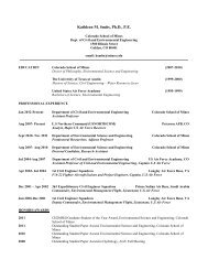
Motivation for the Problem of <strong>Iterative</strong> <strong>Learning</strong> <strong>Control</strong><br />
• Transient response design is hard:<br />
1) Robustness is always an issue:<br />
- Modelling uncertainty.<br />
- Parameter variations.<br />
- Disturbances.<br />
2) Lack of theory (design uncertainty):<br />
0<br />
0 10 20 30 40 50 60 70<br />
- Relation between pole/zero locations and transient response.<br />
- Relation between Q/R weighting matrices in optimal control and transient<br />
response.<br />
- Nonlinear systems.<br />
• Many systems of interest in applications are operated in a repetitive fashion.<br />
• <strong>Iterative</strong> <strong>Learning</strong> <strong>Control</strong> (ILC) is a methodology that tries <strong>to</strong> address the<br />
problem of transient response performance for systems that operate repetitively.<br />
2.5<br />
2<br />
1.5<br />
1<br />
0.5
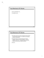
Systems that Execute the Same Trajec<strong>to</strong>ry Repetitively<br />
Step 1: Robot at rest, waiting for workpiece.<br />
Step 2: Workpiece moved in<strong>to</strong> position.<br />
Step 3: Robot moves <strong>to</strong> desired<br />
location<br />
Step 4: Robot returns <strong>to</strong> rest and<br />
waits for next workpiece.
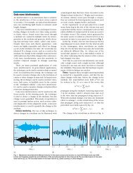
Errors are Repeated When<br />
Trajec<strong>to</strong>ries are Repeated<br />
•A typical joint angle trajec<strong>to</strong>ry for the example might look like this:<br />
2<br />
1.5<br />
1<br />
0.5<br />
0<br />
-0.5<br />
0 5 10 15 20 25 30<br />
•Each time the system is operated it will see the same overshoot,<br />
rise time, settling time, and steady-state error.<br />
•<strong>Iterative</strong> learning control attempts <strong>to</strong> improve the transient response by<br />
adjusting the input <strong>to</strong> the plant during future system operation based<br />
on the errors observed during past operation.
<strong>Iterative</strong> <strong>Learning</strong> <strong>Control</strong> - 1<br />
• Standard iterative learning control scheme:<br />
uk<br />
� ✲ System<br />
�<br />
✲<br />
Memory Memory Memory<br />
uk+1<br />
✻<br />
✻<br />
❄<br />
❄<br />
<strong>Learning</strong><br />
<strong>Control</strong>ler<br />
✛<br />
✛<br />
❄<br />
yk<br />
yd
<strong>Iterative</strong> <strong>Learning</strong> <strong>Control</strong> - 2<br />
• A typical ILC algorithm has the form:<br />
• Conventional feedback control has the form:<br />
• Standard ILC assumptions include:<br />
uk+1(t) = uk(t) + f(ek(t + 1))<br />
uk+1(t) = f(ek+1(t − 1))<br />
– Stable dynamics or some kind of Lipschitz condition.<br />
– System returns <strong>to</strong> the same initial conditions at the start of each trial.<br />
– Each trial has the same length.
• Consider the plant:<br />
A Simple Linear Example - 1<br />
y(t + 1) = −.7y(t) − .012y(t − 1) + u(t)<br />
y(0) = 2<br />
y(1) = 2<br />
• We wish <strong>to</strong> force the system <strong>to</strong> follow a signal yd:
• Use the following ILC procedure:<br />
1. Let<br />
2. Run the system<br />
3. Compute<br />
4. Let<br />
5. Iterate<br />
A Simple Linear Example - 2<br />
u0(t) = yd(t)<br />
e0(t) = yd(t) − y0(t)<br />
u1(t) = u0(t) + 0.5e0(t + 1)<br />
• Each iteration shows an improvement in tracking performance (plot shows desired and actual<br />
output on first, 5th, and 10th trials and input on 10th trial).
Adaptive ILC for a Robotic Manipula<strong>to</strong>r - 1<br />
• Consider a simple two-link manipula<strong>to</strong>r modelled by:<br />
where<br />
A(xk)¨xk + B(xk, ˙xk) ˙xk + C(xk) = uk<br />
x(t) = (θ1(t), θ2(t)) T<br />
� �<br />
.54 + .27 cos θ2 .135 + .135 cos θ2<br />
A(x) =<br />
.135 + .135 cos θ2 .135<br />
�<br />
.135 sin θ2 0<br />
B(x, ˙x) =<br />
−.27 sin θ2 −.135(sin θ2) ˙ �<br />
θ2<br />
� �<br />
13.1625 sin θ1 + 4.3875 sin(θ1 + θ2)<br />
C(x) =<br />
4.3875 sin(θ1 + θ2)<br />
uk(t) = vec<strong>to</strong>r of <strong>to</strong>rques applied <strong>to</strong> the joints<br />
g<br />
■<br />
✠<br />
�<br />
■<br />
✠<br />
���❍ m1 ❄ ✈ θ2<br />
❍<br />
❍❍❍❍<br />
✘l1<br />
l2 ✈m2<br />
�<br />
✙θ1<br />
l1 = l2 = 0.3m<br />
m1 = 3.0kg<br />
m2 = 1.5kg
Adaptive ILC for a Robotic Manipula<strong>to</strong>r - 2<br />
• Define the vec<strong>to</strong>rs:<br />
• The learning controller is defined by:<br />
yk = (x T k , ˙xT k , ¨xT k )T<br />
yd = (x T d , ˙xT d , ¨xT d )T<br />
uk = rk − αkΓyk + C(xd(0))<br />
rk+1 = rk + αkΓek<br />
αk+1 = αk + γ�ek� m<br />
• Γ is a fixed feedback gain matrix that has been made time-varying through the multiplication<br />
by the gain αk.<br />
• rk can be described as a time-varying reference input. rk(t) and adaptation of αk are<br />
effectively the ILC part of the algorithm.<br />
• With this algorithm we have combined conventional feedback with iterative learning control.
Adaptive ILC for a Robotic Manipula<strong>to</strong>r - 3<br />
• The basic idea of the algorithm:<br />
– Make αk larger at each trial by adding a positive number that is linked <strong>to</strong> the norm of<br />
the error.<br />
– When the algorithm begins <strong>to</strong> converge, the gain αk will eventually s<strong>to</strong>p growing.<br />
– The convergence proof depends on a high-gain feedback result.<br />
• To simulate this ILC algorithm for the two-joint manipula<strong>to</strong>r described above we used firs<strong>to</strong>rder<br />
highpass filters of the form<br />
H(s) = 10s<br />
s + 10<br />
<strong>to</strong> estimate the joint accelerations ¨ θ1 and ¨ θ2 from the joint velocities ˙ θ1 and ˙ θ2, respectively.<br />
• The gain matrix Γ = [P L K] used in the feedback and learning control law was defined by:<br />
P =<br />
�<br />
50.0 0<br />
�<br />
0 50.0<br />
L =<br />
�<br />
65.0 0<br />
�<br />
0 65.0<br />
K =<br />
� �<br />
2.5 0<br />
0 2.5<br />
• The adaptive gain adjustment in the learning controller uses γ = .1 and α0 is initialized <strong>to</strong><br />
0.01.<br />
• Each iteration shows an improvement in tracking performance.
A Short Overview of ILC - 1<br />
• His<strong>to</strong>rical Roots of ILC go back about twenty-five years:<br />
– Idea of a “multipass” system studied by Owens and Rogers in mid- <strong>to</strong> late-1970’s, with<br />
several resulting monographs.<br />
– <strong>Learning</strong> control concept introduced (in Japanese) by Uchiyama in 1978.<br />
– Pioneering work of Arimo<strong>to</strong>, et al. 1984-present.<br />
– Related research in repetitive and periodic control.<br />
– 1993 Springer monograph had about 90 ILC references.<br />
– 1997 Asian <strong>Control</strong> Conference had 30 papers on ILC (out of 600 papers presented at<br />
the meeting) and the first panel session on this <strong>to</strong>pic.<br />
– 1998 survey paper has about 250 ILC references.<br />
– Web-based online, searchable bibliographic database maintained by Yangquan Chen<br />
has about 500 references (see http://cicserver.ee.nus.edu.sg/ ilc).<br />
– ILC Workshop and Roundtable and three devoted sessions at 1998 CDC.<br />
– Edited book by Bien and Xu resulting from 1997 ASCC.<br />
– At least four Ph.D. dissertations on ILC since 1998.<br />
– Springer monograph by Chen and Wen, 1999.<br />
– Special sessions at 2000 ASCC, ICARV 2000, and 2nd Int. Conference on nD Systems.<br />
– Tu<strong>to</strong>rial at ICARV 200 and first CDC Tu<strong>to</strong>rial Workshop; first IFAC World Congress<br />
special session.<br />
– ILC Summer School at Utah State University, June 2003.
A Short Overview of ILC - 2<br />
• Past work in the field demonstrated the usefulness and applicability of the concept of ILC:<br />
– Linear systems.<br />
– Classes of nonlinear systems.<br />
– Applications <strong>to</strong> robotic systems.<br />
• Present status of the field reflects the continuing efforts of researchers <strong>to</strong>:<br />
– Develop design <strong>to</strong>ols.<br />
– Extend earlier results <strong>to</strong> broader classes of systems.<br />
– Realize a wider range of applications.<br />
– Understand and interpret ILC in terms of other control paradigms and in the larger<br />
context of learning in general.
• Systems:<br />
A Partial Classification of ILC Research<br />
– Open-loop vs. closed-loop.<br />
– Discrete-time vs. continuous-time.<br />
– Linear vs. nonlinear.<br />
– Time-invariant or time-varying.<br />
– Relative degree 1 vs. higher relative degree.<br />
– Same initial state vs. variable initial state.<br />
– Presence of disturbances.<br />
• Update algorithm:<br />
– Linear ILC vs. nonlinear ILC.<br />
– First-order ILC vs. higher-order.<br />
– Current cycle vs. past cycle.<br />
– Fixed ILC or adaptive ILC.<br />
– Time-domain vs. frequency analysis.<br />
– <strong>An</strong>alysis vs. design.<br />
– Assumptions on plant knowledge.<br />
• Applications: robotics, chemical processing, mechatronic systems.
ILC Problem Formulation - 1<br />
• Standard iterative learning control scheme:<br />
uk<br />
� ✲ System � ✲<br />
Memory Memory Memory<br />
uk+1<br />
✻<br />
✻<br />
❄<br />
❄<br />
<strong>Learning</strong><br />
<strong>Control</strong>ler<br />
• Goal: Find a learning control algorithm<br />
so that for all t ∈ [0, tf]<br />
✛<br />
✛<br />
❄<br />
uk+1(t) = fL(uk(t); yk(t), yd(t))<br />
lim<br />
k→∞ yk(t) = yd(t)<br />
yk<br />
yd
• Given<br />
• Find<br />
• So that<br />
ILC Problem Formulation - 2<br />
– a system S (possibly nonlinear, time-varying), with<br />
yk(t) = fSk (uk(t))<br />
– a desired response yd(t), defined on the interval (t0, tf).<br />
– a system L (possibly unknown, non-linear, time-varying).<br />
– the sequence of inputs produced by the iteration<br />
• Such that<br />
converges <strong>to</strong> a fixed point u ∗ .<br />
uk+1(t) = fLk (uk, yk, yd) = fLk (uk, fSk (uk), yd)<br />
lim<br />
k→∞ �yd − yk� = �yd − Tsu ∗ �<br />
is minimum on the interval (t0, tf) over all possible systems L, for a specified norm.<br />
• Linear case: uk+1 = Tuuk + Te(yd − yk)
Some <strong>Learning</strong> <strong>Control</strong> Algorithms<br />
• Arimo<strong>to</strong> first proposed a learning control algorithm of the form:<br />
Convergence is assured if �I − CBΓ�i < 1.<br />
uk+1(t) = uk(t) + Γ ˙ek(t)<br />
• Arimo<strong>to</strong> has also considered more general algorithms of the form:<br />
�<br />
uk+1 = uk + Φek + Γ ˙ek + Ψ ekdt<br />
• Various researchers have used gradient methods <strong>to</strong> optimize the gain Gk in:<br />
uk+1(t) = uk(t) + Gkek(t + 1)<br />
• It is also useful for design <strong>to</strong> specify the learning control algorithm in the frequency domain,<br />
for example:<br />
Uk+1(s) = L(s)[Uk(s) + aEk(s)]<br />
• Many schemes in the literature can be classified with one of the algorithms given above.
LTI ILC Convergence Conditions - 1<br />
• Theorem: For the plant yk = Tsuk, the linear time-invariant learning control algorithm<br />
converges <strong>to</strong> a fixed point u ∗ (t) given by<br />
with a final error<br />
defined on the interval (t0, tf) if<br />
• Observation:<br />
uk+1 = Tuuk + Te(yd − yk)<br />
u ∗ (t) = (I − Tu + TeTs) −1 Teyd(t)<br />
e ∗ (t) = lim<br />
k→∞ (yk − yd) = (I − Ts(I − Tu + TeTs) −1 Te)yd(t)<br />
�Tu − TeTs�i < 1<br />
– If Tu = I then �e ∗ (t)� = 0 for all t ∈ [<strong>to</strong>, tf].<br />
– Otherwise the error will be non-zero.
• General linear algorithm:<br />
• Can show that, if<br />
LTI ILC Convergence Conditions - 2<br />
(i) Tu = I and �I − TeTs�i < 1, then<br />
(ii) Tu �= I and �Tu − TeTs�i < 1, then<br />
uk+1(t) = Tuuk(t) + Te(yd(t) − yk(t))<br />
e ∗ (t) = lim<br />
k→∞ (yd(t) − yk(t)) = 0<br />
e ∗ (t) = (I − Ts(I − Tu + TeTs) −1 Te)yd(t) �= 0<br />
• Note: The convergence condition for (i) can require system invertibility.<br />
e.g., For convergence in the space of finite-energy signals, with a requirement that our ILC<br />
filters be causal, (i) holds only for those systems whose transfer functions are non-minimum<br />
phase and have no zeros at infinity.
LTI ILC - Convergence with Zero Error<br />
• Let Tu = I <strong>to</strong> get e ∗ (t) = 0 over the entire interval.<br />
• Condition for convergence becomes:<br />
• Unfortunately, this can be overly restrictive.<br />
• Example:<br />
If u ∈ U = L r 2 (0, ∞) and y ∈ Y = Lm 2<br />
However, we can easily show:<br />
�I − HeHs�i < 1<br />
(0, ∞) then the condition for convergence is:<br />
�I − He(s)Hs(s)�∞ < 1<br />
Theorem: There exists a proper, stable, LTI system He(s) ∈ H∞ such that<br />
�I − He(s)Hs(s)�∞ < 1<br />
if and only if Hs(s) is invertible over the space H∞.
LTI <strong>Learning</strong> <strong>Control</strong> - Nature of the Solution<br />
• Question: Given Ts, how do we pick Tu and Te <strong>to</strong> make the final error e ∗ (t) as “small” as<br />
possible, for the general linear ILC algorithm:<br />
• <strong>An</strong>swer: Let T ∗ n solve the problem:<br />
uk+1(t) = Tuuk(t) + Te(yd(t) − yk(t))<br />
min �(I − TsTn)yd�<br />
Tn<br />
It turns out that we can specify Tu and Te in terms of T ∗ n and the resulting learning controller<br />
converges <strong>to</strong> an optimal system input given by:<br />
u ∗ (t) = T ∗ nyd(t)<br />
• Conclusion:The essential effect of a properly designed learning controller is <strong>to</strong> produce the<br />
output of the best possible inverse of the system in the direction of yd.
LTI ILC - Convergence with Non-Zero Error<br />
• OPT1: Let uk ∈ U, yd, yk ∈ Y and Ts, Tu, Te ∈ X. Then given yd and Ts, find T ∗ u and T ∗ e<br />
that solve<br />
min<br />
Tu,Te∈X �(I − Ts(I − Tu + TeTs) −1 Te)yd�<br />
subject <strong>to</strong> �Tu − TeTs�i < 1.<br />
• OPT2: Let yd ∈ Y and let Tn, Ts ∈ X. Then given yd and Ts, find T ∗ n that solve<br />
min �(I − TsTn)yd�<br />
Tn∈X<br />
• Theorem: Let T ∗ n be the solution of OPT2. Fac<strong>to</strong>r T ∗ n = T ∗ mT ∗ e where T ∗−1<br />
m ∈ X and<br />
�I − T ∗−1<br />
m �i < 1. Define T ∗ u = I − T ∗−1<br />
m + T ∗ e Ts. Then T ∗ u and T ∗ e are the solution of OPT1.<br />
• If we plug these in<strong>to</strong> the expression for the fixed-point of the input <strong>to</strong> the system we find:<br />
u ∗ (t) = T ∗ nyd(t)<br />
• Note: The fac<strong>to</strong>rization in the Theorem can always be done, with the result that<br />
u ∗ (t) = T ∗ nyd(t).
Interlude: The Two-Dimensional Nature of ILC - 1<br />
• Let the plant be a scalar (and possibly time-varying), discrete-time dynamical system, described<br />
as:<br />
Here:<br />
yk(t + 1) = fS[yk(t), uk(t), t]<br />
– k denotes a trial (or execution, repetition, pass, etc.).<br />
– t ∈ [0, N] denotes time (integer-valued).<br />
– yk(0) = yd(0) = y0 for all k.<br />
• Use a general form of a typical ILC algorithm for a system with relative degree one:<br />
where<br />
uk+1(t) = fL[uk(t), ek(t + 1), k]<br />
– ek(t) = yd(t) − yk(t) is the error on trial k.<br />
– yd(t) is a desired output signal.
Interlude: The Two-Dimensional Nature of ILC - 2<br />
• Combine the plant equation with the ILC update rule <strong>to</strong> get:<br />
yk+1(t + 1) = fS[yk(t), uk+1(t), t]<br />
• By changing the notation slightly we get:<br />
• Clearly this is a 2-D system:<br />
= fS[fL[yk(t), uk(t), ek(t + 1), k], t]<br />
y(k + 1, t + 1) = f[yk(t), u(k, t), e(k, t + 1), k, t]<br />
– Dynamic equation indexed by two variables: k and t.<br />
– k defines the repetition domain (Longman/Phan terminology); t is the normal timedomain<br />
variable.<br />
• Nevertheless, there are two basic points by which ILC differs from a complete 2-D system<br />
design problem:<br />
– One of the dimensions (time) is a finite, fixed interval, thus convergence in that direction<br />
(traditional stability) is always assured for linear systems.<br />
– In the ILC problem we admit non-causal processing in one dimension (time) but not<br />
in the other (repetition).
A Representation of Discrete-Time Linear ILC - 1<br />
• Consider a discrete-time plant of the form:<br />
• Define (for m = 1):<br />
Y (z) = H(z)U(z) = (hmz −m + hm+1z −(m+1) + hm+2z −(m+2) + · · · )U(z)<br />
Uk = [uk(0), uk(1), · · · , uk(N − 1)] T<br />
Yk = [yk(1), yk(2), · · · , yk(N)] T<br />
Yd = [yd(1), yd(2), · · · , yd(N)] T<br />
• Thus the linear plant can be described by Yk = HUk where (assuming relative degree one):<br />
⎡<br />
⎤<br />
h1 0 0 . . . 0<br />
⎢ h2 h1 0 . . . 0 ⎥<br />
⎢<br />
H = ⎢ h3 h2 h1 . . . 0 ⎥<br />
⎢<br />
⎣<br />
.<br />
. . . ..<br />
⎥<br />
. ⎦<br />
hN hN−1 hN−2 . . . h1
A Representation of Discrete-Time Linear ILC - 2<br />
• For the linear, time-varying case, suppose we have the plant given by:<br />
xk(t + 1) = A(t)xk(t) + B(t)uk(t)<br />
yk(t) = C(t)xk(t) + D(t)uk(t)<br />
xk(0) = x0<br />
Then the same notation results in Yk = HUk, where now:<br />
⎡<br />
⎢<br />
H = ⎢<br />
⎣<br />
hm,0 0 0 . . . 0<br />
hm+1,0 hm,1 0 . . . 0<br />
hm+2,0<br />
.<br />
hm+1,1<br />
.<br />
hm,2<br />
.<br />
. . .<br />
. ..<br />
0<br />
.<br />
hm+N−1,0 hm+N−2,1 hm+N−3,2 . . . hm,N−1<br />
• Clearly this approach allows us <strong>to</strong> represent our multi-pass (Owens and Rogers terminology)<br />
dynamical system in R 1 in<strong>to</strong> a static system in R N .<br />
⎤<br />
⎥<br />
⎦
A Representation of Discrete-Time Linear ILC - 3<br />
• Suppose we have a simple ILC update equation in our R 1 representation:<br />
uk+1(t) = uk(t) + γek(t + 1)<br />
for t ∈ [0, N], and where γ is a constant gain. In our R N representation, we write:<br />
where<br />
Uk+1 = Uk + ΓEk<br />
Γ = diag(γ)<br />
• Suppose we filter during an ILC update, such as the following update equation in our R 1<br />
representation:<br />
uk+1(t) = uk(t) + L(z)ek(t + 1)<br />
Then our R N representation would have the form:<br />
Uk+1 = Uk + LEk<br />
where, if L was time-invariant and causal, then it would have the lower-triangular form:<br />
⎡<br />
⎢<br />
L = ⎢<br />
⎣<br />
Lm<br />
Lm+1<br />
Lm+2<br />
.<br />
0<br />
Lm<br />
Lm+1<br />
.<br />
0<br />
0<br />
Lm<br />
.<br />
. . .<br />
. . .<br />
. . .<br />
.. .<br />
⎤<br />
0<br />
0 ⎥<br />
0 ⎥<br />
. ⎦<br />
Lm+N−1 Lm+N−2 Lm+N−3 . . . Lm
A Representation of Discrete-Time Linear ILC - 4<br />
• We may similarly consider time-varying and noncausal filters in the ILC update law:<br />
Uk+1 = Uk + LEk<br />
• A causal (in time), time-varying filter in the ILC update law might look like, for example:<br />
⎡<br />
n1,0 0 0 . . . 0<br />
⎢ n2,0 n1,1 0 . . . 0<br />
⎢<br />
L = ⎢ n3,0 n2,1 n1,2 . . . 0<br />
⎢<br />
⎣<br />
.. . . . . .<br />
nN,0 nN−1,1 nN−2,2 . . . n1,N−1<br />
• A non-causal (in time), time-invariant averaging filter in the ILC update law might look like,<br />
for example:<br />
L =<br />
⎡<br />
⎢<br />
⎣<br />
K K 0 0 · · · 0 0 0<br />
0 K K 0 · · · 0 0 0<br />
0 0 K K · · ·<br />
. ..<br />
0 0 0<br />
.<br />
.<br />
.<br />
.<br />
0 0 0 0 · · · K K 0<br />
0 0 0 0 · · · 0 K K<br />
0 0 0 0 · · · 0 0 K<br />
• These issues have been described in some detail by Longman.<br />
.<br />
.<br />
.<br />
⎤<br />
⎥<br />
⎦<br />
⎤<br />
⎥<br />
⎦
Multi-Loop Approach <strong>to</strong> ILC - 1<br />
• Suppose we use the discrete-time version of Arimo<strong>to</strong>’s ILC algorithm (assume relative degree<br />
m = 1):<br />
uk+1(t) = uk(t) + γek(t + 1) = uk + γ(yd − Huk)<br />
• Then the individual components of uk+1 are:<br />
uk+1(0) = uk(0) + γ(yd(1) − h1uk(0))<br />
uk+1(1) = uk(1) + γ(yd(2) − h1uk(1) − h2uk(0))<br />
.<br />
�t−1<br />
uk+1(t) = uk(t) + γ(yd(t + 1) − h1uk(t) −<br />
.<br />
n=0<br />
ht+1−nuk(n))
Multi-Loop Approach <strong>to</strong> ILC - 2<br />
• Introduce a new shift variable, w, with the property that:<br />
w −1 uk(t) = uk−1(t)<br />
• The individual components of the w-transform of uk+1(t), denoted Ut(w) are:<br />
• Note that:<br />
wU0(w) = U0(w) + γ(Y d1(w) − h1U0(w))<br />
wU1(w) = U1(w) + γ(Y d2(w) − h1U1(w) − h2U0(w))<br />
.<br />
�t−1<br />
wUt(w) = Ut(w) + γ(Y dt+1(w) − h1Ut(w) −<br />
.<br />
Ut(w) =<br />
γ<br />
(w − 1) Et+1(w)<br />
n=0<br />
ht+1−nUn(w)
Multi-Loop Interpretation of ILC<br />
• The ILC scheme can thus be interpreted as a multi-loop control system in the w-domain.<br />
• At each time step the closed-loop system (relative <strong>to</strong> trials) has a simple feedback structure.<br />
• From basic systems theory it is clear that we have convergence if and only if the pole of this<br />
closed-loop system lies inside the unit disk, or, equivalently:<br />
|1 − γh1| < 1<br />
• Note that with suitable choice of norm this becomes equivalent <strong>to</strong> Arimo<strong>to</strong>’s convergence<br />
condition indicated above for systems with relative degree one (because h1 = CB).
(1) ILC Algorithm Design<br />
Extensions of the Multi-Loop Approach<br />
• This multi-loop interpretation suggests a new ILC algorithm (reported at 1998 CDC):<br />
1. Apply two different inputs at the same time step, uk(0) and uk+1(0), <strong>to</strong> the system,<br />
using a fixed gain γ of any value and keeping all other inputs fixed. Then:<br />
h1 =<br />
1 − ek+1(1)/ek(1)<br />
γ<br />
2. Then pick a new γ <strong>to</strong> give deadbeat convergence:<br />
3. Compute (after the second pass):<br />
γnew = 1<br />
h1<br />
hi = − ek+1(i) − ek(i)<br />
uk+1(0) − uk(0)
ILC Algorithm Design (cont.)<br />
Extensions (cont.)<br />
4. Exploit the diagonal structure of the multi-loop control system and implement an uncoupled<br />
feedforward approach <strong>to</strong> the input update for the third trial:<br />
u fb<br />
k+1 (t) = ufb<br />
u ff<br />
1<br />
k+1 (t) = −<br />
h1<br />
k (t) + γek(t + 1)<br />
�t−1<br />
n=0<br />
ht+1−nuk+1(n)<br />
uk+1(t) = u fb<br />
k+1 (t) + uff<br />
k+1 (t)<br />
5. The system will demonstrate exact convergence on the fourth trial (the deadbeat pole location<br />
provides convergence one step (trial) after the feedforward correction has been applied).
(2) Adaptive Gain Adjustment<br />
Extensions (cont.)<br />
• In the ILC algorithm presented above we computed the gain according <strong>to</strong> γnew = 1/h1,<br />
where h1 was computed by:<br />
1 − ek+1(1)/ek(1)<br />
h1 =<br />
γ<br />
• In general this will not be a very robust approach.<br />
• Alternately, treat this as a control problem where we have an unknown (sign and magnitude)<br />
static plant with a time-varying disturbance that we wish <strong>to</strong> force <strong>to</strong> track a desired output.<br />
• One way <strong>to</strong> solve such a problem is with a sliding mode controller (one could put a different<br />
sliding mode control law at each time step).<br />
(3) Estimation of h1<br />
• For systems with measurement noise we can use parameter estimation techniques <strong>to</strong> estimate<br />
h1 (reported at ’99 CDC).<br />
(4) Multivariable Systems<br />
• Results can be extended <strong>to</strong> MIMO systems (reported at recent ICARV2000).
(5) Nonlinear and Time-Varying Systems:<br />
• Consider the affine nonlinear system:<br />
Extensions (cont.)<br />
xk(t + 1) = f(xk(t)) + g(xk(t))uk(t)<br />
yk(t) = Cxk(t)<br />
with the ILC algorithm uk+1(t) = uk(t) + γek(t + 1). Then we can derive the (previously<br />
reported in the literature) convergence condition:<br />
• Similarly, for the time-varying system:<br />
max |1 − γCg(x)| < 1<br />
x<br />
xk(t + 1) = f(xk(t), t) + g(xk(t), t)uk(t)<br />
yk(t) = Cxk(t)<br />
with the time-varying ILC algorithm uk+1(t) = uk(t) + γtek(t + 1) the multi-loop interpretation<br />
allows us <strong>to</strong> derive the convergence condition:<br />
max<br />
x |1 − γtCg(x, t)| < 1, t = 0, 1, · · · , tf<br />
Using the same approach, with the time-invariant ILC rule uk+1(t) = uk(t) + γek(t + 1) we<br />
get:<br />
max |1 − γCg(x, t)| < 1<br />
x,t
(6) Higher-Order ILC:<br />
Extensions (cont).<br />
• The term γ/(w − 1) is effectively the controller of the system (in the repetition domain).<br />
• This can be replaced with a more general expression C(w).<br />
• For example, a “higher-order” ILC algorithm could have the form:<br />
which corresponds <strong>to</strong>:<br />
uk+1(t) = k1uk(t) + k2uk−1(t) + γek(t + 1)<br />
C(w) =<br />
γw<br />
w 2 − k1w − k2<br />
• It has been suggested in the literature that such schemes can give faster convergence.<br />
• We see this may be due <strong>to</strong> more freedom in placing the poles (in the w-plane).<br />
• However, we have shown dead-beat control using the zero-order ILC scheme. Thus, higherorder<br />
ILC is not required <strong>to</strong> speed up convergence.<br />
• But, there can be a benefit <strong>to</strong> the higher-order ILC schemes:<br />
– C(w) can implement a Kalman filter/parameter estima<strong>to</strong>r <strong>to</strong> determine the Markov<br />
parameter h1 and E{y(t)} when the system is subject <strong>to</strong> noise.<br />
– C(w) can be used <strong>to</strong> implement a robust controller in the repetition domain.<br />
– A matrix fraction approach <strong>to</strong> ILC filter design can be developed from these ideas<br />
(presented at 2nd Int. Workshop on nD Systems).
Repetition-Domain Frequency Representation of<br />
Higher-Order ILC: Filtering in the Repetition Domain<br />
• The generalized higher-order ILC algorithm has been considered in the time-domain by<br />
various researchers (see Phan, Longman, and Moore):<br />
Uk+1 = ¯ DnUk + ¯ Dn−1Uk−1 + · · · + ¯ D1Uk−n+1 + ¯ D0Uk−n +<br />
NnEk + Nn−1Ek−1 + · · · + N1Ek−n+1 + N0Ek−n<br />
• Here, we apply the shift variable, w introduced above, <strong>to</strong> get ¯ Dc(w)U(w) = Nc(w)E(w),<br />
where<br />
¯Dc(w) = Iw n+1 − ¯ Dn−1w n − · · · − ¯ D1w − ¯ D0<br />
Nc(w) = Nnw n + Nn−1w n−1 + · · · + N1w + N0<br />
This can be written in a matrix fraction as U(w) = C(w)E(w), where C(w) = ¯ D −1<br />
c (w)Nc(w).<br />
• Thus, through the addition of higher-order terms in the update algorithm, the ILC problem<br />
has been converted from a static multivariable representation <strong>to</strong> a dynamic (in the repetition<br />
domain) multivariable representation.<br />
• Note that we will always get a linear, time-invariant system like this, even if the actual plant<br />
is time-varying or affine nonlinear.<br />
• Also because ¯ Dc(w) is of degree n + 1 and Nc(w) is of degree n, we have relative degree one<br />
in the repetition-domain.
Convergence<br />
Convergence and Error <strong>An</strong>alysis<br />
• From the figure we see that in the repetition-domain the closed-loop dynamics are defined<br />
by:<br />
Gcl(w) = H[I + C(w)H] −1 C(w)<br />
= H[(w − 1) ¯ Dc(w) + Nc(w)H] −1 Nc(w)<br />
• Thus the ILC algorithm will converge (i.e., Ek → a constant) if Gcl is stable.<br />
• Determining the stability of this feedback system may not be trivial:<br />
– It is a multivariable feedback system of dimension N, where N could be very large.<br />
• But, the problem may be simplified due <strong>to</strong> the fact that the plant H is a constant, lowertriangular<br />
matrix.
Convergence with Zero Error<br />
Convergence and Error <strong>An</strong>alysis (cont.)<br />
• Because Yd is a constant and our “plant” is type zero (e.g., H is a constant matrix), the<br />
internal model principle applied in the repetition domain requires that C(w) should have an<br />
integra<strong>to</strong>r effect <strong>to</strong> cause Ek → 0.<br />
• Thus, we modify the ILC update algorithm as:<br />
Uk+1 = (I − Dn−1)Uk + (Dn−1 − Dn−2)Uk−1 + · · ·<br />
+(D2 − D1)Uk−n+2 + (D1 − D0)Uk−n+1 + D0Uk−n<br />
+NnEk + Nn−1Ek−1 + · · · + N1Ek−n+1 + N0Ek−n<br />
• Taking the “w-transform” of the ILC update equation, combining terms, and simplifying<br />
gives:<br />
(w − 1)Dc(w)U(w) = Nc(w)E(w)<br />
where<br />
Dc(w) = w n + Dn−1w n−1 + · · · + D1w + D0<br />
Nc(w) = Nnw n + Nn−1w n−1 + · · · + N1w + N0
Convergence and Error <strong>An</strong>alysis (cont.)<br />
Convergence with Zero Error (cont.)<br />
• This can also be written in a matrix fraction as:<br />
but where we now have:<br />
U(w) = C(w)E(w)<br />
C(w) = (w − 1) −1 D −1<br />
c (w)Nc(w)<br />
• Thus, we now have an integra<strong>to</strong>r in the feedback loop (a discrete integra<strong>to</strong>r, in the repetition<br />
domain) and, applying the final value theorem <strong>to</strong> Gcl, we get Ek → 0 as long as the ILC<br />
algorithm converges (i.e., as long as Gcl is stable).
ILC and One-Step-Ahead Minimum Error <strong>Control</strong><br />
Input Sequence Resulting from ILC<br />
• As above, let the plant <strong>to</strong> be controlled be of the form:<br />
and let:<br />
so that we can write:<br />
Y (z) = H(z)U(z) = (h1z −1 + h2z −2 + h3z −3 + · · · )U(z)<br />
uk = [uk(0), uk(1), · · · , uk(N − 1)] T<br />
yk = [yk(1), yk(2), · · · , yk(N)] T<br />
yd = [yd(1), yd(2), · · · , yd(N)] T<br />
yk = Huk<br />
where H is the matrix of the system’s Markov parameters.
ILC and One-Step-Ahead Minimum Error <strong>Control</strong><br />
Input Sequence Resulting from ILC (cont.)<br />
• Then using a standard Arimo<strong>to</strong>-type ILC update equation we can compute the final (steadystate<br />
in trial) values of each component (in time) of the input sequence. For each t let:<br />
Then:<br />
u ∗ (0) = 1<br />
yd(1)<br />
u ∗ (t) = lim<br />
k→∞ uk(t)<br />
h1<br />
u ∗ (1) = 1<br />
[yd(2) − h2u ∗ (0)]<br />
h1<br />
u ∗ (2) = 1<br />
.<br />
[yd(3) − h2u<br />
h1<br />
∗ (1) − h3u ∗ (0)]
ILC and One-Step-Ahead Minimum Error <strong>Control</strong><br />
Input Sequence Resulting from One-Step-Ahead Predic<strong>to</strong>r<br />
• Consider the transfer function form of the plant:<br />
Y (z) = H(z)UOSA(z) = z −1 b0 + b1z−1 + · · · + bnz−n 1 + a1z−1 UOSA(z)<br />
+ · · · + anz−n • Using a one-step-ahead minimum error predic<strong>to</strong>r <strong>to</strong> minimize:<br />
produces the input defined by:<br />
J1(t + 1) = 1<br />
2 [y(t + 1) − yd(t + 1)] 2<br />
uOSA(t) = 1<br />
[yd(t + 1) + a1y(t) + a2y(t − 1)<br />
b0<br />
+ · · · + any(t − n + 1)<br />
• This feedback control law results in (for all t ≥ 1):<br />
−b1uOSA(t − 1) − b2uOSA(t − 2)<br />
− · · · − bnuOSA(t − n)]<br />
y(t) = yd(t)
ILC and One-Step-Ahead Minimum Error <strong>Control</strong><br />
Relationship Between u ∗ (t) and uOSA(t)<br />
• Carry out a long-division process on the plant <strong>to</strong> compute find:<br />
h1 = b0<br />
h2 = b1 − a1b0<br />
b1 − a1h1<br />
h3 = b2 − a2b0 − a1(b1 − a1b0)<br />
b2 − a2h1 − a1h2<br />
• Consider the expressions for uOSA(t) for t = 0, 1, 2, . . ., assuming:<br />
– All initial conditions on the input are equal <strong>to</strong> zero for t < 0.<br />
– All initial conditions on the output are zero for t ≤ 0.<br />
– yd(0) = y(0) = 0.<br />
For t = 0 (using the fact that b0 = h1):<br />
uOSA(0) = 1<br />
yd(1)<br />
b0<br />
= 1<br />
h1<br />
yd(1)<br />
= u ∗ (0)
For t = 1: We can write uOSA(1) = 1 b0 [yd(2) + a1y(1) − b1uOSA(0)]. But, because we can express<br />
the plant output in terms of the Markov parameters, we have y(1) = h1uOSA(0). Combining this<br />
with the fact that b0 = h1 and that (as just derived above) uOSA(0) = u ∗ (0), we have<br />
uOSA(1) = 1<br />
[yd(2) + a1h1u<br />
h1<br />
∗ (0) − b1u ∗ (0)]<br />
= 1<br />
[yd(2) − (b1 − a1h1)u<br />
h1<br />
∗ (0)]<br />
= 1<br />
[yd(2) − h2u<br />
h1<br />
∗ (0)]<br />
= u ∗ (1)<br />
For t = 2: Similarly, using the additional fact that y(2) = h2uOSA(0) + h1uOSA(1), it is easy <strong>to</strong><br />
compute:<br />
uOSA(2) = 1<br />
[yd(3) + a1y(2) + a2y(1) − b1uOSA(1) − b2uOSA(0)]<br />
b0<br />
= 1<br />
[yd(3) − a1(h2uOSA(0) + h1uOSA(1)) + a2h1uOSA(0)<br />
b0<br />
−b1uOSA(1) − b2uOSA(0)]<br />
= 1<br />
[yd(3) − (b1 − a1h1)uOSA(1) − (b2 − a2h1 − a1h2)uOSA(0)]<br />
b0<br />
= 1<br />
[yd(3) − (b1 − a1h1)u<br />
h1<br />
∗ (1) − (b2 − a2h1 − a1h2)u ∗ (0)]<br />
= 1<br />
h1<br />
[yd(3) − h2u ∗ (1) − h3u ∗ (0)]<br />
= u ∗ (2)
Relationship Between u ∗ (t) and uOSA(t)<br />
(cont.)<br />
• The key fact is that, for all t:<br />
u ∗ (t) = uOSA(t)<br />
• Recall that the one-step-ahead minimum prediction error controller effectively inverts the<br />
plant (after discounting the time delay).<br />
• Thus, we have reinforced the concept that the ILC technique effectively inverts the plant,<br />
as noted above.<br />
• The one-step-ahead minimum prediction error controller is a feedback controller.<br />
• The ILC technique is an open-loop control scheme that converges <strong>to</strong> the same input sequence<br />
as the one-step-ahead minimum prediction error controller.<br />
• <strong>Control</strong> energy considerations:<br />
– A common objection <strong>to</strong> ILC is that it is often applied without regard <strong>to</strong> control energy.<br />
– This same objection applies <strong>to</strong> the one-step-ahead minimum prediction error controller.<br />
– However, the weighted one-step-ahead controller can be introduced <strong>to</strong> minimize the<br />
cost function<br />
J1(t + 1) = 1<br />
2 [y(t + 1) − yd(t + 1)] 2 + λ<br />
2 u2 OSA (t)<br />
– This concept can also be applied <strong>to</strong> ILC design.
• Plant: yk(t + 1) = 0.4yk(t) + 0.7uk(t)<br />
• Resulting ILC input sequence (u ∗ (t)):<br />
Illustration<br />
• Resulting one-step-ahead minimum error predic<strong>to</strong>r output(uOSA(t)):<br />
• Actual and desired outputs from each control technique:
Concluding Comments - 1<br />
• ILC is a control methodology that can be applied <strong>to</strong> improve the transient response of<br />
systems that operate repetitively.<br />
• <strong>An</strong> opera<strong>to</strong>r-theoretic analysis shows that the essential effect of an ILC scheme is <strong>to</strong> produce<br />
the output of the best possible inverse of the system.<br />
• We noted that ILC is fundamentally a special case of a two-dimensional system.<br />
• A multi-loop control interpretation of the signal flow in ILC can be used <strong>to</strong>:<br />
– Derive convergence conditions.<br />
– Develop an iterative learning control algorithm that can converge in as few as four<br />
trials.<br />
– Apply ILC <strong>to</strong> the case when the plant <strong>to</strong> be controlled is subject <strong>to</strong> measurement noise.<br />
– Apply ILC <strong>to</strong> nonlinear and time-varying systems.<br />
– Develop an adaptive gain adjustment ILC technique.
Concluding Comments - 2<br />
• We have presented a matrix fraction approach <strong>to</strong> iterative learning control:<br />
– We showed how “filtering” in the repetition domain can be interpreted as transforming<br />
the two-dimensional system design problem in<strong>to</strong> a one-dimensional multivariable design<br />
problem.<br />
– Conditions for ILC convergence in terms of the ILC gain filters were derived using a<br />
matrix fraction approach and the final value theorem.<br />
• We have shown that the control input resulting from a convergent ILC scheme is identical<br />
<strong>to</strong> that resulting from a standard one-step-ahead controller acting <strong>to</strong> produce minimum<br />
prediction error when there is full plant knowledge:<br />
– This result reinforces the notion that the effect of an ILC system is <strong>to</strong> invert the plant.<br />
– This result shows that the ILC process, which is fundamentally open-loop in time, is<br />
equivalent (in its final result) <strong>to</strong> a closed-loop control system
Related References<br />
1. “<strong>Iterative</strong> <strong>Learning</strong> <strong>Control</strong> for Multivariable Systems with an Application <strong>to</strong> Mobile Robot<br />
Path Tracking <strong>Control</strong>,” Kevin L. Moore and Vikas Bahl, in Proceedings of the 2000 International<br />
Conference on Au<strong>to</strong>mation, Robotics, and <strong>Control</strong>, Singapore, December 2000.<br />
2. “A Non-Standard <strong>Iterative</strong> <strong>Learning</strong> <strong>Control</strong> Approach <strong>to</strong> Tracking Periodic Signals in<br />
Discrete-Time Nonlinear Systems,” Kevin L. Moore, International Journal of <strong>Control</strong>, Vol.<br />
73, No. 10, 955-967, July 2000.<br />
3. “On the Relationship Between <strong>Iterative</strong> <strong>Learning</strong> <strong>Control</strong> and One-Step-Ahead Minimum<br />
Prediction Error <strong>Control</strong>,” Kevin L. Moore, in Proceedings of the 3rd Asian <strong>Control</strong> Conference,<br />
p. 1861-1865, Shanghai, China, July 2000.<br />
4. “A Matrix-Fraction Approach <strong>to</strong> Higher-Order <strong>Iterative</strong> <strong>Learning</strong> <strong>Control</strong>: 2-D Dynamics<br />
through Repetition-Domain Filtering,” Kevin L. Moore, in Proceedings of 2nd International<br />
Workshop on Multidimensional (nD) Systems, pp. 99-104, Lower Selesia, Poland, June 2000.<br />
5. “Unified Formulation of Linear <strong>Iterative</strong> <strong>Learning</strong> <strong>Control</strong>,” Minh Q. Phan, Richard W.<br />
Longman, and Kevin L. Moore, in Proceedings of AAS/AIAA Flight Mechanics Meeting,<br />
Clearwater Florida, January 2000.
Related References (cont.)<br />
6. “<strong>An</strong> <strong>Iterative</strong> learning <strong>Control</strong> Algorithm for Systems with Measurement Noise,” Kevin L.<br />
Moore, in Proceedings of the 1999 Conference on Decision and <strong>Control</strong>, pp. 270-275Phoenix,<br />
AZ, Dec. 1999.<br />
7. “<strong>Iterative</strong> <strong>Learning</strong> <strong>Control</strong> - <strong>An</strong> Exposi<strong>to</strong>ry Overview,” Kevin L. Moore, invited paper in<br />
Applied and Computational <strong>Control</strong>s, Signal Processing, and Circuits, vol. 1, pp. 151-214,<br />
1999.<br />
8. “Multi-Loop <strong>Control</strong> Approach <strong>to</strong> Designing <strong>Iterative</strong> <strong>Learning</strong> <strong>Control</strong>lers,” Kevin L.<br />
Moore, in Proceedings of the 37th IEEE Conference on Decision and <strong>Control</strong>, pp. 666-671,<br />
Tampa, FL, December 1998.<br />
9. <strong>Iterative</strong> <strong>Learning</strong> <strong>Control</strong> for Deterministic Systems, Springer-Verlag Series on Advances in<br />
Industrial <strong>Control</strong>, Springer-Verlag, London, January 1993.<br />
10. “<strong>Iterative</strong> <strong>Learning</strong> <strong>Control</strong>: A Survey and New Results,” Kevin L. Moore, Mohammed<br />
Dahleh, and S.P. Bhattacharyya, Journal of Robotic Systems, vol. 9, no. 5, pp. 563-594,<br />
July 1992.