Modeling Crude Unit Product Overlap for Better Linear Program M ...

PR O C E S S TE C H N O L O G Y UP D AT E
Modeling
Modeling Crude Unit Product Overlap for
Better Linear Program M o d e l i n g
This article is an update of a paper presented at the
National Petrochemical & Refining Association
Computer Conference in November 2001.
Marathon Ashland Petroleum LLC (MAP) improved
the property prediction of its linear program (LP)
model by including the effect of imperfect crude
unit fractionation predicted by simulation. This model was
tuned to match actual plant operation, and HYSYS.Refinery
was used to generate data required to update the LP.
H Y S Y S . R e f i n e ry generated data for the “base” and
“swing” operations. The output from the simulation was
d i rectly linked to Excel for calculation of swing cuts and
transfer to the base and swing tables in the LP. Volume, specific
gravity, sulfur, nitrogen, pour point, cloud point, viscosi
t y, Conradson carbon, and cetane index were predicted, with
all but the first two being sensitive to the amount and pro p e rties
of the material in the “tails” of the distillation. Matching
the tails to actual operations gave a more accurate pre d i c t i o n
of stream pro p e rties and, there f o re, a more accurate LP.
MAP was able to show the impact of the more realistic re presentation
of product pro p e rties on its overall re f i n e ry perf o rmance.
More o v e r, predicting stream pro p e rties that match re f i ners’
experience built overall confidence in the models.
HYSYS.Refinery Model Overview
MAP used the new DISTOP solver operation included in
HYSYS.Refinery to accurately model a number of distillation
columns in one of its refineries. Modelers used a novel
approach in which a number of actual columns were modeled
within one DISTOP model.
The DISTOP column is specifically optimized to solve
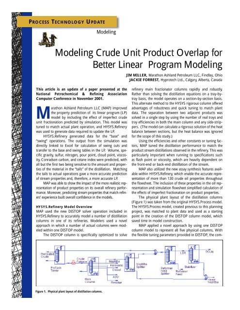
Figure 1. Physical plant layout of distillation columns.
JIM MILLER, Marathon Ashland Petroleum LLC, Findlay, Ohio
JACKIE FORREST, Hyprotech Ltd., Calgary, Alberta, Canada
refinery main fractionator columns rapidly and robustly.
Rather than solving the distillation equations on a tray-bytray
basis, the model operates on a section-by-section basis.
This alternate method to the HYSYS rigorous column offered
advantages of robustness and quick tuning to match plant
data. The separation between two adjacent products was
solved in a single step by using the number of real trays and
tray efficiencies in both the main column and any side-strippers.
(The model can calculate a rigorous solution of the heat
balance between sections, but the heat balance was ignored
for the scope of this study.)
Using the efficiencies and other constants or tuning factors,
MAP tuned the distillation performance to match the
product stream distillations observed in the refinery. This was
particularly important when running to specifications such
as flash point or viscosity, which are heavily dependent on
the front-end or back-end distillation of the stream.
MAP also utilized the new assay synthesis features available
within HYSYS.Refinery, which enable the accurate re p resentation
of more than 130 crude oil pro p e rties thro u g h o u t
the flowsheet. The inclusion of these pro p e rties in the oil re presentation
and simulation flowsheet simplified calculation of
the effects of imperfect fractionation on product pro p e rties.
The physical plant layout of the distillation columns
(Figure 1) was taken from the original HYSYS.Process model.
The HYSYS.Process model, created previous to this planning
project, was matched to plant data and used as a starting
point in the creation of the DISTOP column model, which
saved time in model construction.
MAP applied a novel approach by using one DISTOP
column model to represent all five physical columns. With
the flexible tuning parameters provided in DISTOP, the com-

pany was able to tune the model to accurately represent the
various product qualities and quantities to match plant data.
The model in HYSYS.Refinery uses a sub-flowsheet feat
u re. In the main flowsheet, the user sees the model as a type
of black box, only re p o rting the streams in and out of the unit.
The user can drill down to another level of detail by opening
the sub-flowsheet and studying the actual topology of the column
model. Figure 2 shows the DISTOP column model fro m
the main environment. Figure 3 depicts the more detailed re presentation
of the model in the sub-flowsheet enviro n m e n t .
In Figure 3, each side stripper, the separation trays above
its draw, and the pumparound above can be viewed as a separate
column. Each separate column gets its feed from the top
of another column and splits it into a bottoms product and a
mix of lighter products that is fed to another column.
By stacking enough of these columns together, MAP
could simulate a collection of columns as a single column.
Figure 2 shows, ironically, that after all the work to
include overlap instead of perfect separation, MAP used four
component splitters to calculate pure component yields for
butane and lighter products because the LP expects light-end
data in that format.
Plant Data Overview
The standard way of displaying distillation data is a cumulative
curve of percent distilled, with percent distilled on the xaxis
and temperature on the y-axis. This leads to S-shaped
curves typical for crudes and most products. A typical plot is
shown in Figure 4.
The distillation of the products and the crude also are displayed
on the same axis. Each S-shaped curve starts and ends
with a near- v e rtical segment re p resenting the product tails. The
horizontal distance between the beginning and ending segments
gives a measure of the total volume of the cut, while the
v e rtical distance gives a measure of the boiling range of the
material. Drawing this type of plot re q u i res the volumes of all
the products to arrange them on the horizontal axis.
The volume interchange between cuts (light material in
the heavier product, and the heavy material in the lighter
product) is difficult to see with this type of plot. This value
can be calculated by examining the area between the two
product curves, and it is related to how close the plot of a
product distillation comes to the plot of the crude.
Another way to look at the distillation data, shown in
Figure 5 (on page 26), is by plotting in incremental barrels of
crude and product vs. temperature instead of cumulative barrels.
In this case, the products will plot as bell-shaped curves.
The volume of each cut is the area under the curve. The overlap
range is where the curves cover the same temperature,
and the volume i n t e rchange is being the area under the curv e
in the overlap temperature range. With this plot, one can
examine the extent of overlap between products for the distillation
section.
Figure 5 illustrates the significant overlap of five different
products at 410 o F. Overlaps of diesel, kerosene, and
heavy naphtha are important because these products have
P R O C E S S T E C H N O LO GY U P D AT E
Figure 2.DISTOP column model from the main flowsheet in the HYSYS.Refinery model.
Figure 3.Sub-flowsheet representation of the model.
Figure 4. Typical display of distillation data.

P R O C E S S T E C H N O LO GY U P D AT E
Figure 5.Plot of distillation data using incremental, rather than cumulative, values for barrels of crude.
Figure 6. Plots of atmospheric gasoil (AGO) and residue streams demonstrate consideratable overlap.
varying specifications on properties that are strongly affected
by the heaviest components.
To focus attention, only the data for the atmospheric gas
oil (AGO) and residue streams are plotted in Figure 6. These
show that AGO and residue overlap by several hundred
degrees, and the residue initial boiling point (IBP) is almost
the same as the AGO IBP. This can be modeled with the flexible
tuning factors available in the DISTOP model. These
substantial overlaps are the driving force behind including
their effects in the LP model.
Modeling Product Overlap in the LP
Crude oil assay information systems generally give perfect
cuts. Users can adjust the calculation slightly to give some
overlap between adjacent cuts, but there is no
obvious correlation between the parameters
and the overlap in the plant. Also, there is no
way to make three or four products overlap.
When information from typical crude oil assay
systems is put into the LP program, the tails of
the distributions are effectively ignored. The
swing cut properties tend to be very near the
properties of the crude at the cutpoint. For
example, if the cutpoint is raised from 400ºF to
405ºF, the properties of the crude in the range
from 400ºF to 405ºF get averaged into the
properties of the lighter product and removed
from the properties of the heavier product.
By modeling the overlaps more carefully,
the properties of the swing cuts will affect the
product tails. A change in cutpoint from 400 ºF
to 405ºF will add some new material that boils
between 450ºF and 455ºF (or even higher) to
the lighter product. If the property is sensitive
to heavy ends (sulfur, cloud point), the more
representative model will supply better data to
the LP and result in better modeling of the
plant. Similar considerations apply to the light
tail, for which viscosity and flash point are sensitive
to light components.
Model Tuning
After configuration, the model must be tuned to
accurately re p resent the re f i n e ry products with
overlap. In principle, one should fit the model
results to plant data. For this study, the original
HY S Y S distillation results were used. The
HY S Y S model had been previously matched to
operations for a particular day. Using data that
come from a simulation introduces some
smoothing in the data being tuned to fit.
The true boiling point (TBP) curve of the
c rude feed in the HYSYS.Refinery model was comp
a red to the TBP curve in the HYSYS model to be
s u re it accurately re p resented the feed. The model
feed TBP should be compared to the plant feed
T B P, re g a rdless of whether the plant feed TBP is from laboratory
data on the actual feed or a back blend of the pro d u c t s .
The column model was tuned to give the same product
yields and distillations as the process model by adjusting the
separation efficiency and stripper efficiency factors for each
section. The front shape factor for the heavy naphtha was
also adjusted to give a slightly better fit. After the first tuning,
a second pass was used to fine-tune the results. In this
case, MAP chose the manual method because it gave results
quickly that matched the desired data within the acceptable
tolerances, but alternate methods are available to automate
the tuning.
F i g u re 7 shows the results for the kero s e n e
HYSYS.Refinery modeled product distillation curves and

Figure 7.Plots of modeled and actual data for kerosene show good agreement.
P R O C E S S T E C H N O LO GY U P D AT E
plots generated using actual data. Other products matched
within acceptable tolerances.
The DISTOP tuning factors are defined as follows:
• Section efficiency—Average efficiency of trays in
product section above the stripper draw. It affects
quality of fractionation or volume interc h a n g e
between products.
• Stripper efficiency—Average efficiency of trays in
product stripper. It affects stripout of light-boiling
material in product and temperature drops across
the stripper.
• Front and back shape factors—Front shape factor
affects the 1% and 5% points of the product. Back
shape factor affects the 95% and 99% points of the
next lighter product.
Most products were easily tuned with the section and
stripper efficiency. Only the heavy naphtha stream needed
fine-tuning with the front shape factor.
Crude Assay Preparation
Using HYSYS.Refinery Model
MAP uses five main crude feeds at the site where processing was
being modeled. The data to re p resent each of these crude oils
p reviously existed in Excel. Links from HYSYS.Refinery to Excel
w e re created to automate the loading of the crude oil assays.
The columns were first modeled at base conditions. All
of the product properties and yields were collected for the
base-case conditions. Next, one by one, each cutpoint was
adjusted by the maximum variation allowed in the plant,
which also should be the amount modeled in the LP. For each
of the new cutpoints, the resulting product properties and
yields were recorded.
Swing cut properties were calculated in the Excel environment.
Two HYSYS.Refinery runs produced property information
for each product stream, both including and excluding
the swing material. The properties for each swing cut
were calculated by difference. In fact, most properties were
calculated twice by diff e rence, once
from changes to the lighter product and
a second time from changes to the
heavier product. There were some
exceptions; for example, Conradson
carbon is not calculated for light
streams. In the case of Conradson carbon,
the swing stream property is calculated
only from the difference in the
heavy stream.
HYSYS.Refinery supports a long
and growing list of properties; however,
in this study, only specific gravity, sulfur,
nitrogen, pour point, cloud point,
v i s c o s i t y, Conradson carbon, and
cetane index were examined.
LP Results
Two sets of crude assays were prepared,
with the original set based on the original laboratory
data cut into nominal products. The swing streams were
modeled with no overlap. This model was referred to as
“square cuts.”
A second set of assays were based on the
H Y S Y S . R e f i n e ry model using overlapping products and
swing stream properties calculated by difference. This was
referred to as “overlapping cuts.”
For any given crude, the assay model has different yields
and properties. The products in the overlap case have wider
boiling ranges than the square case because the overlap case
includes the product tails. Including the tails has a non-linear
effect on product properties. Some properties, such as
viscosity, are inherently non-linear. They are much more sensitive
to a small amount of less viscous material than an equal
amount of very viscous material, but even properties that follow
a material balance have non-linear effects. For example,
if both heavy and light tails are added to a product, the sulfur
in the product will go up because the sulfur is not distributed
evenly or linearly. A plot of sulfur vs. boiling point
for a crude isn’t flat or even an upward sloping straight line.
It is a curve that slopes upward and gets steeper as the temperature
increases.
For most products, the heavy tails will dominate the
light tails, and the properties will look worse in the overlap
case than they do in the square case, with residue as the one
exception. There is no material to add as a heavy tail to the
resid, but there is a light tail to add so the resid sulfur is lower
in the overlap case than the square case.
Table 1 (on page 30) shows the sulfur content of the
product and swing streams for the two crudes used in this
study. The sulfur predictions for the square and overlapped
cases are shown for each crude. Note that the residue has a
lower sulfur content in the overlapped case than in the
square cut residue, but the lighter streams have more sulfur.
The same data also are represented graphically in Figure 8.
The resulting two sets of assays were used with the

P R O C E S S T E C H N O LO GY U P D AT E
TABLE 1. SULFUR CONTENT IN PRODUCT AND SWING STREAMS FOR TWO CRUDE OILS
Cut Name Naphthas & Kerosene Kerosene Diesel Diesel AGO Residue
Heavy Crude
lighter swing swing
S square cut (wt%) 0.004 0.005 0.013 0.036 0.090 0.174 0.509
S overlapped (wt%) 0.004 0.006 0.042 0.068 0.120 0.206 0.487
Yield (%) 36.9 2.5 6.7 11.9 1.7 8.9 31.4
Light Crude
S square cut (wt%) 0.005 0.009 0.013 0.030 0.050 0.085 0.311
S overlapped (wt%) 0.005 0.011 0.028 0.040 0.078 0.133 0.295
Yield (%) 39.9 3.2 7 9.8 1.2 7.1 31.8
Figure 8.Overlapped and square-case product sulfur for heavy and light crude.
Figure 9.Simplified refinery LP model for a system with two crude units.
“standard” LP model in one of Marathon Ashland Petroleum’s
refineries. This refinery has two crude units. The crude mix
to the first unit was fixed for all cases. The second unit was
required to take small, fixed amounts of other crudes and, in
addition, could choose between the heavy and light crude up
to plant capacity limits and maximum purchase limits. Most
of the products have minimum sales re q u i rements and many
also have maximum sales limits. The effect of these limits was
to force extra capacity into gasolines, low-sulfur diesel, highsulfur
diesel, and an intermediate stream that is sold to another
re f i n e ry.
At the re f i n e ry, both AGO and the residue products feed
to the cat cracker. The diesel swing stream can go to the diesel
s t ream to make distillate products or to the cat cracker.
For all the examples, the LP consistently sent the diesel
swing to the AGO and thus to the cat cracker. All of the other
swing streams stayed with their base-case arrangement, so
the comparisons are simplified to what the LP does with the
potential crude slate. Figure 9 depicts the simplified refinery
LP model.
S q u a re cut re s u l t s : Even though the heavier, more -
expensive crude has more sulfur than the lighter crude, the LP
found it more valuable because it provided more feed to the
cat cracker and thus more gasoline products. The LP used as
much heavy crude as it could up to a maximum purc h a s e
limit. It also used some of the lighter crude. Except for blending
ethanol or other additives, the LP didn’t run up against
any product quality limits. It was able to blend kerosene and
diesel (mostly from heavy crude) to make low-sulfur fuel oil
well within the sulfur limit. This was because the square cut
diesel sulfur was 0.036 wt% and the square kerosene sulfur
was 0.013 wt%. As might be expected, when blended, these
p roducts were under the 0.045 wt% sulfur limit.
Overlap cut results: In the overlap case, the LP prefers
the light crude to the heavy one. If it uses the heavy crude, it
runs into a constraint when it tries to blend diesel (0.068
wt% sulfur) and kerosene (0.042 wt% sulfur) from the second
crude unit. The low-sulfur fuel oil product has a maximum
sulfur content of 0.045 wt%. To make the 0.045 wt%
limit, it has to use the light crude, with its 0.028 wt% and
0.040 wt% sulfur contents for kerosene and diesel, respectively.
The light crude, although cheaper, makes less cat feed,
which requires the purchase of more outside cat feed and
therefore results in somewhat less overall profit.
Hybrid case: Running a third case further compares the

P R O C E S S T E C H N O LO GY U P D AT E
TABLE 2.DIFFERENCES BETWEEN THE SQUARE-CUT, OVERLAP, AND HYBRID CASES ON KEY MEASURES.
I n c remental change vs. square-cut base case bbl/day I n c remental change vs. square base case bbl/day
overlap hybrid overlap hybrid
Refinery inputs Low-sulfur diesel
Light crude 20,622 0 First kerosene 0 2,522
Heavy crude -24,721 0 Second kerosene -284 -2,522
Other crude 0 0 Second diesel -1055 -5,793
Purchased gasoil 1,965 0 Total -1339 -5,793
Other material -124 -4
Total -2,259 -4
Refinery outputs Hi-sulfur diesel
Gasoline & jet fuel -228 -212 Intermediate 0 4,797
Low-sulfur diesel -1,339 -5,793 Second diesel 0 5,793
Hi-sulfur diesel 0 10,590 Total 0 10,590
Intermediate 195 -4,649
Other material and FOE -1,106 1
Total -2,478 -63
two approaches. The crude slate picked from the square cut
case was run with the overlap properties. Essentially, this
modeled what is done today. Refiners choose their crude slate
based on square cut crude assays and run them through a
plant where there are overlaps. If one tried to make exactly
the same product slate as the square cut case, it would violate
p roduct specifications. The product rates were left
to float.
As expected, the LP downgraded some of the low-sulfur
diesel oil into high-sulfur diesel oil, and brought in some
k e rosene from the first crude unit. The LP revised the amounts
of various gasolines to free up some blending stock. The net
p rofit was a little lower than the overlap case. The financial
penalty could have been larger or smaller depending on the
low-high sulfur price diff e rential. The logistical problem of
suddenly having to find tankage, pipeline space, or a customer
for the high-sulfur fuel oil (and the loss of confidence in the
LP) was probably more important than the loss of pro f i t .
D i ff e rences between the cases for the more import a n t
p u rchases, sales, and intermediate streams are shown in Ta b l e
2. The low-sulfur diesel was 0.030 wt% in the square cut case
and at the limit of 0.045 wt% in both the overlapped and
hybrid cases. The values shown in Table 2 are the total incremental
barrels per day of change from the original square run.
The crudes for the first crude unit and the “other crudes”
for the second unit still have square cut properties. Changing
them to the overlapped properties creates greater differences
between the square and overlapped cases. For the hybrid
case, it results in even more downgrading of low-sulfur diesel
to high-sulfur diesel because the first unit’s kerosene will also
have higher sulfur.
In summary, the overlap between products can be modeled
and tuned to actual results. Modeling the overlap leads to diff e rent
physical pro p e rties for the products and swing streams. Wi t h
d i ff e rent pro p e rties, the LP will give significantly diff e rent re s u l t s .
The new model is more realistic and more easily related to
plant operation. HYSYS.Refinery, with its extensive list of accurate
re f i n e ry pro p e rties and ability to link to Excel, allowed this
p roject to be completed with accuracy and speed. ●
ABOUT THE AUTHORS
James H. Miller (Jim) B.S. Chemical
Engineering, 1971, Case Institute of Technology;
M.S. 1975 Ph.D. 1978, Case Western Reserve
University. He joined Marathon Oil Company in
1977 and worked at a number of positions
including nine and a half years in Aberdeen, Scotland. His
work includes steady state simulations, dynamic simulations
(training simulators), computer control and data acquisition,
hook-up and commissioning. After several corporate reorganizations
he is now with the Engineering and Analytical
Services Department (in Findlay, Ohio) which is part of
Marathon Ashland Petroleum LLC.
Jackie Forrest is the HYSYS.Refinery Product
Manager for Hyprotech. She works out of the
Calgary office. Her responsibilities include coordinating
marketing and development aspects
associated with HYSYS.Refinery, including development,
advertising, and development of technical and marketing
material. Ms. Forrest’s past work experience includes
both refinery operation and engineering design. Jackie graduated
from the University of Calgary with a bachelor of science
in chemical engineering.