LP Modeling - Past, Present and Future

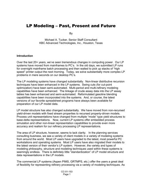
Introduction
LP Modeling – Past, Present and Future
By
Michael A. Tucker, Senior Staff Consultant
KBC Advanced Technologies, Inc., Houston, Texas
Over the last 20+ years, we’ve seen tremendous changes in computing power. Our LP
systems have moved from mainframes to PC’s. In the old days, we submitted LP runs
for overnight mainframe batch processing and then waited to pick up stacks of “high
speed” printer output the next morning. Today, we solve substantially more complex LP
problems in mere seconds on our desktop PC’s.
The LP modeling systems have changed substantially. Non-linear distributive recursion
techniques have been enhanced in the LP systems. Swing cuts (for cut-point
optimization) have been semi-automated. Multi-period and multi-refinery modeling
capabilities have been enhanced. The linkage of crude assay data into the LP assay
tables has been enhanced and semi-automated. Reformulated gasoline blending
capabilities have been incorporated into the systems. And, or course, the latest
versions of our favorite spreadsheet programs have always been available for
preparation of our LP model data.
LP model structure has also changed substantially. We have moved from non-recursed
yield-driven models with fixed stream properties to recursed property-driven models.
Process unit representations have changed from multiple “mode” type yield structures to
base-delta representations. Now, current LP systems offer embedded process
simulation and other non-linear representation capabilities to provide even more
accuracy and realism for our refinery processing LP representations.
The area of LP structure, however, seems to lack clarity. In the planning services
consulting business, we see a variety of client models in a variety of modeling systems
from around the world. Most LP users have upgraded to the latest, most powerful PC
workstations and operating systems. Most LP users have also migrated their models to
the latest version of their vendor’s LP system. However, the variety and types of
modeling philosophy, structure and modeling techniques used within these systems is
seemingly endless. There is definitely little “standardization” of LP model structure and
data representations in the LP models.
The commercial LP systems (Aspen PIMS, GRTMPS, etc.) offer the users a great deal
of flexibility for representing refinery processing via a variety of modeling techniques. As
CC-01-153
Page 1

a result, individual refinery LP model developers have used a variety of methods and
structure to represent their process unit submodels including: Multiple modes, basedelta
modeling, embedded simulation, pooling and distributive recursion. All of these
techniques have been applied to varying degrees in various models.
So, the question is: What’s is the best LP modeling method? Why?
In this paper, we discuss the trends and industry practices in LP refinery modeling.
What has changed in LP modeling and why has it changed? What are the common
modeling techniques, structure and data generating techniques that are being used
today? Where are we headed with modeling structure?
Hopefully, this paper will stimulate thinking about your refinery LP model. How does
your model structure and data compare with industry best practices? Should you
consider upgrading your LP model? What are the possible benefits? What are the
risks?
The goal is clear – what refiners want and need are LP planning models that accurately
represent the true capabilities and limitations of their refining facilities. We want the LP
model to give us sound advise about crude selection, process optimization, oil
movements, product blending and product optimization.
What isn’t always clear is what are the best modeling technologies and techniques to
achieve superior accuracy from the model? Also, what is the appropriate degree of
accuracy considering the trade-offs between the desire for simplicity, ease of use, and
the drive for accuracy?
Past LP Modeling
Going back a number of years (15 to 20), we had what I’ll call the Pre-Recursion type
models. These models had no stream pooling and no recursion. The crude unit models
were presented by a series of yield structures for each crude. The characteristics were:
• Each cutting scheme (max naphtha, max kerosene, etc.) had a separate yield
structure (mode) for each crude.
• The major side-cuts from each crude (and from certain cuts from each cutting
scheme) were unique streams, with unique names and unique (fixed) qualities.
• Generally, the crude assay table data was generated by a crude assay system
(containing a library of crude oils). Yields and properties from the assay system
were generally those predicted from laboratory TBP distillations. In many cases,
the systems were automated to generate the LP crude assay tables in the LP
assay table format.
CC-01-153
Page 2

The downstream process unit sub-models were also represented by a series of multiple
yield structures. The characteristics of the process unit sub-models were:
• Each feed to a downstream process unit was from a side-cut from a particular
crude.
• Each process unit feed has one or more yield structures (modes) representing
the processing of each unique feed under specific operating conditions e.g. a
particular reactor temperature.
• The products from each mode had fixed qualities. Frequently, each feed/mode
combination would produce streams with different fixed qualities.
• The yields were typically generated using simulation models. Each side-cut from
each crude was processed through the simulator at a particular operating
conditions (e.g. severity) to produce a unique set of yields and product properties
for the feedstock. In many cases, the simulators were automated to generate
the necessary yield structures for the LP model.
In our efforts to further differentiate one crude from another, we frequently generated
literally hundreds of yield structures for process unit sub-model to represent each
possible crude side-cut at multiple operating conditions and multiple cutting schemes.
Frequently, the process unit might be structured to produce anywhere from 4 to 20+
versions of each product stream (each with unique qualities associated with a particular
crude and/or cutting scheme).
Models of this type tended to have the following overall characteristics:
• There were generally 3 to 10 times as many individual streams in the model as
there were streams in the “real” refinery.
• There were generally 10 to 20 times as many final product blending options as
there were actual component blending options available in the “real” refinery.
Distributive Recursion Technique
During a Chevron LP training class at El Segundo, California in 1977, Bill Hart, a senior
mathematician from Haverly Systems, was working with Don White, a senior LP
modeler from Chevron. Don’s complaint was that these types of multiple yield and
mode type LP models tended to over-optimize the processing and blending of individual
crude and their associated side-cuts throughout the refinery. The model frequently
overstated the value difference between individual crudes. Don wanted a better way.
During that class, Bill Hart developed the mathematics for the recursion technique that
became known as Distributive Recursion (DR). Up to that time, some attempts had
been made to use a simple recursion technique. The Distributive Recursion technique
CC-01-153
Page 3

added the critical linkage between upstream changes in pool qualities to the quality
changes in the downstream destinations. Early versions of the DR technique were
slow and difficult to work with. Over the years since then, the technique has become
faster, better, and more reliable. The technique is increasingly popular and is now
widely accepted in the LP modeling systems and refinery models.
Current LP Modeling Practices
As mentioned earlier, there is an infinite variety of modeling techniques currently being
used. However, we can, at least, categorize and discuss current modeling practices in
the various areas of the LP model structure.
Crude Distillation Swing Cuts
Swing cuts are increasing used in LP assay tables to represent the refinery’s flexibility
to alter cut-points for optimization of side-cut yields and properties. When used, swing
cuts have generally replaced the older multiple “mode” type of yields structures. The
Aspen PIMS system, for instance, has provided a Type 4 swing cut in their CRDCUTS
table. The system will then automatically generate the necessary structure for blending
the swing cut up and down. Swing cuts are frequently used for Naphtha/Kerosene,
Kerosene/Diesel cuts and for Gasoil/Bottoms cuts as well as others. A majority of LP
models now employ swing cut architecture in at least some of the crude distillation side-
cuts. In general, the swing cuts are also used along with side-cut property recursion
techniques such that main side-cut yields and properties are impacted by the swing cut
blending.
Crude Assay Recursed Properties
Most crude assay tables now include recursed properties for the various side-cuts.
Typically, the side-cuts in the model now match the physical side-cuts from the “real”
refinery, with the exception of the swing cuts. The individual side-cuts generally have
anywhere from 3 or 4 recursed properties to over 20. The average number of recursed
properties in most models is about 7 to 10. The side-cut recursed properties are not
just used for product blending. The properties are now frequently used as product yield
and property drivers in downstream process units sub-models (e.g. % Naphthenes and
% Aromatics for Reformer sub-models).
Commercial Distillation Properties
LP crude assay data is frequently generated by using one or more of the vendor crude
assay libraries in conjunction with a commercial crude assay system. The assay data
from these libraries is based on laboratory distillation results. In the past, most LP’s
included these laboratory predicted properties, rather than commercial unit properties.
Increasingly, LP modelers are interested in getting the commercial unit distillation
results into the LP. Right now, there are three main techniques that are in common use:
CC-01-153
Page 4

1. Some modelers “offset” the laboratory properties in the LP model to more
accurately match the commercial results. This works reasonably well in those
situations where the crude slate is relatively stable.
2. In recent years, the vendor assay systems have added features designed to
allow a degree of side-cut overlap with associated property predictions. The
systems require the user to supply the parameters for the column tuning. These
parameters have been used with varying degrees of success.
3. Those refiners who maintain a tuned column simulation model (e.g. KBC
Petrofine DISTOP) generally use this column simulation along with an assay
library and system to generate the yields and properties for the LP assay table.
With this system, each of the library crudes is processed through the column
simulation to then predict the yields and properties for the side-cuts based on
the tuned column simulator. Multiple runs of the simulator are required to backcalculate
the properties of the swing cuts used in the LP model. Systems are
now becoming available to automate the multiple simulator runs and the back
calculation processes.
In recent years, the LP systems have added the capability to use multiple assay tables.
Hence, it is now convenient to provide customized and tuned yields and properties for
each of the refinery’s physical and/or logical distillation column operations.
Base-Delta Process Unit Sub-Models
Concurrent with the development and implementation of DR is the use of base-delta
modeling techniques for major process unit sub-models. The base-delta modeling
technique has the following characteristics:
1. A single base yield structure provides the yields and product properties
associated with a typical quality feed at normal operation conditions. This yield
structure is customized and tuned to the particular refinery process unit. In some
variations of this technique, multiple base yields are provided at alternative
severities of operation. In most cases, the base yield structure is generated
from a single run of a tuned simulator for the particular process unit.
2. Feed property drivers are used to provide shifts (or correctors) for changes in
feed properties relative to the base feed quality. These shift correctors represent
the linear change in yields (and product properties) as a function of changes in
feed properties. These shift correctors are generally calculated by the use of the
process simulators. DR techniques are used to provide the necessary feed
properties from the various upstream sources and feed pools.
There are two common techniques used to generate these correctors:
CC-01-153
Page 5

a. The perturbation technique changes each feed property independently (up
and down) and then calculates the linear shift from the perturbation cases.
b. A multi-variable linear regression technique is used to calculate the linear
shift correctors based on the regressed results for product yields and
properties from a large number of feed property scenarios when run
through the simulator.
3. Operating variable drivers are provided to shift yields (and product properties) off
the base for changes in operating conditions (typically severity). Again, the
process simulators are generally used to generate the delta shifts for these
operating conditions.
4. DR techniques are frequently used to recurse on key product properties. The
base, feed property drivers, and operating variable shifts all contain coefficients
that calculate the appropriate recursed product properties. Process unit product
stream properties are either variable (recursed) or fixed. In general, if the
product property remains relatively constant regardless of the feed and/or
operating shifts, then the property may be fixed. Otherwise, the property should
be recursed. The use of product stream recursion has eliminated the need for
multiple versions of the same stream (as used in pre-recursion models). Now,
the streams in the LP model (represented by pools with recursed properties)
more closely match the streams in the “real” refinery.
5. Many of the major process unit sub-models now use swing cuts for key cutpoint
optimization representations. Multiple runs of the process simulators are
generally used to back-calculate the yields and properties for the swing cuts used
in the process sub-models.
6. Most base-delta models now use multiple capacity constraints. Many of the older
models simply had one (maximum throughput) constraint. With base-delta
models using severity shifts, it is now appropriate to include several other
capacity constraints associated with operating constraints and variables e.g.
maximum air blower limits on an FCC unit or main fractionator side-cut draw
limits.
Local Optimal Problems
Most of the current LP models have some degree of pooling and property recursion.
The DR technique requires initial guesses for pool qualities and fractional distributions
of the pools to downstream destinations. As with any non-linear technique, there will be
a risk of local optimal solutions i.e. a solution that does not represent the highest
possible objective function. In all local optimal cases, the initial guesses and the
subsequent recursion calculations lead to a solution that is not the global optimum.
CC-01-153
Page 6

For models that contain a moderate (or higher) degree of recursion, there are only two
situations:
1. The model users have experienced local optimal problems and they know they
exist.
2. The model users don’t know they have local optimal problems (however, they do
exist but they have not yet been discovered by accident or testing).
We’ve found that almost every model that contains a moderate (or higher) level of
recursion experiences local optimal problems (some more than others). This is a
serious problem that can lead to a lack of confidence in the model results. Local
optimal problems in recursed LP’s cannot be completely eliminated but they can be
managed. It takes a combination of:
1. Good model structure that avoids unnecessary recursion and things like
cascading recursed pools and large numbers of downstream destinations for
recursed pools.
2. Attention to correctly setting the initial guesses and the recursion control
parameters. The system default recursion control parameters are not always the
best settings.
3. Testing for local optimal conditions and then analyzing and understanding the
conditions under which they occur and correcting those conditions.
Blending
In the blending area, current LP models contain significantly more property
specifications than in the past. The sophistication required for the blending equations is
increasing – as evidenced by reformulated gasoline. Increasingly, the blend
components in the model are nearly the same as those that exist in the “real” refinery
(via recursed pools) and the component properties are frequently linked all the way
back (via distributive recursion) to the properties of the side-cuts in the crude assay
tables.
Multi-Refinery and Multi-Period Modeling
There is an increasing use of multi-period and multi-refinery modeling by the user
community. Mainly, this trend is the result of faster computers and enhanced features in
the LP modeling systems for handling the parameters and input associated with multiperiod
and multi-refinery. (It’s also the results of all of those mergers and acquisitions in
the industry).
There is one caution, however, in that recursed models tend to be unstable (i.e. local
optimal and/or non-converged) when attempting to use both multi-period and multi-
CC-01-153
Page 7

efinery in the same case. Also, there are limitations on the use of multi-refinery. In
general, no more than about 3 refineries should be attempted with recursed LP multirefinery
models. Large recursed multi-refinery models tend to be unstable as
represented in the following graph.
Recursed Pools
600
500
400
300
200
100
1000 3000 5000 7000 9000
Model Maintenance
1
2
Stable
Matrix Rows
3 Refineries
Unstable
This paper is mainly about LP model structure. However, there are some important
points to be made about generating the LP data and maintaining the LP model. In the
past, we occasionally (every few months) compared the actual plant process data with
the LP predicted yields. We looked at combinations of test run results, historical
process data, and yield accounting data when updating LP models and sub-models. LP
sub-models were not frequently updated (maybe once every couple of years) and the
methodology for updating the LP sub-model was not very well defined.
Currently, there are two main best practice methods for monitoring LP performance and
maintaining and updating LP models. First, an overall refinery backcasting process may
be used to identify overall model weaknesses (e.g. refinery gain higher than actual) and
profit opportunities. Backcasting is comparing a previous month’s actual results against
the plan and against an LP-actual case (where the LP case attempts to match actual
results). Many refineries conduct backcasting on a regular basis (at least several times
each year). LP maintenance activities are frequently based on the backcast results.
The second major activity is for process engineers to monitor their process units on a
weekly or bi-weekly basis. Lab samples, along with plant historian data are used to
compare the actual process unit results (yields and properties) against the LP predicted
CC-01-153
Page 8

esults for the same snapshot period. Process engineers and planners monitor and
compare the actual against the LP predicted and decide if the LP sub-model needs
updating. In most cases, a process simulator model may be re-calibrated and used to
generate the LP base and delta correctors on an as-needed basis. With this technique,
process unit sub-models may be updated as frequently as several times a year using
plant data and tuned simulator models.
Future LP Developments
The LP system vendors are now touting the virtues of the latest major LP system
enhancement: simulator interfaces. With the simulator interface, the LP system may be
directed to an outside application during each recursion pass. This outside application
may be as simple as a single non-linear equation or as complex as several large
complex process simulation models.
The concept is that model coefficients that were previously static (i.e. unchanged during
recursion) now become dynamic (changing after each recursion pass). For example,
the feed % naphthene and % aromatics linear yield shift correctors commonly used in
reformer LP models are generally based on particular feed qualities and severities.
These linear correctors are calculated externally during the model development and
then built into the model. These yield correctors are not updated during recursion. The
LP model predicted yields become less accurate if the LP optimized feed deviates
significantly from the base feed quality assumptions.
With the simulator interface option, these linear feed property correctors may now be
calculated and updated during each recursion pass, and then used for the next
optimization pass. As the model optimizes the feed quality and severity after each
pass, the naphthene and aromatics correctors are then adjusted to match the last pass
results. This improves the accuracy since the final converged solution of the LP more
closely matches the results of the simulation prediction.
However, the risk of a local optimal solution may increase, since more and more
coefficients are recursed and the initial starting assumptions for feed quality and
severity become increasingly important as they may influence the final converged
solution.
A number of refiners have successfully developed useful and reliable applications for
the simulator interface. There are a number a relatively simple non-linear applications
being used where previously unsolvable non-linear relationships have now been
handled with the simulator interface. For instance, in one application, we needed to
control the percent of a particular feed to a process unit. In this particular case, the
percent was an unknown and the process unit feedrate was also an unknown. This was
previously unsolvable with DR. However, with the simulator interface, it was now
possible to externally calculate the correct percent (based on the first optimized
solution) and then update the percent following each recursion pass.
CC-01-153
Page 9

Larger simulator interface applications have also been tested and developed using, for
example, embedded reformer simulator models, FCC simulation models and, most
recently, crude unit simulation with cutpoint shifts and cutpoint optimization (replacing
swing cuts).
Will this be the future of LP models? Perhaps. There are a number of issues to be
solved: slow calculations, local optimal problems, complexity of data input, complexity
of model output, etc. History would suggest that these problems can and will be
solved. Also, the general trend over the years has been towards the use of additional
non-linear techniques (mostly recursion) driven by the refiners desire for improved
accuracy. Certainly, the simulator interface is a logical step in that same direction of
improved accuracy.
Conclusion
LP systems accommodate a variety of modeling technique, structure and philosophies.
Your current LP model structure is usually a complex function of the particular refining
configuration, the LP system, economic drivers, logistical operational constraints,
process unit simulation model availability, initial and legacy model structure, LP
maintenance, backcasting analysis, and past and current LP modeler knowledge and
experience.
The industry, in general, is trending towards models that use pooling and distributive
recursion techniques to provide more realistic and accurate representations of the
refinery in the LP system.
What are the benefits of LP improvements? This has always been a difficult area to
address. The KOA paper from last year’s conference suggests one method. Intuitively,
most refining companies recognize the value of improved accuracy in their refinery LP
representations and the technology has been moving in that direction over the years.
We see improved LP accuracy in two areas: absolute accuracy and incremental
accuracy. Improved absolute accuracy is achieved by frequent tuning and updating of
the LP base yields and properties. Improved incremental accuracy is achieved through
superior LP modeling structure that provides the correct effects for incremental changes
throughout the refinery – from crude to products. Improvements in both of these areas
may lead to millions of dollars of annual profit improvement resulting from plans and
operating decisions that better utilize the refining asset.
The following table contains a checklist of best practice LP modeling features and
structure (discussed above) that should be considered and evaluated for your particular
modeling circumstances.
CC-01-153
Page 10

Every refinery LP model situation is unique. Some of these features may not be best
suited for your particular circumstances. However, in general, if your model structure
lacks these features, you may wish to consider the merits of an LP upgrade.
LP Model Structure Checklist
Streams in the LP model generally match streams that exist in the refinery �
LP Model uses pooling with recursion on key properties of the pools �
Crude unit side-cut properties are based on commercial distillation
�
performance on individual crude units. Tuned distillation simulation is used
to generate data for the LP assay tables.
Swing cuts are used in crude units and downstream process unit LP sub- �
models to represent cut-point optimization capabilities
Base-delta LP structure for major downstream process unit representations �
Tuned simulators used to generate base and delta yield and properties for �
major downstream process unit LP models
Process unit LP models include both key feed property drivers and key �
operating variable shifts
Multiple, realistic process unit constraints �
Local optimal risk minimized with appropriate structure and recursion �
control settings
Testing for and correcting local optimal conditions �
Frequent backcasting for LP model audit and opportunity evaluation �
Process unit routine monitoring, evaluation and LP process model updating
based on tuned simulation models
�
About the Author
Michael A. Tucker is a Senior Staff Consultant at KBC Advanced Technologies, Inc.
based in Houston, Texas. Mike is currently responsible for providing Planning Services
to worldwide refinery clients, including the management of LP upgrade projects. Mike
has 31 years of oil industry experience working, supporting and consulting on LP
planning for Chevron Corporation, Caltex Petroleum Corporation and KBC Advanced
Technologies. Mike holds a B.S. in Chemical Engineering from Purdue University.
Petrofine ® is a registered trademark of KBC Process Technologies, Ltd. Aspen PIMS is a registered
trademark of Aspen Technology. GRTMPS is a registered trademark of Haverly Systems, Inc.
CC-01-153
Page 11