A FAST AND ROBUST FRAMEWORK FOR IMAGE FUSION AND ...
A FAST AND ROBUST FRAMEWORK FOR IMAGE FUSION AND ...
A FAST AND ROBUST FRAMEWORK FOR IMAGE FUSION AND ...

Create successful ePaper yourself
Turn your PDF publications into a flip-book with our unique Google optimized e-Paper software.
UNIVERSITY OF CALI<strong>FOR</strong>NIA<br />
SANTA CRUZ<br />
A <strong>FAST</strong> <strong>AND</strong> <strong>ROBUST</strong> <strong>FRAMEWORK</strong> <strong>FOR</strong> <strong>IMAGE</strong> <strong>FUSION</strong> <strong>AND</strong><br />
ENHANCEMENT<br />
A dissertation submitted in partial satisfaction of the<br />
requirements for the degree of<br />
Lisa C. Sloan<br />
Vice Provost and Dean of Graduate Studies<br />
DOCTOR OF PHILOSOPHY<br />
in<br />
ELECTRICAL ENGINEERING<br />
by<br />
Sina Farsiu<br />
December 2005<br />
The Dissertation of Sina Farsiu<br />
is approved:<br />
Professor Peyman Milanfar, Chair<br />
Professor Ali Shakouri<br />
Professor Michael Elad<br />
Doctor Julian Christou
Copyright c○ by<br />
Sina Farsiu<br />
2005
Contents<br />
List of Figures vi<br />
List of Tables xiii<br />
Abstract xiv<br />
Acknowledgements xvi<br />
Dedication xviii<br />
Chapter 1 Introduction 1<br />
1.1 Super-Resolution as an Inverse Problem .................... 5<br />
1.2 Organization of this thesis . ........................... 9<br />
Chapter 2 Robust Multi-Frame Super-resolution of Grayscale Images 11<br />
2.1 Introduction .................................... 11<br />
2.2 Robust Super-Resolution . ........................... 16<br />
2.2.1 Robust Estimation . ........................... 16<br />
2.2.2 Robust Data Fusion ........................... 18<br />
2.2.3 Robust Regularization .......................... 23<br />
2.2.4 Robust Super-Resolution Implementation ................ 28<br />
2.2.5 Fast Robust Super-Resolution Formulation ............... 33<br />
2.3 Experiments . . . ................................ 34<br />
2.4 Summary and Discussion . ........................... 38<br />
Chapter 3 Multi-Frame Demosaicing and Color Super-Resolution 46<br />
3.1 Introduction .................................... 46<br />
3.2 An overview of super-resolution and demosaicing problems .......... 47<br />
3.2.1 Super-Resolution . . ........................... 47<br />
3.2.2 Demosaicing ............................... 48<br />
3.2.3 Merging super-resolution and demosaicing into one process . . .... 51<br />
3.3 Mathematical Model and Solution Outline .................... 54<br />
3.3.1 Mathematical Model of the Imaging System ............... 54<br />
iii
3.4 Multi-Frame Demosaicing . ........................... 57<br />
3.4.1 Data Fidelity Penalty Term . . . ..................... 58<br />
3.4.2 Spatial Luminance Penalty Term .................... 59<br />
3.4.3 Spatial Chrominance Penalty Term . . . ................ 60<br />
3.4.4 Inter-Color Dependencies Penalty Term . ................ 60<br />
3.4.5 Overall Cost Function .......................... 61<br />
3.5 Related Methods . ................................ 63<br />
3.6 Experiments . . . ................................ 64<br />
3.7 Summary and Discussion . . ........................... 69<br />
Chapter 4 Dynamic Super-Resolution 83<br />
4.1 Introduction .................................... 83<br />
4.2 Dynamic Data Fusion . . . ........................... 85<br />
4.2.1 Recursive Model . . ........................... 85<br />
4.2.2 Forward Data Fusion Method . ..................... 88<br />
4.2.3 Smoothing Method . ........................... 94<br />
4.3 Simultaneous Deblurring and Interpolation of Monochromatic Image Sequences 98<br />
4.4 Demosaicing and Deblurring of Color (Filtered) Image Sequences . . . .... 99<br />
4.5 Experiments . . . ................................ 101<br />
4.6 Summary and Discussion . ........................... 109<br />
Chapter 5 Constrained, Globally Optimal Multi-Frame Motion Estimation 110<br />
5.1 Introduction .................................... 110<br />
5.2 Constrained Motion Estimation .......................... 112<br />
5.3 Precise Estimation of Translational Motion with Constraints .......... 115<br />
5.3.1 Optimal Constrained Multi-Frame Registration . . . .......... 115<br />
5.3.2 Two-Step Projective Multi-Frame Registration . . . .......... 116<br />
5.3.3 Robust Multi-Frame Registration .................... 118<br />
5.4 Experiments . . . ................................ 118<br />
5.5 Summary and Discussion . ........................... 120<br />
Chapter 6 Conclusion and Future work 123<br />
6.1 Contributions . . . ................................ 123<br />
6.2 Future Work . . . ................................ 126<br />
6.3 Closing ...................................... 130<br />
Appendix A The Bilateral Filter 131<br />
Appendix B The Limitations and Improvement of the Zomet Method [1] 133<br />
Appendix C Noise Modeling Based on GLRT Test 136<br />
Appendix D Error Modeling Experiment 138<br />
Appendix E Derivation of the Inter-Color Dependencies Penalty Term 140<br />
iv
Appendix F Appendix: Affine Motion Constraints 142<br />
Bibliography 144<br />
v
List of Figures<br />
1.1 A block diagram representation of image formation and multi-frame image reconstruction<br />
in a typical digital imaging system. The forward model is a mathematical<br />
description of the image degradation process. The inverse problem<br />
addresses the issue of retrieving (or estimating) the original scene from the lowquality<br />
captured images. . . ........................... 2<br />
1.2 An illustrative example of the motion-based super-resolution problem. (a) A<br />
high-resolution image consisting of four pixels. (b)-(e) Low-resolution images<br />
consisting of only one pixel, each captured by subpixel motion of an imaginary<br />
camera. Assuming that the camera point spread function is known, and the<br />
graylevel of all bordering pixels is zero, the pixel values of the high-resolution<br />
image can be precisely estimated from the low-resolution images. . . . .... 3<br />
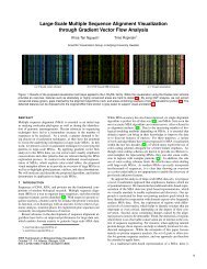
1.3 Super-resolution experiment on real world data. A set of 26 low quality images<br />
were fused resulting in a higher quality image. One captured image is shown in<br />
(a). The red square section of (a) is zoomed in (b). Super-resolved image in (c)<br />
is the high quality output image. ......................... 5<br />
2.1 Block diagram representation of (2.1), where X(x, y) is the continuous intensity<br />
distribution of the scene, V is the additive noise, and Y is the resulting<br />
discrete low-quality image. . ........................... 12<br />
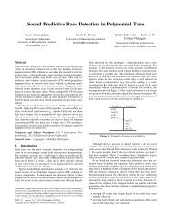
2.2 Simulation results of outlier effects on super-resolved images. The original<br />
high-resolution image of Lena in (a) was warped with translational motion and<br />
down-sampled resulting in four images such as (b). (c) is an image acquired<br />
with downsampling and zoom (affine motion). (d) Reconstruction of these four<br />
low-resolution images with least-squares approach. (e) One of four LR images<br />
acquired by adding salt and pepper noise to set of images in (b). (f) Reconstruction<br />
of images in (e) with least-squares approach. ................ 19<br />
vi
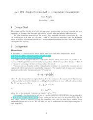
2.3 Effect of upsampling D T matrix on a 3 × 3 image and downsampling matrix D<br />
on the corresponding 9 × 9 upsampled image (resolution enhancement factor of<br />
three). In this figure, to give a better intuition the image vectors are reshaped<br />
as matrices. In this thesis, we assume that the blurring effects of the CCD are<br />
captured by the blur matrix H, and therefore the CCD downsampling process<br />
can be modeled by a simple periodic sampling of the high-resolution image.<br />
Hence, The corresponding upsampling process is implemented as a zero filling<br />
process. ...................................... 22<br />
2.4 a-e: Simulation results of denoising using different regularization methods. f:<br />
Error in gray-level value estimation of the pixel indicated by arrow in (a) versus<br />
the iteration number in Tikhonov (solid line), TV (dotted line), and Bilateral<br />
TV (broken line) denoising. . ........................... 27<br />
2.5 Simulation results of deblurring using different regularization methods. The<br />
Mean Square Error (MSE) of reconstructed image using Tikhonov regularization<br />
(c) was 313. The MSE of reconstructed image using BTV (d) was 215. . . 29<br />
2.6 Block diagram representation of (2.22), blocks Gk and Rm,l are defined in Figure<br />
2.7. ...................................... 31<br />
2.7 Extended Block diagram representation of Gk and Rm,l blocks in Figure 2.6. . 31<br />
2.8 Reconstruction of the outlier contaminated images in Figure 2.2. Non-robust<br />
reconstructed images in Figures 2.2(d) and 2.2(f) are repeated in (a) and (b),<br />
respectively for the sake of comparison. The images in (c)-(d) are the robust<br />
reconstructions of the same images that was used to produce Figures (a)-(b),<br />
using equation (2.22). Note the shadow around the hat in (a) and the salt and<br />
pepper noise in (b) have been greatly reduced in (c) and (d). .......... 32<br />
2.9 Controlled simulation experiment. Different resolution enhancement methods<br />
(r =4) are applied to the Figure (b). . ..................... 40<br />
2.9 Controlled simulation experiment. Different resolution enhancement methods<br />
(r =4) are applied to the Figure (b). . ..................... 41<br />
2.10 Results of different resolution enhancement methods (r =4) applied to Tank<br />
sequence. ..................................... 42<br />
2.11 Results of different resolution enhancement methods (r =4) applied to Adyoron<br />
test sequence. ................................ 43<br />
2.12 Results of different resolution enhancement methods (r = 3) applied to the<br />
Alpaca sequence. Outlier effects are apparent in the non-robust reconstruction<br />
methods. ...................................... 44<br />
2.12 Results of different resolution enhancement methods applied to the Alpaca sequence.<br />
Outlier effects are apparent in the non-robust reconstruction method<br />
(g). The shadow of the Alpaca is removed in the robust reconstruction methods<br />
of (h),(i), and (j). . ................................ 45<br />
vii
3.1 A high-resolution image (a) captured by a 3-CCD camera is down-sampled by a<br />
factor of four (b). In (c) the image in (a) is blurred by a Gaussian kernel before<br />
down-sampling by a factor of 4. The images in (a), (b), and (c) are color-filtered<br />
and then demosaiced by the method of [2]. The results are shown in (d), (e), (f),<br />
respectively. . . . ................................ 52<br />
3.2 Fusion of 7 Bayer pattern low-resolution images with relative translational motion<br />
(the figures in the left side of the accolade) results in a high-resolution<br />
image ( � Z) that does not follow Bayer pattern (the figure in the right side of<br />
the accolade). The symbol “?” represents the high-resolution pixel values that<br />
were undetermined (as a result of insufficient low-resolution frames) after the<br />
Shift-and-Add step (Shift-and-Add method is extensively discussed in Chapter 2). 53<br />
3.3 Block diagram representing the image formation model considered in this chapter,<br />
where X is the intensity distribution of the scene, V is the additive noise,<br />
and Y is the resulting color-filtered low-quality image. The operators F , H, D,<br />
and A are representatives of the warping, blurring, down-sampling, and colorfiltering<br />
processes, respectively. ......................... 55<br />
3.4 Block diagram representing the classical approach to the multi-frame reconstruction<br />
of color images. . . ........................... 57<br />
3.5 Block diagram representing the proposed direct approach to the multi-frame<br />
reconstruction of color images. .......................... 58<br />
3.6 Block diagram representing the proposed fast two-step approach (3.6) to the<br />
multi-frame reconstruction of color images, applicable to the case of common<br />
space invariant PSF and translational motion. . . ................ 60<br />
3.7 A high-resolution image (a) of size [384 × 256 × 3] is passed through our<br />
model of camera to produce a set of low-resolution images. One of these lowresolution<br />
images is demosaiced by the method in [3] (b) (low-resolution image<br />
of size [96 × 64 × 3]). The same image is demosaiced by the method in [2] (c).<br />
Shift-and-Add on the 10 input low-resolution images is shown in (d) (of size<br />
[384 × 256 × 3]).................................. 71<br />
3.8 Multi-frame demosaicing of this set of low-resolution frames with the help of<br />
only luminance, inter-color dependencies or chrominance regularization terms<br />
is shown in (a), (b), and (c), respectively. The result of applying the superresolution<br />
method of [4] on the low-resolution frames each demosaiced by the<br />
method [2] is shown in (d). . ........................... 72<br />
3.9 The result of super-resolving each color band (raw data before demosaicing)<br />
separately considering only bilateral regularization [4], is shown in (a). Multiframe<br />
demosaicing of this set of low-resolution frames with the help of only<br />
inter-color dependencies-luminance, inter-color dependencies-chrominance, and<br />
luminance-chrominance regularization terms is shown in (b), (c), and (d), respectively.<br />
.................................... 73<br />
3.10 The result of applying the proposed method (using all regularization terms) to<br />
this data set is shown in (a). ........................... 74<br />
viii
3.11 Multi-frame color super-resolution implemented on a real data (Bookcase) sequence.<br />
(a) shows one of the input low-resolution images of size [75 × 45 × 3]<br />
and (b) is the Shift-and-Add result of size [300×180×3], increasing resolution<br />
by a factor of 4 in each direction. (c) is the result of the individual implementation<br />
of the super-resolution [4] on each color band. (d) is implementation of<br />
(3.11) which has increased the spatial resolution, removed the compression artifacts,<br />
and also reduced the color artifacts. Figures (e) (of size [15 × 9 × 3]), (f)<br />
(of size [60 × 36 × 3]), (g), and (h) are the zoomed images of the Figures (a),<br />
(b), (c), and (d) respectively. ........................... 75<br />
3.12 Multi-frame color super-resolution implemented on a real data sequence. (a)<br />
shows one of the input low-resolution images (of size [85 × 102 × 3]) and (b)<br />
is the Shift-and-Add result (of size [340 × 408 × 3]) increasing resolution by a<br />
factor of 4 in each direction. (c) is the result of the individual implementation<br />
of the super-resolution [4] on each color band. (d) is implementation of (3.11)<br />
which has increased the spatial resolution, removed the compression artifacts,<br />
and also reduced the color artifacts. These images are zoomed in Figure 3.13. . 76<br />
3.13 Multi-frame color super-resolution implemented on a real data sequence. A<br />
selected section of Figure 3.12(a), 3.12(b), 3.12(c), and 3.12(d) are zoomed in<br />
Figure 3.13(a) (of size [20 × 27 × 3]), 3.13(b) (of size [80 × 108 × 3]), 3.13(c),<br />
and 3.13(d), respectively. In (d) almost all color artifacts that are present on the<br />
edge areas of (a), (b), and (c) are effectively removed. .............. 77<br />
3.14 Multi-frame color super-resolution implemented on a real data sequence. (a)<br />
shows one of the input low-resolution images (of size [290 × 171 × 3]) demosaiced<br />
by [3] and (b) is one of the input low-resolution images demosaiced<br />
by the more sophisticated [2]. (c) is the result of applying the proposed colorsuper-resolution<br />
method on 31 low-resolution images each demosaiced by [3]<br />
method (high-resolution image of size [870 × 513 × 3]). (d) is the result of<br />
applying the proposed color-super-resolution method on 31 low-resolution images<br />
each demosaiced by [2] method. The result of applying our method on<br />
the original mosaiced raw low-resolution images (without using the inter color<br />
dependence term) is shown in (e). (f) is the result of applying our method on<br />
the original mosaiced raw low-resolution images. ................ 78<br />
3.15 Multi-frame color super-resolution implemented on a real data sequence (zoomed).<br />
(a) shows one of the input low-resolution images (of size [87 × 82 × 3]) demosaiced<br />
by [3] and (b) is one of the input low-resolution images demosaiced by<br />
the more sophisticated [2]. (c) is the result of applying the proposed color-superresolution<br />
method on 31 low-resolution images each demosaiced by [3] method<br />
(high-resolution image of size [261 × 246 × 3]). (d) is the result of applying<br />
the proposed color-super-resolution method on 31 low-resolution images each<br />
demosaiced by [2] method. The result of applying our method on the original<br />
mosaiced raw low-resolution images (without using the inter color dependence<br />
term) is shown in (e). (f) is the result of applying our method on the original<br />
mosaiced raw low-resolution images. . . ..................... 79<br />
ix
3.16 Multi-frame color super-resolution implemented on a real data sequence. (a)<br />
shows one of the input low-resolution images (of size [141 × 147 × 3]) demosaiced<br />
by [3] and (b) is one of the input low-resolution images demosaiced<br />
by the more sophisticated [2]. (c) is the result of applying the proposed colorsuper-resolution<br />
method on 31 low-resolution images each demosaiced by [3]<br />
method (high-resolution image of size [423 × 441 × 3]). (d) is the result of applying<br />
the proposed color-super-resolution method on 31 low-resolution images<br />
each demosaiced by [2] method. ......................... 80<br />
3.17 Multi-frame color super-resolution implemented on a real data sequence. The<br />
result of applying our method on the original mosaiced raw low-resolution images<br />
(without using the inter color dependence term) is shown in (a) (highresolution<br />
image of size [423 × 441 × 3]). (b) is the result of applying our<br />
method on the original mosaiced raw low-resolution images. .......... 81<br />
3.18 Multi-frame color super-resolution implemented on a real data sequence. (a)<br />
shows one of the input low-resolution images (of size [81×111×3]) demosaiced<br />
by [3] and (b) is one of the input low-resolution images demosaiced by the<br />
more sophisticated [2]. (c) is the result of applying the proposed color-superresolution<br />
method on 30 low-resolution images each demosaiced by [3] method<br />
(high-resolution image of size [243 × 333 × 3]). (d) is the result of applying<br />
the proposed color-super-resolution method on 30 low-resolution images each<br />
demosaiced by [2] method. The result of applying our method on the original<br />
mosaiced raw low-resolution images (without using the inter color dependence<br />
term) is shown in (e). (f) is the result of applying our method on the original<br />
mosaiced raw low-resolution images. . . ..................... 82<br />
4.1 The diagonal matrix GB on the right is the result of applying the up-sampling<br />
operation (D T GSD) on an arbitrary diagonal matrix GS on the left. The matrix<br />
GS can be retrieved by applying the down-sampling operation (DGBD T ). The<br />
up-sampling/down-sampling factor for this example is two. . .......... 90<br />
4.2 Block diagram representation of (4.10), where ˆ Z(t), the new input high-resolution<br />
output frame is the weighted average of Y (t), the current input low-resolution<br />
frame and ˆ Z f (t), the previous estimate of the high-resolution image after motion<br />
compensation. ................................ 92<br />
4.3 Block diagram representation of (4.16), where ˆ Zs(t), the new Rauch-Tung-<br />
Striebel smoothed high-resolution output frame is the weighted average of ˆ Z(t),<br />
(t), the previous<br />
the forward Kalman high-resolution estimate at time t, and ˆ Zb s<br />
smoothed estimate of the high-resolution image ( ˆ Zb s (t) =F T (t+1) ˆ Zs(t+1)),<br />
after motion compensation. ........................... 96<br />
4.4 Block diagram representation of the overall dynamic SR process for color filtered<br />
images. The feedback loops are omitted to simplify the diagram. Note<br />
ˆZ i∈{R,G,B}(t) represents the forward dynamic Shift-and-Add estimate studied<br />
in Section 4.2.2. . ................................ 100<br />
x
4.5 A sequence of 250 low-resolution color filtered images where recursively fused<br />
(Section 4.2), increasing their resolution by the factor of 4 in each direction.<br />
They were further deblurred and demosaiced (Section 4.4), resulting in images<br />
with much higher-quality than the input low-resolution frames. In (a) & (e) we<br />
see the ground-truth for frames #50 and #100 of size [100 × 128 × 3], and (b) &<br />
(f) are the corresponding synthesized low-resolution frames of size [25×32×3].<br />
In (c) & (g) we see the recursively fused high-resolution frames and (d) & (h)<br />
of size [100 × 128 × 3] show the deblurred-demosaiced frames. ........ 103<br />
4.6 A sequence of 250 low-resolution color filtered images where recursively fused<br />
(Section 4.2), increasing their resolution by the factor of 4 in each direction.<br />
They were further deblurred and demosaiced (Section 4.4), resulting in images<br />
with much higher-quality than the input low-resolution frames. In (a) & (e) we<br />
see the ground-truth for frames #150 and #200 of size [100×128×3], and (b) &<br />
(f) are the corresponding synthesized low-resolution frames of size [25×32×3].<br />
In (c) & (g) we see the recursively fused high-resolution frames and (d) & (h)<br />
of size [100 × 128 × 3] show the deblurred-demosaiced frames. ........ 104<br />
4.7 A sequence of 250 low-resolution color filtered images where recursively fused<br />
(Section 4.2), increasing their resolution by the factor of 4 in each direction.<br />
They were further deblurred and demosaiced (Section 4.4), resulting in images<br />
with much higher-quality than the input low-resolution frames. In (a) we see<br />
the ground-truth for frame #250 of size [100 × 132 × 3], and (b) is the corresponding<br />
synthesized low-resolution frame of size [25 × 32 × 3]. In (c) we see<br />
the recursively fused high-resolution frame and (d) of size [100×128×3] show<br />
the deblurred-demosaiced frame. . . . ..................... 105<br />
4.8 PSNR values in dB for the synthesized 250 frames sequence of the experiment<br />
in Figure 4.5. . . . ................................ 106<br />
4.9 A sequence of 60 real-world low-resolution compressed color frames (a & d<br />
of size [141 × 71 × 3]) are recursively fused (Section 4.2), increasing their<br />
resolution by the factor of four in each direction (b & e of size [564 × 284 ×<br />
3]). They were further deblurred (Section 4.4), resulting in images with much<br />
higher-quality than the input low-resolution frames (c & f). . .......... 107<br />
4.10 A sequence of 74 real-world low-resolution uncompressed color filtered frames<br />
of size [76×65×3] (a & f show frames #1 and #69, respectively) are recursively<br />
fused (Forward data fusion method of Section 4.2.2), increasing their resolution<br />
by the factor of three in each direction (b & g of size [228 × 195 × 3]). They<br />
were further deblurred (Section 4.4), resulting in images with much higherquality<br />
than the input low-resolution frames (c & h). The smoothed data fusion<br />
method of Section 4.2.3 further improves the quality of reconstruction. The<br />
smoothed Shift-and-Add result for frame #1 is shown in (d). This image was<br />
further deblurred-demosaiced (Section 4.4) and the result is shown in (e). . . . 108<br />
5.1 Common strategies used for registering frames of a video sequence. (a) Fixed<br />
reference (“anchored”) estimation. (b) Pairwise (“progressive”) estimation. . . 111<br />
5.2 The consistent flow properties: (a) Jacobi Identity and (b) Skew Anti-Symmetry. 114<br />
xi
5.3 One of the input frames used in the first and the second experiments (simulated<br />
motion). ..................................... 119<br />
5.4 MSE comparison of different registration methods in the first simulated experiment,<br />
using the image in Figure 5.3(a). . ..................... 120<br />
5.5 MSE comparison of different registration methods in the second simulated experiment,<br />
using the image in Figure 5.3(b). .................... 121<br />
5.6 Experimental registration results for a real sequence. (a) One input LR frame<br />
after demosaicing.(b) Single Reference HR registration. (c) Projective HR registration.<br />
(d) Optimal HR registration. . ..................... 122<br />
6.1 Screenshot of the software package that is based on the material presented in<br />
this thesis. ..................................... 127<br />
xii
List of Tables<br />
2.1 The true motion vectors (in the low-resolution grid) used for creating the lowresolution<br />
frames in the experiment presented in Figure 2.9. .......... 35<br />
2.2 The erroneous motion vectors (in the low-resolution grid) used for reconstructing<br />
the high-resolution frames of the experiments presented in Figure 2.9. . . . 35<br />
3.1 The quantitative comparison of the performance of different demosaicing methods<br />
on the lighthouse sequence. The proposed method has the lowest S-CIELAB<br />
error and the highest PSNR value. . . . ..................... 67<br />
xiii
Abstract<br />
A Fast and Robust Framework for Image Fusion and Enhancement<br />
by<br />
Sina Farsiu<br />
Theoretical and practical limitations usually constrain the achievable resolution of<br />
any imaging device. The limited resolution of many commercial digital cameras resulting in<br />
aliased images are due to the limited number of sensors. In such systems, the CCD readout<br />
noise, the blur resulting from the aperture and the optical lens, and the color artifacts due to the<br />
use of color filtering arrays further degrade the quality of captured images.<br />
Super-Resolution methods are developed to go beyond camera’s resolution limit by<br />
acquiring and fusing several non-redundant low-resolution images of the same scene, producing<br />
a high-resolution image. The early works on super-resolution (often designed for grayscale<br />
images), although occasionally mathematically optimal for particular models of data and noise,<br />
produced poor results when applied to real images. On another front, single frame demosaicing<br />
methods developed to reduce color artifacts, often fail to completely remove such errors.<br />
In this thesis, we use the statistical signal processing approach to propose an effective<br />
framework for fusing low-quality images and producing higher quality ones. Our framework<br />
addresses the main issues related to designing a practical image fusion system, namely recon-<br />
struction accuracy and computational efficiency. Reconstruction accuracy refers to the problem<br />
of designing a robust image fusion method applicable to images from different imaging systems.<br />
Advocating the use of robust L1 norm, our general framework is applicable for optimal recon-<br />
struction of images from grayscale, color, or color filtered (CFA) cameras. The performance<br />
of our proposed method is boosted by using powerful priors and is robust to both measurement<br />
(e.g. CCD read out noise) and system noise (e.g. motion estimation error). Noting that motion<br />
estimation is often considered a bottleneck in terms of super-resolution performance, we utilize<br />
the concept of “constrained motions” for enhancing the quality of super-resolved images. We
show that using such constraints will enhance the quality of the motion estimation and there-<br />
fore results in more accurate reconstruction of the HR images. We also justify some practical<br />
assumptions that greatly reduce the computational complexity and memory requirements of the<br />
proposed methods. We use efficient approximation of the Kalman Filter and adopt a dynamic<br />
point of view to the super-resolution problem. Novel methods for addressing these issues are<br />
accompanied by experimental results on simulated and real data.
Acknowledgements<br />
This work is the result of four and a half years of close collaboration with a unique<br />
team of scientists and friends. It was their sincere assistance and support that helped me reach<br />
this milestone.<br />
First and foremost, I would like to thank my advisor Professor Peyman Milanfar, my<br />
role model of an exceptional scientist and teacher. It was a great privilege and honor to work<br />
and study under his guidance. I would also like to thank him for his friendship, empathy, and<br />
great sense of humor (and for introducing me to French press coffee). I am grateful to my<br />
mentor Professor Michael Elad, for generously sharing his intellect, and ideas. His smiling<br />
face, patience, and careful comments were constant sources of encouragement.<br />
I would like to thank Dr. Julian Christou, for invaluable comments and feedback<br />
throughout these years and Professor Ali Shakouri for serving on my committee and reviewing<br />
this thesis. I am grateful to all UCSC professors specially Professors Benjamin Friedlander,<br />
Roberto Manduchi, Claire Max, Hai Tao, Donald Wiberg, and Michael Issacson. As the electri-<br />
cal engineering GSA representative for the last few years, I had the opportunity of interacting<br />
with Dean Steve Kang; I am thankful to him and Vice Provost Lisa Sloan for going the extra<br />
mile, making the graduate studies a more pleasant experience for the UCSC graduate students.<br />
I am thankful to mes professeurs préférés Hervé Le Mansec, Greta Hutchison, Miriam Ellis,<br />
and Angela Elsey in the French department. I owe a lot to my former M.Sc. advisors Pro-<br />
fessors Caro Lucas and Fariba Bahrami. I would like to say a big thank-you to the Oracle of<br />
the School of Engineering Carol Mullane and the wonderful UCSC staff, specially Jodi Rieger,<br />
Carolyn Stevens, Ma Xiong, Meredith Dyer, Andrea Legg, Heidi McGough, Lynne Sheehan,<br />
Derek Pearson, David Cosby, and Marcus Thayer. Also, I would like to thank the Center for<br />
Adaptive Optics (CFAO) for supporting and funding this research.<br />
Thanks to my friends and colleagues of many years, Ali and “the-other” Sina, for<br />
their unconditional friendship and support. Many thanks are due to Dirk and Emily for always<br />
being there for me, and to Saar for his friendship and unreserved honesty.<br />
xvi
I thank all the handsome gentlemen of “Da Lab”, XiaoGuang, Amyn, Lior, Hiro,<br />
Mike, and Davy. Thanks to the friends and family, Maryam and the Pirnazar family, Saeedeh,<br />
Reza and Shapour, and the one and only Mehrdad for their support.<br />
My special thanks goes to a good friend and my favorite submarine captain Reay,<br />
and to Lauren (I will never forget the yummy thanksgiving dinners). I thank my favorite direc-<br />
tor/producer David and Kelly the best lawyer in the west. Thanks to the “Grill Master” Nate for<br />
being a constant source of surprise and entertainment. I thank Marco and Teresa for the “de-<br />
cent” pasta nights, and of course I am grateful for the friendship of the “Catholic cake slicing<br />
theory” architect and my favorite comedy critic, Mariëlle.<br />
Finally, my thanks goes to the beautiful city of Santa Cruz and its lovely people for<br />
being so hospitable to me.<br />
xvii
To my parents Sohrab and Sheri, and my sister Sara for their love, support, and<br />
sacrifices.<br />
xviii
It’s the robustness, stupid!<br />
xix<br />
-Anonymous
Chapter 1<br />
Introduction<br />
On the path to designing high resolution imaging systems, one quickly runs into the problem<br />
of diminishing returns. Specifically, the imaging chips and optical components necessary to<br />
capture very high resolution images become prohibitively expensive, costing in the millions of<br />
dollars for scientific applications [5]. Hence, there is a growing interest in multi-frame image<br />
reconstruction algorithms that compensate for the shortcomings of the imaging systems. Such<br />
methods can achieve high-quality images using less expensive imaging chips and optical com-<br />
ponents by capturing multiple images and fusing them. The application of such algorithms will<br />
certainly continue to proliferate in any situation where high quality optical imaging systems<br />
cannot be incorporated or are too expensive to utilize.<br />
A block diagram representation of the problem in hand is illustrated in Figure 1.1,<br />
where a set of images are captured by a typical imaging system (e.g. a digital camcorder).<br />
As the relative motion between the scene and the camera, the readout noise of the electronic<br />
imaging sensor (e.g. the CCD), and possibly the optical lens characteristics change through<br />
the time, each estimated image captures some unique characteristic of the underlying original<br />
image.<br />
In this thesis, we investigate a multi-frame image reconstruction framework for fusing<br />
the information of these low-quality images to achieve an image (or a set of images) with higher<br />
1
quality. We develop the theory and practical algorithms with real world applications. Our<br />
proposed methods result in sharp, less noisy images with higher spatial resolution.<br />
The resolution of most imaging systems is limited by their optical components. The<br />
smallest resolvable resolution of such systems empirically follows the Rayleigh limit [6], and is<br />
related to the wavelength of light and the diameter of the pinhole. The lens in optical imaging<br />
systems truncates the image spectrum in the frequency domain and further limits the resolution.<br />
In typical digital imaging systems however, it is the density of the sensor (e.g. CCD) pixels that<br />
defines the the resolution limits 1 [7].<br />
High-Quality Image<br />
Forward Model<br />
Varying<br />
Varying<br />
Channel<br />
Channel<br />
(e.g. A Moving<br />
(e.g.<br />
Imaging<br />
A Moving<br />
Camera) System<br />
Camera)<br />
Inverse Problem<br />
Set of Low-Quality Images<br />
Figure 1.1: A block diagram representation of image formation and multi-frame image reconstruction<br />
in a typical digital imaging system. The forward model is a mathematical description of the image<br />
degradation process. The inverse problem addresses the issue of retrieving (or estimating) the original<br />
scene from the low-quality captured images.<br />
An example of the multi-frame image fusion techniques is the multi-frame super-<br />
resolution, which is the main focus of this thesis. Super-resolution (SR) is the term generally<br />
applied to the problem of transcending the limitations of optical imaging systems through the<br />
1 Throughout this thesis, we only consider the resolution issues due to the sensor density (sampling under Nyquist<br />
limit). Although, the general framework presented here is a valuable tool for going beyond other limiting factors<br />
such as the diffraction constraints, such discussions are beyond the scope of this thesis.<br />
2
x<br />
x<br />
1<br />
3<br />
x<br />
x<br />
2<br />
4<br />
y1 y2<br />
y y<br />
3<br />
4<br />
a b c d e<br />
Figure 1.2: An illustrative example of the motion-based super-resolution problem. (a) A high-resolution<br />
image consisting of four pixels. (b)-(e) Low-resolution images consisting of only one pixel, each captured<br />
by subpixel motion of an imaginary camera. Assuming that the camera point spread function is<br />
known, and the graylevel of all bordering pixels is zero, the pixel values of the high-resolution image can<br />
be precisely estimated from the low-resolution images.<br />
use of image processing algorithms, which presumably are relatively inexpensive to implement.<br />
The basic idea behind super-resolution is the fusion of a sequence of low-resolution<br />
(LR) noisy blurred images to produce a higher resolution image. The resulting high-resolution<br />
(HR) image (or sequence) has more high-frequency content and less noise and blur effects than<br />
any of the low-resolution input images. Early works on super-resolution showed that it is the<br />
aliasing effects in the low-resolution images that enable the recovery of the high-resolution<br />
fused image, provided that a relative sub-pixel motion exists between the under-sampled input<br />
images [8].<br />
The very simplified super-resolution experiment of Figure 1.2 illustrates the basics of<br />
the motion-based super-resolution algorithms. A scene consisting of four high-resolution pixels<br />
is shown in Figure 1.2(a). An imaginary camera with controlled subpixel motion, consisting<br />
of only one pixel captures multiple images from this scene. Figures 1.2(b)-(e) illustrate these<br />
captured images. Of course none of these low-resolution images can capture the details of the<br />
underlying image. Assuming that the point spread function (PSF) of the imaginary camera is a<br />
known linear function, and the graylevel of all bordering pixels is zero, the following equations<br />
relate the the low-resolution blurry images to the high-resolution crisper one.<br />
3
That is,<br />
⎧<br />
⎪⎨<br />
⎪⎩<br />
y1 = h1.x1 + h2.x2 + h3.x3 + h4.x4 + v1<br />
y2 = 0.x1 + h2.x2 +0.x3 + h4.x4 + v2<br />
y3 = 0.x1 +0.x2 + h3.x3 + h4.x4 + v3<br />
y4 = 0.x1 +0.x2 +0.x3 + h4.x4 + v4<br />
where yi ’s (i =1, 2, 3, 4) are the captured low-resolution images, xi ’s are the graylevel<br />
values of the pixels in the high-resolution image, hi’s are the elements of the known PSF, and<br />
vi’s are the random additive CCD readout noise of the low-resolution frames. In cases where<br />
the additive noise is small (vi � 0), the above set of linear equations can be solved, obtaining<br />
the high-resolution pixel values. Unfortunately, as we shall see in the following sections the<br />
simplifying assumption made above are rarely valid in the real situations.<br />
The experiment in Figure 1.3 shows a real example of super-resolution technology.<br />
In this experiment, a set of 26 images were captured by an OLYMPUS C-4000 camera. One of<br />
these images is shown in Figure 1.3(a). Unfortunately due to the limited number of pixels in<br />
the digital camera the details of these images are not clear, as shown in the zoomed image of<br />
Figure 1.3(b). Super-resolution helps us to reconstruct the details lost in the imaging process.<br />
The result of applying the super-resolution algorithm described in Chapter 2 is shown in Figure<br />
1.3(c), which is a high-quality image with 16 times more pixels than any low-resolution frame<br />
(resolution enhancement factor of 4 in each direction).<br />
Applications of the super-resolution technology include, but are not limited to:<br />
• Industrial Applications: Designing cost-effective digital cameras, IC inspection, Design-<br />
ing high-quality/low-bit-rate HDTV compression algorithms.<br />
• Scientific Imaging: Astronomy (enhancing images from telescopes), Biology (enhancing<br />
images from electronic and optical microscopes), Medical Imaging.<br />
• Forensics and Homeland Security Applications: Enhancing images from surveillance<br />
cameras.<br />
4<br />
,
a b c<br />
Figure 1.3: Super-resolution experiment on real world data. A set of 26 low quality images were fused<br />
resulting in a higher quality image. One captured image is shown in (a). The red square section of (a) is<br />
zoomed in (b). Super-resolved image in (c) is the high quality output image.<br />
However, we shall see that in general, super resolution is a computationally complex and numer-<br />
ically ill-posed problem 2 . All this makes super-resolution one of the most appealing research<br />
areas in image processing.<br />
1.1 Super-Resolution as an Inverse Problem<br />
Super-resolution algorithms attempt to extract the high resolution image corrupted<br />
by the limitations of an optical imaging system. This type of problem is an example of an<br />
inverse problem, wherein the source of information (high resolution image) is estimated from<br />
the observed data (low resolution image or images). Solving an inverse problem in general<br />
requires first constructing a forward model. By far, the most common forward model for the<br />
2<br />
Let ϖ : φ1 −→ φ2, Y = ϖ(X) is said to be well-posed [9] if<br />
1. for Y ∈ φ2 there exists X ∈ φ1, called a solution, for which Y = ϖ(X) holds.<br />
2. the solution X is unique.<br />
3. the solution is stable with respect to perturbations in Y . This means that if Y = ϖ(X)and ˘ Y = ϖ( ˇ X) then<br />
X → ˇX whenever Y → ˇY .<br />
A problem that is not well-posed is said to be ill-posed.<br />
5
problem of super-resolution is linear in form<br />
Y = MX + V , (1.1)<br />
where Y is the measured data (single or collection of images), X is the unknown high resolution<br />
image or images, V is the random noise inherent to any imaging system.We use the underscore<br />
notation such as X to indicate a vector. In this formulation, the image is represented in vector<br />
form by scanning the 2-D image in a raster or any other scanning format 3 to 1-D.<br />
The matrix M in the above forward model represents the imaging system, consisting<br />
of several processes that affect the quality of the estimated images. The simplest form of M<br />
is the identity matrix, which simplifies the problem at hand to a simple denoising problem.<br />
More interesting (and harder to solve) problems can be defined by considering more complex<br />
models for M. For example, to define the grey-scale super-resolution problem in Chapter 2,<br />
we consider an imaging system that consists of the blur, warp, and down-sampling processes.<br />
Moreover, addition of the color filtering process to the later model, enables us to solve for the<br />
multi-frame demosaicing problem defined in Chapter 3.<br />
Aside from some special cases where the imaging system can be physically measured<br />
on the scene, we are bound to estimate the system matrix M from the data. In the first few<br />
chapters of this thesis (Chapters 2-4), we assume that M is given or estimated in a separate<br />
process. However, we acknowledge that such estimation is prone to errors, and design our<br />
methods considering this fact. We will discuss this in detail in the next chapter.<br />
Armed with a forward model, a clean but practically naive solution to (1.1) can be<br />
achieved via the direct pseudo-inverse technique:<br />
X = � M T M � −1 M T Y . (1.2)<br />
Unfortunately, the dimensions of the matrix M (as explicitly defined in the next chapters) is so<br />
large that even storing (putting aside inverting) the matrix M T M is computationally impracti-<br />
cal.<br />
3<br />
Note that this conversion is semantic and bares no loss in the description of the relation between measurements<br />
and ideal signal.<br />
6
The practitioners of super-resolution usually explicitly or implicitly (e.g. the projec-<br />
tion onto convex sets (POCS) based methods [10]) define a cost function to estimate X in an<br />
iterative fashion.This type of cost function assures a certain fidelity or closeness of the final<br />
solution to the measured data. Historically, the construction of such a cost function has been<br />
motivated from either an algebraic or a statistical perspective. Perhaps the cost function most<br />
common to both perspectives is the least-squares (LS) cost function, which minimizes the L2<br />
norm of the residual vector,<br />
ˆX = ArgMin<br />
X<br />
J(X) =ArgMin �Y − MX�<br />
X<br />
2 2 . (1.3)<br />
For the case where the noise V is additive white, zero mean Gaussian, this approach has the<br />
interpretation of providing the Maximum Likelihood estimate of X [11]. We shall show in this<br />
thesis that such a cost function is not necessarily adequate for super-resolution.<br />
An inherent difficulty with inverse problems is the challenge of inverting the forward<br />
model without amplifying the effect of noise in the measured data. In the linear model, this<br />
results from the very high, possibly infinite, condition number for the model matrix M. Solving<br />
the inverse problem, as the name suggests, requires inverting the effects of the system matrix M.<br />
At best, this system matrix is ill-conditioned, presenting the challenge of inverting the matrix in<br />
a numerically stable fashion [12]. Furthermore, finding the minimizer of (1.3) would amplify<br />
the random noise V in the direction of the singular vectors (in the super-resolution case these<br />
are the high spatial frequencies), making the solution highly sensitive to measurement noise. In<br />
many real scenarios, the problem is exacerbated by the fact that the system matrix M is singular.<br />
For a singular model matrix M, there is an infinite space of solutions minimizing (1.3). Thus,<br />
for the problem of super-resolution, some form of regularization must be included in the cost<br />
function to stabilize the problem or constrain the space of solutions.<br />
Needless to say, the choice of regularization plays a vital role in the performance<br />
of any super-resolution algorithm. Traditionally, regularization has been described from both<br />
the algebraic and statistical perspectives. In both cases, regularization takes the form of soft<br />
constraints on the space of possible solutions often independent of the measured data. This is<br />
7
accomplished by way of Lagrangian type penalty terms as in<br />
J(X) =�Y − MX� 2 2<br />
+ λΥ(X) . (1.4)<br />
The function Υ(X) places a penalty on the unknown X to direct it to a better formed solution.<br />
The coefficient λ dictates the strength with which this penalty is enforced. Generally speak-<br />
ing, choosing λ could be either done manually, using visual inspection, or automatically using<br />
methods like Generalized Cross-Validation [13, 14], L-curve [15], and other techniques.<br />
Tikhonov regularization 4 [11, 16, 17] is a widely employed form of regularization,<br />
which has been motivated from an analytic standpoint to justify certain mathematical properties<br />
of the estimated solution. Often, little attention, however, is given to the effects of such simple<br />
regularization on the super-resolution results. For instance, the regularization often penalizes<br />
energy in the higher frequencies of the solution, opting for a smooth and hence blurry solution.<br />
From a statistical perspective, regularization is incorporated as a priori knowledge about the<br />
solution. Thus, using the Maximum A-Posteriori (MAP) estimator, a much richer class of reg-<br />
ularization functions emerges, enabling us to capture the specifics of the particular application<br />
(e.g. in [18] the piecewise-constant property of natural images are captured by modeling them<br />
as Huber-Markov random field data). Such robust methods, unlike the traditional Tikhonov<br />
penalty terms, are capable of performing adaptive smoothing based on the local structure of<br />
the image. For instance, in Chapter 2, we offer a penalty term capable of preserving the high<br />
frequency edge structures commonly found in images.<br />
In summary, an efficient solution to the multi-frame imaging inverse problem should<br />
1. define a forward model describing all the components of the imaging channel (such as<br />
probability density function (PDF) of additive noise, blur point spread function (PSF),<br />
relative motion vectors,...).<br />
2. adopt proper prior information to turn the ill-posed inverse problem to a well-posed prob-<br />
lem (regularization)<br />
4 Tikhonov regularization is often implemented by penalizing a high-pass filtered image by L2 norm as formu-<br />
lated and explained in details in Section 2.2.3.<br />
8
3. apply a method for fusing the information from multiple images which is<br />
(a) robust to inaccuracies in the forward model and the noise in the estimated data.<br />
(b) computationally efficient.<br />
In the last two decades, many papers have been published, proposing a variety of so-<br />
lutions to different multi-frame image restoration related inverse problems. These methods are<br />
usually very sensitive to their assumed model of data and noise, which limits their utility. This<br />
thesis reviews some of these methods and addresses their shortcomings. We use the statistical<br />
signal processing approach to propose efficient robust image reconstruction methods to deal<br />
with different data and noise models.<br />
1.2 Organization of this thesis<br />
In what follows in this thesis, we study several important multi-frame image fu-<br />
sion/reconstruction problems under a general framework that helps us provide fast and robust<br />
solutions.<br />
• In Chapter 2, we study the “multi-frame super-resolution” problem for grayscale images.<br />
To solve this problem, first we review the main concepts of robust estimation techniques.<br />
We justify the use of the L1 norm to minimize the data penalty term, and propose a<br />
robust regularization technique called Bilateral Total-Variation, with many applications<br />
in diverse image processing problems. We will also justify a simple but effective image<br />
fusion technique called Shift-and-Add, which is not only very fast to implement but also<br />
gives insight to more complex image fusion problems. Finally, we propose a fast super-<br />
resolution technique for fusing grayscale images, which is robust to errors in motion and<br />
blur estimation and results in images with sharp edges.<br />
• In Chapter 3, we focus on color images and search for an efficient method for remov-<br />
ing color artifacts in digital images. We study the single frame “demosaicing” problem,<br />
9
which addresses the artifacts resulting from the color-filtering process in digital cameras.<br />
A closer look at demosaicing and super-resolution problems reveals the relation between<br />
them, and as conventional color digital cameras suffer from both low-spatial resolution<br />
and color-filtering, we optimally address them in a unified context. We propose a fast and<br />
robust hybrid method of super-resolution and demosaicing, based on a MAP estimation<br />
technique by minimizing a multi-term cost function.<br />
• In Chapter 4, unlike previous chapters in which the final output was a single high-<br />
resolution image, we focus on producing high-resolution videos. The memory and com-<br />
putational requirements for practical implementation of this problem, which we call “dy-<br />
namic super-resolution”, are so taxing that require highly efficient algorithms. For the<br />
case of translational motion and common space-invariant blur, we propose such a method,<br />
based on a very fast and memory efficient approximation of the Kalman Filter, applicable<br />
to both grayscale and color(filtered) images.<br />
• In Chapter 5, we address the problem of estimating the relative motion between the frames<br />
of a video sequence. In contrast to the commonly applied pairwise image registration<br />
methods, we consider global consistency conditions for the overall multi-frame motion<br />
estimation problem, which is more accurate. We review the recent work on this subject<br />
and propose an optimal framework, which can apply the consistency conditions as both<br />
hard constraints in the estimation problem, or as soft constraints in the form of stochastic<br />
(Bayesian) priors. The proposed MAP framework is applicable to virtually any motion<br />
model and enables us to develop a robust approach, which is resilient against the effects<br />
of outliers and noise.<br />
10
Chapter 2<br />
Robust Multi-Frame Super-resolution<br />
of Grayscale Images<br />
2.1 Introduction<br />
As we discussed in the introduction section, theoretical and practical limitations usu-<br />
ally constrain the achievable resolution of any imaging device. In this chapter, we focus on the<br />
incoherent grayscale imaging systems and propose an effective multi-frame super-resolution<br />
method that helps improve the quality of the captured images.<br />
A block-diagram representation of such an imaging system is illustrated in Figure 2.1,<br />
where a dynamic scene with continuous intensity distribution X(x, y) is seen to be warped at<br />
the camera lens because of the relative motion between the scene and camera. The images are<br />
blurred both by atmospheric turbulence and camera lens (and CCD) by continuous point spread<br />
functions Hatm(x, y) and Hcam(x, y). Then they will be discretized at the CCD resulting in a<br />
digitized noisy frame Y . We represent this forward model by the following equation:<br />
Y =[Hcam(x, y) ∗∗F (Hatm(x, y) ∗∗X(x, y))] ↓ +V, (2.1)<br />
in which ∗∗ is the two dimensional convolution operator, F is the warping operator (projecting<br />
the scene into the camera’s coordinate system), ↓ is the discretizing operator, V is the system<br />
11
noise and Y is the resulting discrete noisy and blurred image.<br />
Figure 2.1: Block diagram representation of (2.1), where X(x, y) is the continuous intensity distribution<br />
of the scene, V is the additive noise, and Y is the resulting discrete low-quality image.<br />
Super-resolution is the process of combining a sequence of low-resolution noisy<br />
12
lurred images to produce a higher resolution image or sequence. The multi-frame super-<br />
resolution problem was first addressed in [8], where they proposed a frequency domain ap-<br />
proach, extended by others such as [19]. Although the frequency domain methods are intuitively<br />
simple and computationally cheap, they are extremely sensitive to noise and model errors [20],<br />
limiting their usefulness. Also by design, only pure translational motion can be treated with<br />
such tools and even small deviations from translational motion significantly degrade perfor-<br />
mance.<br />
Another popular class of methods solves the problem of resolution enhancement in the<br />
spatial domain. Non-iterative spatial domain data fusion approaches were proposed in [21], [22]<br />
and [23]. The iterative back-projection method was developed in papers such as [24] and [25].<br />
In [26], the authors suggested a method based on the multichannel sampling theorem. In [11],<br />
a hybrid method, combining the simplicity of maximum likelihood (ML) with proper prior in-<br />
formation was suggested.<br />
The spatial domain methods discussed so far are generally computationally expen-<br />
sive. The authors in [17] introduced a block circulant preconditioner for solving the Tikhonov<br />
regularized super-resolution problem formulated in [11], and addressed the calculation of regu-<br />
larization factor for the under-determined case 1 by generalized cross-validation in [27]. Later,<br />
a very fast super-resolution algorithm for pure translational motion and common space invari-<br />
ant blur was developed in [22]. Another fast spatial domain method was recently suggested<br />
in [28], where low-resolution images are registered with respect to a reference frame defining a<br />
nonuniformly spaced high-resolution grid. Then, an interpolation method called Delaunay tri-<br />
angulation is used for creating a noisy and blurry high-resolution image, which is subsequently<br />
deblurred. All of the above methods assumed the additive Gaussian noise model. Furthermore,<br />
regularization was either not implemented or it was limited to Tikhonov regularization.<br />
In recent years there has also been a growing number of learning based MAP meth-<br />
1 where the number of non-redundant low-resolution frames is smaller than the square of resolution enhancement<br />
factor. A resolution enhancement factor of r means that low-resolution images of dimension Q1 × Q2 produce a<br />
high-resolution output of dimension rQ1 × rQ2. Scalars Q1 and Q2 are the number of pixels in the vertical and<br />
horizontal axes of the low-resolution images, respectively.<br />
13
ods, where the regularization-like penalty terms are derived from collections of training sam-<br />
ples [29–32]. For example, in [31] an explicit relationship between low-resolution images of<br />
faces and their known high-resolution image is learned from a face database. This learned infor-<br />
mation is later used in reconstructing face images from low-resolution images. Due to the need<br />
for gathering a vast number of examples, often these methods are only effective when applied<br />
to very specific scenarios, such as faces or text.<br />
Considering outliers, [1] describes a very successful robust super-resolution method,<br />
but lacks the proper mathematical justification (limitations of this robust method and its relation<br />
to our proposed method are discussed in Appendix B). Also, to achieve robustness with respect<br />
to errors in motion estimation, the very recent work of [33] has proposed an alternative solu-<br />
tion based on modifying camera hardware. Finally, [34–36] have considered quantization noise<br />
resulting from video compression and proposed iterative methods to reduce compression noise<br />
effects in the super-resolved outcome. More comprehensive surveys of the different grayscale<br />
multi-frame super-resolution methods can be found in [7, 20, 37, 38].<br />
Since super-resolution methods reconstruct discrete images, we use the two most<br />
common matrix notations, formulating the general continues super-resolution model of (2.1)<br />
in the pixel domain. The more popular notation used in [1, 17, 22] considers only camera lens<br />
blur and is defined as:<br />
Y (k) =D(k)H cam (k)F (k)X + V (k) k =1,...,N , (2.2)<br />
where the [r 2 Q1Q2 × r 2 Q1Q2] matrix F (k) is the geometric motion operator between the dis-<br />
crete high-resolution frame X (of size [r 2 Q1Q2 ×1]) and the k th low-resolution frame Y (k) (of<br />
size [Q1Q2 × 1]) which are rearranged in lexicographic order and r is the resolution enhance-<br />
ment factor. The camera’s point spread function (PSF) is modeled by the [r 2 Q1Q2 × r 2 Q1Q2]<br />
blur matrix H cam (k), and [Q1Q2 × r 2 Q1Q2] matrix D(k) represents the decimation operator.<br />
The [r 2 Q1Q2 × 1] vector V (k) is the system noise and N is the number of available low-<br />
resolution frames.<br />
Considering only atmosphere and motion blur, [28] recently presented an alternate<br />
14
matrix formulation of (2.1) as<br />
Y (k) =D(k)F (k)H atm (k)X + V (k) k =1,...,N . (2.3)<br />
In conventional imaging systems (such as video cameras), camera lens (and CCD) blur has<br />
a more important effect than the atmospheric blur (which is very important for astronomical<br />
images). In this chapter we use the model (2.2). Note that, under some assumptions which<br />
will be discussed in Section 2.2.2, blur and motion matrices commute and the general matrix<br />
super-resolution formulation from (2.1) can be rewritten as:<br />
Y (k) = D(k)H cam (k)F (k)H atm (k)X + V (k)<br />
= D(k)H cam (k)H atm (k)F (k)X + V (k) k =1,...,N . (2.4)<br />
Defining H(k) =H cam (k)H atm (k) merges both models into a form similar to (2.2).<br />
In this chapter, we propose a fast and robust super-resolution algorithm using the L1<br />
norm, both for the regularization and the data fusion terms. Whereas the former (regularization<br />
term) is responsible for edge preservation, the latter (data fusion term) seeks robustness with<br />
respect to motion error, blur, outliers, and other kinds of errors not explicitly modeled in the<br />
fused images. We show that our method’s performance is superior to what was proposed earlier<br />
in [22], [17], [1], etc. and has fast convergence. We also mathematically justify a non-iterative<br />
data fusion algorithm using a median operation and explain its superior performance.<br />
This chapter is organized as follows: Section 2.2 explains the main concepts of robust<br />
super-resolution; subsection 2.2.2 justifies using the L1 norm to minimize the data error term;<br />
subsection 2.2.3 justifies using our proposed regularization term; subsection 2.2.4 combines<br />
the results of the two previous sections and explains our method and subsection 2.2.5 proposes<br />
a faster implementation method. Simulations on both real and synthetic data sequences are<br />
presented in Section 2.3, and Section 2.4 concludes this chapter.<br />
15
2.2 Robust Super-Resolution<br />
2.2.1 Robust Estimation<br />
Estimation of an unknown high-resolution image is not exclusively based on the low-<br />
resolution measurements. It is also based on many assumptions such as noise or motion models.<br />
These models are not supposed to be exactly true, as they are merely mathematically convenient<br />
formulations of some general prior information.<br />
From many available estimators, which estimate a high-resolution image from a set of<br />
noisy low-resolution images, one may choose an estimation method which promises the optimal<br />
estimation of the high-resolution frame, based on certain assumptions on data and noise models.<br />
When the fundamental assumptions of data and noise models do not faithfully describe the<br />
measured data, the estimator performance degrades. Furthermore, existence of outliers, which<br />
are defined as data points with different distributional characteristics than the assumed model,<br />
will produce erroneous estimates. A method which promises optimality for a limited class<br />
of data and noise models may not be the most effective overall approach. Often, estimation<br />
methods which are not as sensitive to modeling and data errors may produce better and more<br />
stable robust results.<br />
To study the effect of outliers the concept of a breakdown point has been used to<br />
measure the robustness of an algorithm. The breakdown point is the smallest percentage of<br />
outlier contamination that may force the value of the estimate outside some range [39]. For<br />
instance, the breakdown point of the simple mean estimator is zero, meaning that one single<br />
outlier is sufficient to move the estimate outside any predicted bound. A robust estimator, such<br />
as the median estimator, may achieve a breakdown equal to 0.5 (or 50 percent), which is the<br />
highest value for breakdown points. This suggests that median estimation may not be affected<br />
by data sets in which outlier contaminated measurements form less that half of all data points.<br />
A popular family of estimators are the Maximum Likelihood type estimators (M-<br />
estimators) [40]. We rewrite the definition of these estimators in the super-resolution context as<br />
16
the following minimization problem:<br />
�<br />
N�<br />
�<br />
�X = ArgMin ρ(Y (k),D(k)H(k)F (k)X) , (2.5)<br />
X<br />
or by an implicit equation<br />
k=1<br />
�<br />
Ψ(Y (k),D(k)H(k)F (k)X) =0, (2.6)<br />
k<br />
where ρ is measuring the “distance” between the model and measurements, and<br />
Ψ(Y (k),D(k)H(k)F (k)X) = ∂<br />
∂X ρ(Y (k),D(k)H(k)F (k)X). The maximum likelihood es-<br />
timate of X for an assumed underlying family of exponential densities f(Y (k),D(k)H(k)F (k)X)<br />
can be achieved when Ψ(Y (k),D(k)H(k)F (k)X )=− log f(Y (k),D(k)H(k)F (k)X).<br />
To find the maximum likelihood (ML) estimate of the high-resolution image, many<br />
papers such as [19], [22], [17] adopt a data model such as (2.2) and model V (k)(additive noise)<br />
as white Gaussian noise. With this noise model, the least squares approach will result in the<br />
maximum likelihood estimate [41]. The least squares formulation is achieved when ρ is the L2<br />
norm of residual:<br />
�<br />
N�<br />
�X = ArgMin<br />
X<br />
k=1<br />
�D(k)H(k)F (k)X − Y (k)� 2 2<br />
�<br />
. (2.7)<br />
For the special case of super-resolution, based on [22], we will show in the next sec-<br />
tion, that least-squares estimation has the interpretation of being a non-robust mean estimation.<br />
As a result, least-squares based estimation of a high-resolution image, from a data set contami-<br />
nated with non-Gaussian outliers, produces an image with visually apparent errors.<br />
To appreciate this claim and study the visual effects of different sources of outliers in a<br />
video sequence, we set up the following experiments. In these experiments, four low-resolution<br />
images were used to reconstruct a higher resolution image with twice as many pixels in vertical<br />
and horizontal directions (a resolution enhancement factor of two using the least-squares ap-<br />
proach (2.7)). Figure 2.2(a) shows the original high-resolution image and Figure 2.2(b) shows<br />
one of these low-resolution images which has been acquired by shifting Figure 2.2(a) in vertical<br />
17
and horizontal directions and subsampling it by factor of two (pixel replication is used to match<br />
its size with other pictures).<br />
In the first experiment one of the four low-resolution images contained affine motion<br />
with respect to the other low-resolution images. If the model assumes translational motion, this<br />
results in a very common source of error when super-resolution is applied to real data sequences,<br />
as the respective motion of camera and the scene are seldom pure translational. Figure 2.2(c)<br />
shows this (zoomed) outlier image. Figure 2.2(d) shows the effect of this error in the motion<br />
model (shadows around Lena’s hat) when the non robust least-squares approach [22] is used for<br />
reconstruction.<br />
To study the effect of non-Gaussian noise models, in the second experiment all four<br />
low-resolution images were contaminated with salt and pepper noise. Figure 2.2(e) shows one<br />
of these low-resolution images, and Figure 2.2(f) is the outcome of the least-squares approach<br />
for reconstruction.<br />
As the outlier effects are visible in the output results of least square based super-<br />
resolution methods, it seems essential to find an alternative estimator. This new estimator should<br />
have the essential properties of robustness to outliers, and fast implementation.<br />
2.2.2 Robust Data Fusion<br />
In subsection 2.2.1, we discussed the shortcomings of least squares based high-resolution<br />
image reconstruction. In this subsection, we study the family of Lp, 1 ≤ p ≤ 2 norm estimators.<br />
We choose the most robust estimator of this family, which results in images with the least outlier<br />
effects and show how implementation of this estimator requires minimum memory usage and is<br />
very fast.<br />
The following expression formulates the Lp minimization criterion:<br />
�<br />
N�<br />
�X = ArgMin �D(k)H(k)F (k)X − Y (k)�<br />
X<br />
p �<br />
p . (2.8)<br />
k=1<br />
18
a: Original HR Frame b: LR Frame<br />
c: LR Frame with Zoom d: Least-Squares Result<br />
e: LR Frame with Salt and Pepper Outlier f: Least-Squares Result<br />
Figure 2.2: Simulation results of outlier effects on super-resolved images. The original high-resolution<br />
image of Lena in (a) was warped with translational motion and down-sampled resulting in four images<br />
such as (b). (c) is an image acquired with downsampling and zoom (affine motion). (d) Reconstruction<br />
of these four low-resolution images with least-squares approach. (e) One of four LR images acquired by<br />
adding salt and pepper noise to set of images in (b). (f) Reconstruction of images in (e) with least-squares<br />
approach.<br />
19
Note that if p =2then (2.8) will be equal to (2.7).<br />
Considering translational motion and with reasonable assumptions such as common<br />
space-invariant PSF, and similar decimation factor for all low-resolution frames (i.e. ∀k H(k) =<br />
H & D(k) =D which is true when all images are acquired with the same camera), we cal-<br />
culate the gradient of the Lp cost. We will show that Lp norm minimization is equivalent to<br />
pixelwise weighted averaging of the registered frames. We calculate these weights for the spe-<br />
cial case of L1 norm minimization and show that L1 norm converges to median estimation<br />
which has the highest breakpoint value.<br />
Since H and F (k) are block circulant matrices, they commute (F (k)H = HF(k)<br />
and F T (k)H T = H T F T (k)). Therefore, (2.8) may be rewritten as:<br />
�<br />
N�<br />
�X = ArgMin<br />
X<br />
k=1<br />
�DF(k)HX − Y (k)� p p<br />
�<br />
. (2.9)<br />
We define Z = HX.SoZ is the blurred version of the ideal high-resolution image X. Thus,<br />
we break our minimization problem in two separate steps:<br />
1. Finding a blurred high-resolution image from the low-resolution measurements (we call<br />
this result � Z).<br />
2. Estimating the deblurred image � X from � Z<br />
Note that anything in the null space of H will not converge by the proposed scheme. However,<br />
if we choose an initialization that has no gradient energy in the null space, this will not pose a<br />
problem (see [22] for more details). As it turns out, the null space of H corresponds to very<br />
high frequencies, which are not part of our desired solution. Note that addition of an appropriate<br />
regularization term (Section 2.2.3) will result in a well-posed problem with an empty null-space.<br />
To find � Z, we substitute HX with Z:<br />
�<br />
N�<br />
�Z = ArgMin<br />
Z<br />
k=1<br />
�DF(k)Z − Y (k)� p p<br />
20<br />
�<br />
. (2.10)
The gradient of the cost in (2.10) is:<br />
Gp = ∂<br />
�<br />
N�<br />
∂Z<br />
=<br />
N�<br />
k=1<br />
k=1<br />
�DF(k)Z − Y (k)� p p<br />
�<br />
F T (k)D T sign(DF(k)Z − Y (k)) ⊙|DF(k)Z − Y (k)| p−1 , (2.11)<br />
where operator ⊙ is the element-by-element product of two vectors.<br />
The vector � Z which minimizes the criterion (2.10) will be the solution to G p =0.<br />
There is a simple interpretation for the solution: The vector � Z is the weighted mean of all<br />
measurements at a given pixel, after proper zero filling 2 and motion compensation.<br />
To appreciate this fact, let us consider two extreme values of p. Ifp =2, then<br />
N�<br />
G2 = F T (k)D T (DF(k) � Zn − Y (k)) = 0, (2.12)<br />
k=1<br />
which is proved in [22] to be the pixelwise average of measurements after image registration. If<br />
p =1then the gradient term will be:<br />
G 1 =<br />
N�<br />
F T (k)D T sign(DF(k) � Z − Y (k)) = 0. (2.13)<br />
k=1<br />
We note that F T (k)DT copies the values from the low-resolution grid to the high-resolution<br />
grid after proper shifting and zero filling, and DF(k) copies a selected set of pixels in high-<br />
resolution grid back on the low-resolution grid (Figure 2.3 illustrates the effect of upsampling<br />
and downsampling matrices D T , and D). Neither of these two operations changes the pixel<br />
values. Therefore, each element of G 1, which corresponds to one element in � Z, is the aggregate<br />
of the effects of all low-resolution frames. The effect of each frame has one of the following<br />
three forms:<br />
1. Addition of zero, which results from zero filling.<br />
2. Addition of +1, which means a pixel in � Z was larger than the corresponding contributing<br />
pixel from frame Y (k).<br />
2 The zero filling effect of the upsampling process is illustrated in Figure 2.3.<br />
21
Figure 2.3: Effect of upsampling D T matrix on a 3 × 3 image and downsampling matrix D on the<br />
corresponding 9 × 9 upsampled image (resolution enhancement factor of three). In this figure, to give<br />
a better intuition the image vectors are reshaped as matrices. In this thesis, we assume that the blurring<br />
effects of the CCD are captured by the blur matrix H, and therefore the CCD downsampling process<br />
can be modeled by a simple periodic sampling of the high-resolution image. Hence, The corresponding<br />
upsampling process is implemented as a zero filling process.<br />
3. Addition of −1, which means a pixel in � Z was smaller than the corresponding contribut-<br />
ing pixel from frame Y (k).<br />
A zero gradient state (G 1 =0) will be the result of adding an equal number of −1 and +1,<br />
which means each element of � Z should be the median value of corresponding elements in the<br />
low-resolution frames. � X, the final super-resolved picture, is calculated by deblurring � Z .<br />
So far we have shown that p = 1 results in pixelwise median and p = 2 results<br />
in pixelwise mean of all measurements after motion compensation. According to (2.11), if<br />
1
minimization family as they are not convex functions).<br />
In the square 4 or under-determined cases, there is only one measurement available<br />
for each high-resolution pixel. As median and mean operators for one or two measurements<br />
give the same result, L1 and L2 norm minimizations will result in identical answers. Also in<br />
the under-determined cases certain pixel locations will have no estimate at all. For these cases,<br />
it is essential for the estimator to have an extra term, called the regularization term, to remove<br />
outliers. The next section discusses different regularization terms and introduces a robust and<br />
convenient regularization term.<br />
2.2.3 Robust Regularization<br />
As mentioned in Chapter 1, super-resolution is an ill-posed problem [17], [43]. For<br />
the under-determined cases (i.e. when fewer than r 2 non-redundant frames are available), there<br />
exist an infinite number of solutions which satisfy (2.2). The solution for square and over-<br />
determined 5 cases is not stable, which means small amounts of noise in the measurements<br />
will result in large perturbations in the final solution. Therefore, considering regularization in<br />
super-resolution as a means for picking a stable solution is indeed necessary. Also, regulariza-<br />
tion can help the algorithm to remove artifacts from the final answer and improve the rate of<br />
convergence. Of the many possible regularization terms, we desire one which results in high-<br />
resolution images with sharp edges and is easy to implement.<br />
A regularization term compensates the missing measurement information with some<br />
general prior information about the desirable high-resolution solution, and is usually imple-<br />
mented as a penalty factor in the generalized minimization cost function (5.5):<br />
�<br />
N�<br />
�<br />
�X = ArgMin ρ(Y (k),D(k)H(k)F (k)X)+λΥ(X) , (2.14)<br />
X<br />
k=1<br />
sources of outliers as Laplacian probability density function (PDF) rather than Gaussian PDF.<br />
4<br />
where the number of non-redundant low-resolution frames is equal to the square of resolution enhancement<br />
factor.<br />
5<br />
where the number of non-redundant low-resolution frames is larger than the square of resolution enhancement<br />
factor.<br />
23
where λ, the regularization parameter, is a scalar for properly weighting the first term (similarity<br />
cost) against the second term (regularization cost) and Υ is the regularization cost function.<br />
tion [11], [17]:<br />
One of the most widely used regularization cost functions is the Tikhonov cost func-<br />
ΥT (X) =�ΛX� 2 2 , (2.15)<br />
where Λ is usually a high-pass operator such as derivative, Laplacian, or even identity matrix.<br />
The intuition behind this regularization method is to limit the total energy of the image (when<br />
Λ is the identity matrix) or forcing spatial smoothness (for derivative or Laplacian choices of<br />
Λ). As the noisy and edge pixels both contain high-frequency energy, they will be removed in<br />
the regularization process and the resulting reconstructed image will not contain sharp edges.<br />
Certain types of regularization cost functions work effectively for some special types<br />
of images but are not suitable for general images. For instance Maximum Entropy regularization<br />
produces sharp reconstructions of point objects, such as star fields in astronomical images [16],<br />
however it is not applicable to natural images.<br />
One of the most successful regularization methods for denoising and deblurring is<br />
the total variation (TV) method [44]. The total variation criterion penalizes the total amount of<br />
change in the image as measured by the L1 norm of the magnitude of the gradient and is loosely<br />
defined as:<br />
ΥTV(X) =�∇X�1,<br />
where ∇ is the gradient operator. The most useful property of total variation is that it tends to<br />
preserve edges in the reconstruction [16], [44], [45], as it does not severely penalize steep local<br />
gradients.<br />
Based on the spirit of the total variation criterion, and a related technique called the<br />
bilateral filter (Appendix A), we introduce our robust regularizer called Bilateral Total Variation<br />
(BTV), which is computationally cheap to implement, and preserves edges. The regularizing<br />
24
function looks like<br />
ΥBTV (X) =<br />
P�<br />
l,m=−P<br />
α |m|+|l| �X − S l xS m y X�1, (2.16)<br />
where S l x and S m y are the operators corresponding to shifting the image represented by X by l<br />
pixels in the horizontal direction and m pixels in the vertical direction, respectively. This cost<br />
function in effect computes derivatives across multiple scales of resolution (as determined by<br />
the parameter P ). The scalar weight 0
Although a relatively large regularization factor (λ =4.5) was chosen for this reconstruction<br />
which resulted in the loss of sharp edges, the noise has not been removed effectively. The result<br />
of using TV prior (P =1, λ =0.009) for denoising is shown in Figure 2.4(d). Figure 2.4(e)<br />
shows the result of applying BTV prior (P =3, λ =0.009) 6 . Notice the effect of each recon-<br />
struction method on the pixel indicated by an arrow in Figure 2.4(a). As this pixel is surrounded<br />
by non-similar pixels, TV prior considers it as a heavily noisy pixel, and uses the value of im-<br />
mediate neighboring pixels to estimate its original value. On the other hand, BTV considers<br />
a larger neighborhood. By bridging over immediate neighboring pixels, the value of similar<br />
pixels are also considered in graylevel estimation of this pixel, therefore the smoothing effect<br />
in Figure 2.4(e) is much less than Figure 2.4(d). Figure 2.4(f) compares the performance of TV<br />
and BTV denoising methods in estimating graylevel value of the arrow indicated pixel. Unlike<br />
BTV regularization, increasing the number of iterations in Tikhonov and TV regularization will<br />
result in more undesired smoothing. This example demonstrates the tendency of other regular-<br />
ization functionals to remove point like details from the image. The proposed regularization not<br />
only produces sharp edges but also retains point like details.<br />
To compare the performance of our regularization method to the Tikhonov regular-<br />
ization method, we set up another experiment. We corrupted an image by blurring it with a<br />
Gaussian blur kernel followed by adding Gaussian additive noise. We reconstructed the image<br />
using Tikhonov and our proposed regularization terms (this scenario can be thought of as a<br />
super-resolution problem with resolution factor of one). If X and Y represent the original and<br />
corrupted images and H represents the matrix form of the blur kernel then following (2.14), we<br />
minimized<br />
�<br />
�X<br />
2<br />
= ArgMin �Y − HX�2 + λΥ(X)<br />
X<br />
�<br />
(2.20)<br />
6 The criteria for parameter selection in this example (and other examples discussed in this thesis) was to choose<br />
parameters which produce visually most appealing results. Therefore to ensure fairness, each experiment was repeated<br />
several times with different parameters and the best result of each experiment was chosen as the outcome of<br />
each method. Figure 2.4(c) is an exception where we show that Tikhonov regularization fails to effectively remove<br />
noise even with a very large regularization factor.<br />
26
a: Original b: Noisy<br />
c: Reconstruction using Tikhonov d: Reconstruction using TV<br />
Error<br />
0.5<br />
0.4<br />
0.3<br />
0.2<br />
0.1<br />
Tikhonov<br />
TV<br />
Bilateral−TV<br />
0<br />
0 10 20 30 40 50<br />
Iteration<br />
60 70 80 90 100<br />
e: Reconstruction using BTV f: Error in gray-level value estimation<br />
Figure 2.4: a-e: Simulation results of denoising using different regularization methods. f: Error in graylevel<br />
value estimation of the pixel indicated by arrow in (a) versus the iteration number in Tikhonov<br />
(solid line), TV (dotted line), and Bilateral TV (broken line) denoising.<br />
to reconstruct the blurred noisy image.<br />
Figure 2.5 shows the results of our experiment. Figure 2.5(a) shows the original<br />
27
image(X). Figure 2.5(b) is the corrupted Y = HX + V , where V is the additive noise. Figure<br />
2.5(c) is the result of reconstruction with Tikhonov regularization (Υ(X) =�ΛX�2 2 ), where Λ<br />
in (2.15) was replaced by the Laplacian kernel (2.19) and λ =0.03. Figure 2.5(d) shows the<br />
result of applying our regularization criterion (Υ(X) = �P l,m=−P α|m|+|l| �X − Sl xSm y X�1)<br />
with the following parameters: α =0.7, λ =0.17 and P =2. The best Mean Square Error7 (MSE) achieved by Tikhonov regularization was 313 versus 215 for the proposed regularization.<br />
The superior edge preserving property of the bilateral prior is apparent in this example.<br />
2.2.4 Robust Super-Resolution Implementation<br />
In this subsection, based on the material developed in sections 2.2.2 and 2.2.3, a so-<br />
lution for the robust super-resolution problem will be proposed. Combining the ideas presented<br />
thus far, we propose a robust solution of the super-resolution problem as follows<br />
⎡<br />
N�<br />
⎣ �D(k)H(k)F (k)X − Y (k)�1 + λ<br />
P�<br />
α |m|+|l| �X − S l xS m ⎤<br />
y X�1⎦<br />
.<br />
�X=ArgMin<br />
X<br />
k=1<br />
l,m=−P<br />
We use steepest descent to find the solution to this minimization problem:<br />
⎧<br />
�X n+1 = � ⎪⎨ N�<br />
Xn− β F<br />
⎪⎩ k=1<br />
T (k)H T (k)D T (k)sign(D(k)H(k)F (k) � X n− Y (k))<br />
+λ<br />
P�<br />
l,m=−P<br />
α |m|+|l| [I − S −m<br />
y S −l<br />
(2.21)<br />
x ]sign( � Xn − S l xS m y � ⎫<br />
⎬<br />
Xn) , (2.22)<br />
⎭<br />
where β is a scalar defining the step size in the direction of the gradient. S−l x<br />
the transposes of matrices Sl x and Sm y<br />
directions as S l x and Sm y .<br />
and S−m<br />
y<br />
define<br />
, respectively and have a shifting effect in the opposite<br />
Simulation results in Section 2.3 will show the strength of the proposed algorithm.<br />
7<br />
Mean square error of an estimate is defined as MSE =E{( X� 2<br />
− X) }, where E is the expected value operator,<br />
�X is the estimate, and X is the true value of the vector to be estimated.<br />
28
a: Original b: Blurred and Noisy<br />
c: Best Tikhonov Regularization d: Proposed Regularization<br />
Figure 2.5: Simulation results of deblurring using different regularization methods. The Mean Square<br />
Error (MSE) of reconstructed image using Tikhonov regularization (c) was 313. The MSE of reconstructed<br />
image using BTV (d) was 215.<br />
The matrices F , H, D, S and their transposes can be exactly interpreted as direct image oper-<br />
ators such as shift, blur, and decimation [47] [4]. Noting and implementing the effects of these<br />
matrices as a sequence of operators spares us from explicitly constructing them as matrices.<br />
This property helps our method to be implemented in an extremely fast and memory efficient<br />
way.<br />
Figure 2.6 is the block diagram representation of (2.22). There, each low-resolution<br />
measurement Y (k) will be compared to the warped, blurred and decimated current estimate<br />
29
of high-resolution frame � Xn. Block Gk represents the gradient back projection operator that<br />
compares the k th low-resolution image to the estimate of the high-resolution image in the n th<br />
steepest descent iteration. Block Rm,l represents the gradient of the regularization term, where<br />
the high-resolution estimate in the n th steepest descent iteration is compared to its shifted ver-<br />
sion (l pixel shift in horizontal and m pixel shift in vertical directions).<br />
Details of the blocks Gk and Rm,l are defined in Figures 2.7(a) and 2.7(b). Block<br />
T (PSF) in Figure 2.7(a) replaces the matrix H T (k) with a simple convolution. Function T<br />
flips the columns of PSF kernel in the left-right direction (that is, about the vertical axis), and<br />
then flips the rows of PSF kernel in the up-down direction (that is, about the horizontal axis) 8 .<br />
The D T (k) up-sampling block in Figure 2.7(a) can be easily implemented by filling r − 1 zeros<br />
both in vertical and horizontal directions around each pixel (Figure 2.3). And finally the F T (k)<br />
shift-back block in Figure 2.7(a), is implemented by inverting the translational motion in the<br />
reverse direction. Note that even for the more general affine motion model a similar inverting<br />
property (though more complicated) is still valid.<br />
Parallel processing potential of this method, which significantly increases the overall<br />
speed of implementation, can be easily interpreted from Figure 2.6, where the computation of<br />
each Gk or Rl,m blocks may be assigned to a separate processor.<br />
Our robust super-resolution approach also has an advantage in the computational as-<br />
pects over other methods including the one proposed in [1]. In our method, an inherently robust<br />
cost function has been proposed, for which a number of computationally efficient numerical<br />
minimization methods 9 are applicable. On the contrary, [1] uses steepest descent method to<br />
minimize the non-robust L2 norm cost function, and robustness is achieved by modifying the<br />
steepest descent method, where the median operator is used in place of summation operator<br />
in computing the gradient term of (2.12). Implementing the same scheme of substituting the<br />
summation operator with the median operator in computationally more efficient methods such<br />
8 If the PSF kernel has even dimensions, one extra row or column of zeros will be added to it, to make it odd size<br />
(zero columns and rows have no effect in convolution process).<br />
9 Such as Conjugate Gradient (CG), Preconditioned Conjugate Gradient (PCG), Jacobi, and many others.<br />
30
Figure 2.6: Block diagram representation of (2.22), blocks G k and Rm,l are defined in Figure 2.7.<br />
R m, l<br />
a:Block diagram representation of similarity cost derivative (Gk)<br />
S<br />
S �<br />
S �<br />
l<br />
S x<br />
Horizontal<br />
Shift<br />
m<br />
y<br />
Vertical<br />
Shift<br />
Apply Sign<br />
Operator<br />
l<br />
x<br />
Horizontal<br />
Anti-shift<br />
m<br />
y<br />
Vertical<br />
Anti-shift<br />
b:Block diagram representation of regularization cost derivative (Rm,l)<br />
Figure 2.7: Extended Block diagram representation of G k and Rm,l blocks in Figure 2.6.<br />
31<br />
m�l<br />
�
as conjugate gradient is not a straightforward task and besides it is no longer guaranteed that the<br />
modified steepest descent and conjugate gradient minimization converge to the same answer.<br />
As an example, Figure 2.8(c) and Figure 2.8(d) show the result of implementing the<br />
proposed method on the same images used to generate Figures 2.2(d), and Figure 2.2(f) (re-<br />
peated in Figures 2.8(a) and 2.8(b) for the sake of comparison), respectively. The outlier effects<br />
have been reduced significantly (more detailed examples are presented in section 2.3).<br />
a b<br />
c d<br />
Figure 2.8: Reconstruction of the outlier contaminated images in Figure 2.2. Non-robust reconstructed<br />
images in Figures 2.2(d) and 2.2(f) are repeated in (a) and (b), respectively for the sake of comparison.<br />
The images in (c)-(d) are the robust reconstructions of the same images that was used to produce Figures<br />
(a)-(b), using equation (2.22). Note the shadow around the hat in (a) and the salt and pepper noise in (b)<br />
have been greatly reduced in (c) and (d).<br />
In the next section we propose an alternate method to achieve further improvements<br />
in computational efficiency.<br />
32
2.2.5 Fast Robust Super-Resolution Formulation<br />
In Section 2.2.4, we proposed an iterative robust super-resolution method based on<br />
equation (2.22). Although implementation of (2.22) is very fast 10 , for real-time image sequence<br />
processing, faster methods are always desirable. In this subsection, based on the interpretation<br />
of (2.13) offered in Section 2.2.2, we simplify (2.21) to achieve a faster method.<br />
In this method, resolution enhancement is broken into two consecutive steps:<br />
1. Non-iterative data fusion.<br />
2. Iterative deblurring-interpolation<br />
As we described in Section 2.2.2, registration followed by the pixelwise median operation (what<br />
we call median Shift-and-Add) results in � Z = H � X. Usage of the median operator for fusing<br />
low-resolution images is also suggested in [21] and [23].<br />
The goal of the deblurring-interpolation step is finding the deblurred high-resolution<br />
frame � X. Note that for the under-determined cases not all � Z pixel values can be defined in<br />
the data fusion step, and their values should be defined in a separate interpolation step. In this<br />
chapter unlike [21], [23] and [28], interpolation and deblurring are done simultaneously.<br />
�Z<br />
The following expression formulates our minimization criterion for obtaining � X from<br />
�X = ArgMin<br />
X<br />
⎡<br />
⎣�Φ(HX − �Z)�1 + λ ′<br />
P�<br />
l,m=−P<br />
α |m|+|l| �X − S l x Sm y X�1<br />
⎤<br />
⎦ , (2.23)<br />
where the confidence matrix Φ is a diagonal matrix with diagonal values equal to the square root<br />
of the number of measurements that contributed to make each element of � Z (in the square case<br />
Φ is the identity matrix). So, the undefined pixels of � Z have no effect on the high-resolution<br />
estimate � X. On the other hand, those pixels of � Z which have been produced from numerous<br />
measurements, have a stronger effect in the estimation of the high-resolution frame � X.<br />
As Φ is a diagonal matrix, Φ T =Φ, and the corresponding steepest descent solution<br />
10 Computational complexity and memory requirement is similar to the method proposed in [25].<br />
33
of minimization problem (2.23) can be expressed as<br />
⎧<br />
�X n+1 = � ⎪⎨<br />
Xn− β H<br />
⎪⎩<br />
T Φ T sign(H � Xn− � Z)<br />
+ λ ′<br />
P�<br />
α |m|+|l| [I − S −m<br />
y S−l x ]sign( � Xn − S l xSm y � ⎫<br />
⎬<br />
Xn) .<br />
⎭<br />
(2.24)<br />
l,m=−P<br />
Decimation and warping matrices (D and F ) and summation of measurements are not present<br />
anymore, which makes the implementation of (2.24) much faster than (2.22). Note that physical<br />
construction of matrix Φ is not necessary as it can be implemented as a mask matrix with the<br />
size equal to that of image X.<br />
2.3 Experiments<br />
In this section we compare the performance of the resolution enhancement algorithms<br />
proposed in this chapter to existing resolution enhancement methods. The first example is a<br />
controlled simulated experiment. In this experiment we create a sequence of low-resolution<br />
frames by using one high-resolution image (Figure 2.9(a)). First we shifted this high-resolution<br />
image by a pixel in the vertical direction. Then to simulate the effect of camera PSF, this<br />
shifted image was convolved with a symmetric Gaussian low-pass filter of size 4 × 4 with<br />
standard deviation equal to one. The resulting image was subsampled by the factor of 4 in each<br />
direction. The same approach with different motion vectors (shifts) in vertical and horizontal<br />
directions was used to produce 16 low-resolution images from the original scene. We added<br />
Gaussian noise to the resulting low-resolution frames to achieve SNR equal 11 to 18dB. One<br />
of these low-resolution frames is presented in Figure 2.9(b). To simulate the errors in motion<br />
estimation, a bias equal to one pixel shift in the low-resolution grid (or 4 pixel shift in the<br />
high-resolution grid) was intentionally added to the known motion vectors of the last three low-<br />
11 σ<br />
Signal to noise ratio (SNR) is defined as 10 log10 2<br />
σ2 , where σ<br />
n<br />
2 , σ 2 n are variance of a clean frame and noise,<br />
respectively<br />
34
Frame Number 1 2 3 4 5 6 7 8<br />
Motion in X-Direction 0 0.25 0.5 0.75 0 0.25 0.5 0.75<br />
Motion in Y-Direction 0 0 0 0 0.25 0.25 0.25 0.25<br />
Frame Number 9 10 11 12 13 14 15 16<br />
Motion in X-Direction 0 0.25 0.5 0.75 0 0.25 0.5 0.75<br />
Motion in Y-Direction 0.5 0.5 0.5 0.5 0.75 0.75 0.75 0.75<br />
Table 2.1: The true motion vectors (in the low-resolution grid) used for creating the low-resolution<br />
frames in the experiment presented in Figure 2.9.<br />
Frame Number 1 2 3 4 5 6 7 8<br />
Motion in X-Direction 0 0.25 0.5 0.75 0 0.25 0.5 0.75<br />
Motion in Y-Direction 0 0 0 0 0.25 0.25 0.25 0.25<br />
Frame Number 9 10 11 12 13 14 15 16<br />
Motion in X-Direction 0 0.25 0.5 0.75 0 -0.75 -0.5 -0.25<br />
Motion in Y-Direction 0.5 0.5 0.5 0.5 0.75 -0.25 -0.25 -0.25<br />
Table 2.2: The erroneous motion vectors (in the low-resolution grid) used for reconstructing the highresolution<br />
frames of the experiments presented in Figure 2.9.<br />
resolution frames. The correct and erroneous motion vectors are shown in Table 2.1 and Table<br />
2.2, respectively.<br />
The result of implementing the non-iterative resolution enhancement method de-<br />
scribed in [22] is shown in Figure 2.9(c). It is not surprising to see the motion error artifacts in<br />
the high-resolution frame as the high-resolution image is the result of zero-filling, shifting and<br />
adding the low-resolution measurements. Deblurring this result with the Wiener method 12 (Fig-<br />
ure 2.9(d)) does not remove these artifacts, of course. For reference, Figure 2.9(e) shows the<br />
result of applying an iterative method based on minimizing the L2 norm, both for the residual<br />
and the regularization terms. The following equation describes this minimization criterion<br />
�<br />
N�<br />
�X=ArgMin<br />
�<br />
, (2.25)<br />
k=1<br />
�D(k)H(k)F (k)X − Y (k)� 2 2 + λ�ΛX�2 2<br />
in which Λ is defined in (2.19) and regularization factor λ was chosen to be 0.4. As the L2<br />
12 The Wiener deblurring is implemented by convolving a linear spatially-invariant kernel, known as Wiener Filter,<br />
with the blurred image. Winer Filter, often estimated in the frequency domain, is the linear kernel that minimizes<br />
the MSE of the difference between the ideal image and the restored one [16].<br />
35
norm is not robust to motion error, motion artifacts are still visible in the result. Note that the<br />
relatively high regularization factor , chosen to reduce the motion artifact, has resulted in a<br />
blurry image.<br />
The robust super-resolution method which was proposed in [1] resulted in Figure<br />
2.9(f). Figure 2.9(g) was obtained by simply adding the regularization term defined in (2.25)<br />
to the proposed method of [1] which is far better than the L2 approach, yet exhibiting some<br />
artifacts. Figure 2.9(h) shows the implementation of the proposed method described in Section<br />
2.2.4. The selected parameters for this method were as follows: λ =0.005, P =2, β = 110,<br />
α = 0.6. Figure 2.9(i) shows the implementation of the fast method described in Section<br />
2.2.5. The selected parameters for this method were as follows: λ ′ =0.08, P =2, β =1,<br />
α =0.6. Comparing Figure 2.9(h) and 2.9(i) to other methods, we notice not only our method<br />
has removed the outliers more efficiently, but also it has resulted in sharper edges without any<br />
ringing effects.<br />
Our second example is a real infrared camera image sequences with no known out-<br />
liers; courtesy of B. Yasuda and the FLIR research group in the Sensors Technology Branch,<br />
Wright Laboratory, WPAFB, OH. We used eight low-resolution frames of size [64 × 64] in our<br />
reconstruction to get resolution enhancement factor of four (Figure 2.10(a) shows one of the<br />
input low-resolution images) 13 . Figure 2.10(b) of size [256 × 256] shows the cubic spline in-<br />
terpolation of Figure 2.10(a) by factor of four . The (unknown) camera PSF was assumed to be<br />
a 4 × 4 Gaussian kernel with standard deviation equal to one. We used the method described<br />
in [48] to computed the motion vectors. L2 norm reconstruction with Tikhonov regularization<br />
(2.25) result is shown in Figure 2.10(c) where Λ is defined in (2.19) and regularization factor<br />
λ was chosen to be 0.1. Figure 2.10(d) shows the implementation of (2.22) with the following<br />
parameters λ =0.006, P =2, β =81, and α =0.5. Although modeling noise in these frames<br />
as additive Gaussian is a reasonable assumption, our method achieved a better result than the<br />
best L2 norm minimization.<br />
13 Note that this is an under-determined scenario.<br />
36
Our third experiment is a real compressed sequence of 20 images (containing transla-<br />
tional motion) from a commercial surveillance video camera; courtesy of Adyoron Intelligent<br />
Systems Ltd., Tel Aviv, Israel. Figure 2.11(a) is one of these low-resolution images (of size<br />
[76 × 66]) and Figure 2.11(b) is the cubic spline interpolation of this image by factor of three<br />
(of size [228×198]). We intentionally rotated five frames of this sequence (rotation from 20 ◦ to<br />
60 ◦ ) out of position, creating a sequence of images with relative affine motion. The (unknown)<br />
camera PSF was assumed to be a 5×5 Gaussian kernel with standard deviation equal to two. We<br />
used the method described in [48] to computed the motion vectors with translational motion as-<br />
sumption. The error in motion modeling results in apparent shadows in L2 norm reconstruction<br />
with Tikhonov regularization (Figure 2.11(c)) where Λ is defined in (2.19) and regularization<br />
factor λ was chosen to be 0.5. These shadows are removed in Figure 2.11(d), where the method<br />
described in Section 2.2.4 (2.22) was used for reconstruction with the following parameters<br />
λ =0.003, P =2, β =50, and α =0.7.<br />
Our final experiment is a factor of three resolution enhancement of a real compressed<br />
image sequence captured with a commercial webcam (3Com, Model No.3718). The (unknown)<br />
camera PSF was assumed to be a 3×3 Gaussian kernel with standard deviation equal to 1. In this<br />
sequence, two separate sources of motion were present. First, by shaking the camera a global<br />
motion was created for each individual frame. Second, an Alpaca statue was independently<br />
moved in to ten frames out of the total 55 input frames. One of the low-resolution input images<br />
(of size [32 × 65]) is shown in Figure 2.12(a). Cubic spline interpolation of Figure 2.12(a) by<br />
factor of three is shown in Figure 2.12(b). Figure 2.12(c) and Figure 2.12(d) (of size [96×195])<br />
are the shift and add results using mean and median operators (minimizing � Z in (2.10) with p =<br />
2 and p =1, respectively). Note that the median operator has lessened the (shadow) artifacts<br />
resulting from the Alpaca motion. L2 norm reconstruction with Tikhonov regularization (2.25)<br />
results in Figure 2.12(e), where Λ is defined in (2.19) and regularization factor λ was chosen to<br />
37
e one. Figure 2.12(f) is the result of minimizing the following cost function<br />
⎡<br />
N�<br />
�X = ArgMin ⎣ �D(k)H(k)F (k)X − Y (k)�<br />
X<br />
2 2 + λ<br />
P�<br />
α |m|+|l| �X − S l xS m ⎤<br />
y X�1⎦<br />
,<br />
k=1<br />
l,m=−P<br />
where L2 norm minimization of data error term is combined with Bilateral TV regularization<br />
with the following parameters λ =0.1, P =2, α =0.7, and β =70(steepest descent step<br />
size). Note that the artifacts resulting from the motion of the Alpaca statue is visible in Figures<br />
2.12(d)-(g). The result of using the robust super-resolution method proposed in [1] is shown in<br />
Figure 2.12(h). Implementation of the method described in Section 2.2.4 equation (2.22) with<br />
the following parameters λ =0.003, P =2, β =30, and α =0.7 resulted in Figure 2.12(i),<br />
with the least outlier effect. And finally implementation of the fast method described in Section<br />
2.2.5 (2.24) with the following parameters λ ′ =0.04, P =2, β =1, and α =0.7 resulted in<br />
Figure 2.12(j), which is very similar to the result in Figure 2.12(i).<br />
2.4 Summary and Discussion<br />
In this chapter, we presented an algorithm to enhance the quality of a set of noisy<br />
blurred images and produce a high-resolution image with less noise and blur effects. We pre-<br />
sented a robust super-resolution method based on the use of L1 norm both in the regularization<br />
and the measurement terms of our penalty function. We showed that our method removes out-<br />
liers efficiently, resulting in images with sharp edges. Even for images in which the noise<br />
followed the Gaussian model, L1 norm minimization results were as good as L2 norm mini-<br />
mization results, which encourages using L1 norm minimization for any data set. The proposed<br />
method was fast and easy to implement.<br />
We also proposed and mathematically justified a very fast method based on pixelwise<br />
“Shift-and-Add” and related it to L1 norm minimization when relative motion is pure trans-<br />
lational, and PSF and decimation factor is common and space-invariant in all low-resolution<br />
images. Note that the mathematical derivation of the proposed shift and add method was in-<br />
dependent of the constraint over decimation factor, but we included it as this constraint distin-<br />
38
guishes super-resolution from the more general problem of multi-scale image fusion. In the<br />
presented experiments, we rounded the displacements in the high-resolution grid so that F (k)<br />
applies only integer translations. This will not pose a problem as the rounding is done only on<br />
the high-resolution grid [22]. However, we could as well shift the low-resolution images by<br />
subpixel motion (e.g. using spline interpolation) as the justification given in Section 2.2.2 and<br />
the formulation in (2.23) is general enough for both cases.<br />
Analysis of the rate of convergence of the steepest descent method is only possible<br />
for simplistic cases such as minimizing a quadratic function. Considering quantized images,<br />
L1 norm minimization, and regularization terms make such analysis much harder. We have<br />
observed that only 5-20 iterations are required for convergence to the desired solution, where<br />
the initialization and the type of involved images play a vital role in determining the required<br />
number of iterations. The outcome of the speed-up method of Section 2.2.5 is a very good ini-<br />
tialization guess for the more general case of Section 2.2.4.<br />
Although “cross validation” can be used to determine the parameter values [27], im-<br />
plementing this for the L1 norm is rather more difficult and computationally expensive. Pa-<br />
rameters like P can also be learned using a learning algorithm, however such an approach is<br />
outside the scope of this chapter. We have found that setting P to 2 or 3 works well; using<br />
higher values for P will be time consuming while not very useful in terms of producing higher<br />
quality results.<br />
39
50<br />
100<br />
150<br />
200<br />
250<br />
300<br />
350<br />
50<br />
100<br />
150<br />
200<br />
250<br />
300<br />
350<br />
50<br />
100<br />
150<br />
200<br />
250<br />
300<br />
350<br />
50 100 150 200 250 300 350<br />
10<br />
20<br />
30<br />
40<br />
50<br />
60<br />
70<br />
80<br />
90<br />
10 20 30 40 50 60 70 80 90<br />
a: Original HR Frame b: LR Frame<br />
50 100 150 200 250 300 350<br />
50<br />
100<br />
150<br />
200<br />
250<br />
300<br />
350<br />
50 100 150 200 250 300 350<br />
c: Shift and Add Result [22] d: Deconvolved Shift and Add [22]<br />
50 100 150 200 250 300 350<br />
50<br />
100<br />
150<br />
200<br />
250<br />
300<br />
350<br />
50 100 150 200 250 300 350<br />
e: L2 + Tikhonov f: Zomet Method [1]<br />
Figure 2.9: Controlled simulation experiment. Different resolution enhancement methods (r =4) are<br />
applied to the Figure (b).<br />
40
50<br />
100<br />
150<br />
200<br />
250<br />
300<br />
350<br />
50<br />
100<br />
150<br />
200<br />
250<br />
300<br />
350<br />
50 100 150 200 250 300 350<br />
50<br />
100<br />
150<br />
200<br />
250<br />
300<br />
350<br />
50 100 150 200 250 300 350<br />
a: Original HR Frame g: Zomet [1] with Regularization<br />
50 100 150 200 250 300 350<br />
50<br />
100<br />
150<br />
200<br />
250<br />
300<br />
350<br />
50 100 150 200 250 300 350<br />
h: L1 + Bilateral TV i: Median Shift and Add + Bilateral TV<br />
Figure 2.9: Controlled simulation experiment. Different resolution enhancement methods (r =4) are<br />
applied to the Figure (b).<br />
41
a: One of 8 LR Frames b: Cubic Spline Interpolation<br />
c: L2 + Tikhonov d: L1 + Bilateral TV<br />
Figure 2.10: Results of different resolution enhancement methods (r =4) applied to Tank sequence.<br />
42
a: One of 20 LR Frames b: Cubic Spline Interpolation<br />
c: L2 + Tikhonov d: L1 + Bilateral TV<br />
Figure 2.11: Results of different resolution enhancement methods (r = 4) applied to Adyoron test<br />
sequence.<br />
43
a: Frame 1 of 55 LR Frames b: Frame 50 of 55 LR Frames<br />
c:Cubic Spline Interpolation of Frame 1 d: Mean Shift and Add<br />
e: Median Shift and Add f: L2 + Tikhonov<br />
Figure 2.12: Results of different resolution enhancement methods (r =3) applied to the Alpaca sequence.<br />
Outlier effects are apparent in the non-robust reconstruction methods.<br />
44
g: L2 + Bilateral TV h: Zomet Method [1]<br />
i: L1 + Bilateral TV j: Median Shift and Add + Bilateral TV<br />
Figure 2.12: Results of different resolution enhancement methods applied to the Alpaca sequence. Outlier<br />
effects are apparent in the non-robust reconstruction method (g). The shadow of the Alpaca is<br />
removed in the robust reconstruction methods of (h),(i), and (j).<br />
45
Chapter 3<br />
Multi-Frame Demosaicing and Color<br />
Super-Resolution<br />
3.1 Introduction<br />
In digital image processing, two reconstruction problems have been studied and solved<br />
independently - super-resolution and demosaicing. The former (as studied in the previous chap-<br />
ter) refers to the limited number of pixels and the desire to go beyond this limit using several<br />
exposures. The latter refers to the color-filtering applied on a single CCD array of sensors on<br />
most cameras, that measures a subset of R (red), G (green), and B (blue) values, instead of a<br />
full RGB field 1 . It is natural to consider these problems in a joint setting because both refer to<br />
resolution limitations at the camera. Also, since the measured images are mosaiced, solving the<br />
super-resolution problem using pre-processed (demosaiced) images is sub-optimal and hence<br />
inferior to a single unifying solution framework. In this chapter we propose a fast and robust<br />
method for joint multi-frame demosaicing and color super-resolution.<br />
The organization of this chapter is as follows. In Section 3.2 we review the super-<br />
resolution and demosaicing problems and the inadequacy of independent solutions for them.<br />
1 Three CCD cameras which measure each color field independently tend to be relatively more expensive.<br />
46
In Section 3.3 we formulate and analyze the general mathematical model of the imaging sys-<br />
tems we consider here. We also formulate and review the basics of the MAP estimator, robust<br />
data fusion, and regularization methods. Armed with material developed in earlier sections,<br />
in Section 3.4 we present and formulate our joint multi-frame demosaicing and color-super-<br />
resolution method. In Section 3.5 we review two related methods of multi-frame demosaicing.<br />
Experiments on both synthetic and real data sequences are given in Section 3.6 and concluding<br />
remarks are presented in Section 3.7.<br />
3.2 An overview of super-resolution and demosaicing problems<br />
In this section, we study and review some of the previous work on super-resolution<br />
and demosaicing problems. We show the inefficiency of independent solutions for these prob-<br />
lems and discuss the obstacles to designing a unified approach for addressing these two common<br />
shortcomings of digital cameras.<br />
3.2.1 Super-Resolution<br />
Digital cameras have a limited spatial resolution, dictated by their utilized optical<br />
lens and CCD array. Surpassing this limit can be achieved by acquiring and fusing several low-<br />
resolution images of the same scene, producing high-resolution images; this is the basic idea<br />
behind super-resolution techniques [20, 38, 49] as studied in the previous chapter.<br />
Note that almost all super-resolution methods to date have been designed to increase<br />
the resolution of a single channel (grayscale or monochromatic) image. A related problem, color<br />
SR, addresses fusing a set of previously demosaiced color low-resolution frames to enhance<br />
their spatial resolution. To date, there is very little work addressing the problem of color SR. The<br />
typical solution involves applying monochromatic SR algorithms to each of the color channels<br />
independently [50, 51], while using the color information to improve the accuracy of motion<br />
estimation. Another approach is transforming the problem to a different color space, where<br />
47
chrominance layers are separated from luminance, and SR is applied only to the luminance<br />
channel [25]. Both of these methods are sub-optimal as they do not fully exploit the correlation<br />
across the color bands.<br />
In Section 3.6 we show that ignoring the relation between different color channels<br />
will result in color artifacts in the super-resolved images. Moreover, as we will advocate later in<br />
this chapter, even a proper treatment of the relation between the color layers is not sufficient for<br />
removing color artifacts if the measured images are mosaiced. This brings us to the description<br />
of the demosaicing problem.<br />
3.2.2 Demosaicing<br />
A color image is typically represented by combining three separate monochromatic<br />
images. Ideally, each pixel reflects three data measurements; one for each of the color bands 2 .<br />
In practice, to reduce production cost, many digital cameras have only one color measurement<br />
(red, green, or blue) per pixel 3 . The detector array is a grid of CCDs, each made sensitive to<br />
one color by placing a color-filter array (CFA) in front of the CCD. The Bayer pattern shown<br />
on the left hand side of Figure 3.2 is a very common example of such a color-filter. The values<br />
of the missing color bands at every pixel are often synthesized using some form of interpolation<br />
from neighboring pixel values. This process is known as color demosaicing.<br />
Numerous demosaicing methods have been proposed through the years to solve this<br />
under-determined problem, and in this section we review some of the more popular ones. Of<br />
course, one can estimate the unknown pixel values by linear interpolation of the known ones<br />
in each color band independently. This approach will ignore some important information about<br />
the correlation between the color bands and will result in serious color artifacts. Note that with<br />
the Bayer pattern, the Red and Blue channels are down-sampled two times more than the Green<br />
channel. It is reasonable to assume that the independent interpolation of the Green band will<br />
result in a more reliable reconstruction than the Red or Blue bands. This property, combined<br />
2 This is the scenario for the more expensive 3-CCD cameras.<br />
3 This is the scenario for cheaper 1-CCD cameras.<br />
48
with the assumption that the Red<br />
Green<br />
and Blue<br />
Green<br />
ratios are similar for the neighboring pixels,<br />
makes the basics of the smooth hue transition method first discussed in [52].<br />
Note that there is a negligible correlation between the values of neighboring pix-<br />
els located on the different sides of an edge. Therefore, although the smooth hue transition<br />
assumption is logical for smooth regions of the reconstructed image, it is not useful in the high-<br />
frequency (edge) areas. Considering this fact, gradient-based methods, first addressed in [3], do<br />
not preform interpolation across the edges of an image. This non-iterative method uses the sec-<br />
ond derivative of the Red and Blue channels to estimate the edge direction in the Green channel.<br />
Later, the Green channel is used to compute the missing values in the Red and Blue channels.<br />
A variation of this method was later proposed in [53], where the second derivative of<br />
the Green channel and the first derivative of the Red (or Blue) channels are used to estimate the<br />
edge direction in the Green channel. The smooth hue and gradient based methods were later<br />
combined in [2]. In this iterative method, the smooth hue interpolation is done with respect<br />
to the local gradients computed in eight directions about a pixel of interest. A second stage<br />
using anisotropic inverse diffusion will further enhance the quality of the reconstructed image.<br />
This two step approach of interpolation followed by an enhancement step has been used in<br />
many other publications. In [54], spatial and spectral correlations among neighboring pixels are<br />
exploited to define the interpolation step, while adaptive median filtering is used as the enhance-<br />
ment step. A different iterative implementation of the median filter is used as the enhancement<br />
step of the method described in [55], that take advantage of a homogeneity assumption in the<br />
neighboring pixels.<br />
Iterative MAP methods form another important category of demosaicing methods. A<br />
MAP algorithm with a smooth chrominance prior is discussed in [56]. The smooth chrominance<br />
prior is also used in [57], where the original image is first transformed to YIQ representation 4 .<br />
The chrominance interpolation is preformed using isotropic smoothing. The luminance inter-<br />
polation is done using edge directions computed in a steerable wavelet pyramidal structure.<br />
4 YIQ is the standard color representation used in broadcast television (NTSC systems) [58].<br />
49
Other examples of popular demosaicing methods available in published literature are<br />
[59], [60], [61], [62], [63], [64], and [65]. Almost all of the proposed demosaicing methods are<br />
based on one or more of these following assumptions:<br />
1. In the measured image with the mosaic pattern, there are more green sensors with regular<br />
pattern of distribution than blue or red ones (in the case of Bayer CFA there are twice as<br />
many greens than red or blue pixels and each is surrounded by 4 green pixels).<br />
2. Most algorithms assume a Bayer CFA pattern, for which each red, green and blue pixel<br />
is a neighbor to pixels of different color bands.<br />
3. For each pixel, one and only one color band value is available.<br />
4. The color pattern of available pixels does not change through the measured image.<br />
5. The human eye is more sensitive to the details in the luminance component of the image<br />
than the details in chrominance component [57].<br />
6. The human eye is more sensitive to chromatic changes in the low spatial frequency region<br />
than the luminance change [62].<br />
7. Interpolation should be preformed along and not across the edges.<br />
8. Different color bands are correlated with each other.<br />
9. Edges should align between color channels.<br />
Note that even the most popular and sophisticated demosaicing methods will fail to produce<br />
satisfactory results when severe aliasing is present in the color-filtered image. Such severe<br />
aliasing happens in cheap commercial still or video digital cameras, with small number of CCD<br />
pixels. The color artifacts worsen as the number of CCD pixels decreases. The following<br />
example shows this effect.<br />
Figure 3.1.a shows a high-resolution image captured by a 3-CCD camera. If for cap-<br />
turing this image, instead of a 3-CCD camera a 1-CCD camera with the same number of CCD<br />
50
pixels was used, the inevitable mosaicing process will result in color artifacts. Figure 3.1.d<br />
shows the result of applying the demosaicing method of [2] with some negligible color-artifacts<br />
on the edges.<br />
Note that many commercial digital video cameras can only be used in lower spatial<br />
resolution modes while working at higher frame rates. Figure 3.1.b shows a same scene from a<br />
3-CCD camera with a down-sampling factor of 4 and Figure 3.1.e shows the demosaiced image<br />
of it after color-filtering. Note that the color artifacts in this image are much more evident than<br />
Figure 3.1.d. These color artifacts may be reduced by low-pass filtering the input data before<br />
color-filtering. Figure 3.1.c shows a factor of four down-sampled version of Figure 3.1.a, which<br />
is blurred with a symmetric Gaussian low-pass filter of size 4 × 4 with standard deviation equal<br />
to one, before down-sampling. The demosaiced image shown in Figure 3.1.f has less color<br />
artifacts than Figure 3.1.e, however it has lost some high-frequency details.<br />
The poor quality of single-frame demosaiced images stimulates us to search for multi-<br />
frame demosaicing methods, where information from several low-quality images are fused to-<br />
gether to produce high-quality demosaiced images.<br />
3.2.3 Merging super-resolution and demosaicing into one process<br />
Referring to the mosaic effects, the geometry of the single-frame and multi-frame<br />
demosaicing problems are fundamentally different, making it impossible to simply cross-apply<br />
traditional demosaicing algorithms to the multi-frame situation. To better understand the multi-<br />
frame demosaicing problem, we offer an example for the case of translational motion. Suppose<br />
that a set of color-filtered low-resolution images is available (images on the left in Figure 3.2).<br />
We use the two step process explained in Section 3.4 to fuse these images. The Shift-and-<br />
Add image on the right side of Figure 3.2 illustrates the pattern of sensor measurements in the<br />
high-resolution image grid. In such situations, the sampling pattern is quite arbitrary depending<br />
on the relative motion of the low-resolution images. This necessitates different demosaicing<br />
algorithms than those designed for the original Bayer pattern.<br />
51
a: Original b: Down-sampled c: Blurred and down-sampled<br />
downd: Demosaiced (a)down downe: Demosaiced (b)down downf: Demosaiced (c)down<br />
Figure 3.1: A high-resolution image (a) captured by a 3-CCD camera is down-sampled by a factor of<br />
four (b). In (c) the image in (a) is blurred by a Gaussian kernel before down-sampling by a factor of 4.<br />
The images in (a), (b), and (c) are color-filtered and then demosaiced by the method of [2]. The results<br />
are shown in (d), (e), (f), respectively.<br />
Figure 3.2 shows that treating the green channel differently than the red or blue chan-<br />
nels, as done in many single-frame demosaicing methods before, is not useful for the multi-<br />
frame case. While globally there are more green pixels than blue or red pixels, locally, any<br />
pixel may be surrounded by only red or blue colors. So, there is no general preference for one<br />
color band over the others (the first and second assumptions in Section 3.2.2 are not true for the<br />
52
1<br />
1<br />
1<br />
1<br />
2<br />
2<br />
2<br />
2<br />
7<br />
7<br />
7<br />
7<br />
1<br />
1<br />
1<br />
1<br />
2<br />
2<br />
2<br />
2<br />
M<br />
7<br />
7<br />
7<br />
7<br />
1<br />
1<br />
1<br />
1<br />
2<br />
2<br />
2<br />
2<br />
7<br />
7<br />
7<br />
7<br />
1<br />
1<br />
1<br />
1<br />
2<br />
2<br />
2<br />
2<br />
7<br />
7<br />
7<br />
7<br />
1 4 3 1 4 3 1 4 3 L<br />
? 6 5 ? 6 5 ? 6 5 L<br />
7 2 ? 7 2 ? 7 2 ? L<br />
1 4 3 1 4 3 1 4 3 L<br />
? 6 5 ? 6 5 ? 6 5 L<br />
7 2 ? 7 2 ? 7 2 ? L<br />
1 4 3 1 4 3 1 4 3 L<br />
? 6 5 ? 6 5 ? 6 5 L<br />
7 2 ? 7 2 ? 7 2 ? L<br />
M M M M M M M M M O<br />
Figure 3.2: Fusion of 7 Bayer pattern low-resolution images with relative translational motion (the<br />
figures in the left side of the accolade) results in a high-resolution image ( � Z) that does not follow Bayer<br />
pattern (the figure in the right side of the accolade). The symbol “?” represents the high-resolution pixel<br />
values that were undetermined (as a result of insufficient low-resolution frames) after the Shift-and-Add<br />
step (Shift-and-Add method is extensively discussed in Chapter 2).<br />
multi-frame case).<br />
Another assumption, the availability of one and only one color band value for each<br />
pixel, is also not correct in the multi-frame case. In the under-determined cases, there are not<br />
enough measurements to fill the high-resolution grid. The symbol “?” in Figure 3.2 represents<br />
such pixels. On the other hand, in the over-determined cases, for some pixels, there may in fact<br />
be more than one color value available.<br />
The fourth assumption in the existing demosaicing literature described earlier is not<br />
true because the field of view (FOV) of real world low-resolution images changes from one<br />
frame to the other, so the center and the border patterns of red, green, and blue pixels differ in<br />
the resulting high-resolution image.<br />
53
3.3 Mathematical Model and Solution Outline<br />
3.3.1 Mathematical Model of the Imaging System<br />
In the previous chapter, we studied several distorting processes such as warping, blur-<br />
ring, and additive noise that affect the quality of images acquired by commercial digital cam-<br />
eras. These effects were illustrated in Figure 2.1 and mathematically modeled in (2.4). In this<br />
chapter, we generalize this imaging system model to also consider the color-filtering effects as<br />
illustrated in Figure 3.3. In this model, a real-world scene is seen to be warped at the camera<br />
lens because of the relative motion between the scene and camera. The optical lens and aper-<br />
ture result in the blurring of this warped image which is then sub-sampled and color-filtered at<br />
the CCD. The additive readout noise at the CCD will further degrade the quality of captured<br />
images.<br />
We represent this approximated forward model by the following equation<br />
Y i(k) = Di(k)H(k)F (k)X i + V i(k) (3.1)<br />
= Mi(k)X i + V i(k) k =1,...,N i= R, G, B ,<br />
which can be also expressed as:<br />
⎡ ⎤ ⎡ ⎤ ⎡ ⎤<br />
Y = MX+V ,<br />
⎢<br />
Y = ⎢<br />
⎣<br />
Y R(1)<br />
Y G(1)<br />
Y B(1)<br />
Y R(2)<br />
.<br />
⎥ ⎢<br />
⎥ ⎢<br />
⎥ ⎢<br />
⎥ ⎢<br />
⎥ ⎢<br />
⎥ ⎢<br />
⎥ ⎢<br />
⎥ ,V = ⎢<br />
⎥ ⎢<br />
⎥ ⎢<br />
⎥ ⎢<br />
⎥ ⎢<br />
⎥ ⎢<br />
⎦ ⎣<br />
V R(1)<br />
V G(1)<br />
V B(1)<br />
V R(2)<br />
.<br />
⎥ ⎢<br />
⎥ ⎢<br />
⎥ ⎢<br />
⎥ ⎢<br />
⎥ ⎢<br />
⎥ ⎢<br />
⎥ ⎢<br />
⎥ ,M = ⎢<br />
⎥ ⎢<br />
⎥ ⎢<br />
⎥ ⎢<br />
⎥ ⎢<br />
⎥ ⎢<br />
⎦ ⎣<br />
M R(1)<br />
M G(1)<br />
M B(1)<br />
M R(2)<br />
.<br />
⎥ ⎡<br />
⎥ ⎢<br />
XR ⎥ ⎢<br />
⎥ ,X = ⎢ XG ⎥ ⎣<br />
⎥ X<br />
⎥<br />
B<br />
⎥<br />
⎦<br />
⎤<br />
⎥<br />
⎦<br />
Y B (N)<br />
V B (N)<br />
M B (N)<br />
.<br />
(3.2)<br />
The vectors X i and Y i (k) are representing the i th band (R, G, or B) of the high-resolution color<br />
frame and the k th low-resolution frame after lexicographic ordering, respectively. Matrix F (k)<br />
is the geometric motion operator between the high-resolution and low-resolution frames. The<br />
camera’s point spread function (PSF) is modeled by the blur matrix H(k). The matrix Di(k)<br />
54
Figure 3.3: Block diagram representing the image formation model considered in this chapter, where<br />
X is the intensity distribution of the scene, V is the additive noise, and Y is the resulting color-filtered<br />
low-quality image. The operators F , H, D, and A are representatives of the warping, blurring, downsampling,<br />
and color-filtering processes, respectively.<br />
55
epresents the down-sampling operator, which includes both the color-filtering and CCD down-<br />
sampling operations 5 . Geometric motion, blur, and down-sampling operators are covered by<br />
the operator Mi(k), which we call the system matrix. The vector V i (k) is the system noise and<br />
N is the number of available low-resolution frames.<br />
The high-resolution color image (X) is of size [12r 2 Q1Q2 × 1]), where r is the res-<br />
olution enhancement factor. The size of the vectors V G(k) and Y G(k) is [2Q1Q2 × 1] and<br />
vectors V R(k), Y R(k), V B(k), and Y B(k) are of size [Q1Q2 × 1]. The geometric motion and<br />
blur matrices are of size [4r 2 Q1Q2 × 4r 2 Q1Q2]. The down-sampling and system matrices are<br />
of size [2Q1Q2 × 4r 2 Q1Q2] for the Green band, and of size [Q1Q2 × 4r 2 Q1Q2] for the Red<br />
and Blue bands 6 .<br />
Considered separately, super-resolution and demosaicing models are special cases of<br />
the general model presented above. In particular, in the super-resolution literature the effect of<br />
color-filtering is usually ignored [4, 11, 47] and therefore the model is simplified to<br />
Y (k) =D(k)H(k)F (k)X + V (k) k =1,...,N . (3.3)<br />
In this model (as explained in the previous chapter) the low-resolution images Y (k) and the<br />
high-resolution image X are assumed to be monochromatic. On the other hand, in the demo-<br />
saicing literature only single frame reconstruction of color images is considered, resulting in the<br />
simplified model<br />
Y i = DiX i + V i i = R, G, B . (3.4)<br />
As such, the classical approach to the multi-frame reconstruction of color images has<br />
been a two-step process. The first step is to solve (3.4) for each image (demosaicing step) and<br />
the second step is to use the model in (3.3) to fuse the low-resolution images resulting from<br />
the first step, reconstructing the color high-resolution image (usually each R, G,orBbands is<br />
processed individually). Figure 3.4 illustrates the block diagram representation of this method.<br />
5 It is convenient to think of Di(k) =Ai(k)D(k), where D(k) models the down-sampling effect of the CCD<br />
and Ai(k) models the color-filter effect [66].<br />
6 Note that color super-resolution by itself is a special case of this model, where vectors V i (k) and Y i (k) are of<br />
size [4Q1Q2 × 1] and matrices Mi(k) and Di(k) are of size [4Q1Q2 × 4r 2 Q1Q2] for any color band.<br />
56
Of course, this two step method is a suboptimal approach to solving the overall problem. In<br />
Section 3.4, we propose a Maximum A-Posteriori (MAP) estimation approach to directly solve<br />
(3.2). Figure 3.5 illustrates the block diagram representation of our proposed method.<br />
Acquire a Set of<br />
LR Color<br />
Filtered Images<br />
Demosaic<br />
A Set of LR<br />
Color Images<br />
Red LR<br />
Bands<br />
LR<br />
Green<br />
Bands<br />
Blue LR<br />
Bands<br />
Super-Resolution<br />
Super-Resolution<br />
Super-Resolution<br />
Red HR<br />
Band<br />
HR<br />
Green<br />
Band<br />
Blue HR<br />
Band<br />
HR Color<br />
Image<br />
Figure 3.4: Block diagram representing the classical approach to the multi-frame reconstruction of color<br />
images.<br />
3.4 Multi-Frame Demosaicing<br />
In Section 3.2.3 we indicated how the multi-frame demosaicing is fundamentally dif-<br />
ferent than single-frame demosaicing. In this section, we propose a computationally efficient<br />
MAP estimation method to fuse and demosaic a set of low-resolution frames (which may have<br />
been color-filtered by any CFA) resulting in a color image with higher spatial resolution and<br />
reduced color artifacts. Our MAP based cost function consists of the following terms, briefly<br />
motivated in the previous section:<br />
1. A penalty term to enforce similarities between the raw data and the high-resolution esti-<br />
mate (Data Fidelity Penalty Term).<br />
2. A penalty term to encourage sharp edges in the luminance component of the high-resolution<br />
57
image (Spatial Luminance Penalty Term).<br />
3. A penalty term to encourage smoothness in the chrominance component of the high-<br />
resolution image (Spatial Chrominance Penalty Term).<br />
4. A penalty term to encourage homogeneity of the edge location and orientation in different<br />
color bands (Inter-Color Dependencies Penalty Term).<br />
Each of these penalty terms will be discussed in more detail in the following subsections.<br />
Acquire a Set of<br />
LR Color<br />
Filtered Images<br />
Fuse Simultaneous LR Data Super-Resolution and Demosaic Demosaicing<br />
HR Color<br />
Image<br />
Figure 3.5: Block diagram representing the proposed direct approach to the multi-frame reconstruction<br />
of color images.<br />
3.4.1 Data Fidelity Penalty Term<br />
This term measures the similarity between the resulting high-resolution image and<br />
the original low-resolution images. As explained in Section 2.2 and [4], L1 norm minimization<br />
of the error term results in robust reconstruction of the high-resolution image in the presence of<br />
uncertainties such as motion error. Considering the general motion and blur model of (3.2), the<br />
(multi spectral) data fidelity penalty term is defined as:<br />
J0(X) = � N�<br />
�Di(k)H(k)F (k)X i − Y i(k)�1. (3.5)<br />
i=R,G,B<br />
k=1<br />
58
Note that the above penalty function is applicable for general models of data, blur and<br />
motion. However, in this chapter we only treat the simpler case of common space invariant PSF<br />
and translational motion. This could, for example, correspond to a vibrating camera acquiring<br />
a sequence of images from a static scene.<br />
For this purpose, we use the two step method of Section 2.2.5 to represent the data<br />
fidelity penalty term, which is easier to interpret and has a faster implementation potential [4].<br />
This simplified data fidelity penalty term is defined as<br />
J0(X) = � �<br />
�Φi H � Xi − � �<br />
Zi �1 , (3.6)<br />
i=R,G,B<br />
where � Z R , � Z G , and � Z B are the three color channels of the color Shift-and-Add image, � Z. The<br />
matrix Φi (i = R, G, B), is a diagonal matrix with diagonal values equal to the square root of<br />
the number of measurements that contributed to make each element of � Z i (in the square case<br />
is the identity matrix). So, the undefined pixels of � Z B have no effect on the high-resolution<br />
estimate. On the other hand, those pixels of � Z B which have been produced from numerous<br />
measurements, have a stronger effect in the estimation of the high-resolution frame. The vectors<br />
�X R, � XG, and � XB are the three color components of the reconstructed high-resolution image<br />
�X. Figure 3.6 illustrates the block diagram representation of this fast two-step method.<br />
3.4.2 Spatial Luminance Penalty Term<br />
The human eye is more sensitive to the details in the luminance component of an<br />
image than the details in the chrominance components [57]. Therefore, it is important that<br />
the edges in the luminance component of the reconstructed high-resolution image look sharp.<br />
As explained in Section 2.2.3, applying BTV regularization to the luminance component will<br />
result in this desired property [4]. The luminance image can be calculated as the weighted sum<br />
X L =0.299X R +0.597X G +0.114X B as explained in [58]. The luminance regularization<br />
term is then defined as<br />
J1(X) =<br />
P�<br />
l,m=−P<br />
α |m|+|l| �X L − S l x Sm y X L�1. (3.7)<br />
59
Acquire a Set of<br />
LR Color<br />
Filtered Images<br />
Fuse LR Data<br />
Color (filtered)<br />
Shift-and-Add<br />
Image<br />
Demosaic<br />
HR Color<br />
Image<br />
Figure 3.6: Block diagram representing the proposed fast two-step approach (3.6) to the multi-frame<br />
reconstruction of color images, applicable to the case of common space invariant PSF and translational<br />
motion.<br />
3.4.3 Spatial Chrominance Penalty Term<br />
Spatial regularization is required also for the chrominance layers. However, since the<br />
human visual system is less sensitive to the resolution of these bands, we can use a simpler reg-<br />
ularization, based on the L2 norm (similar to the Tikhonov regularization discussed in Section<br />
2.2.3)<br />
J2(X) =�ΛX C1 �2 2 + �ΛX C2 �2 2<br />
, (3.8)<br />
where the images X C1 and X C2 are the I and Q layers in the YIQ color representation 7 , and Λ<br />
is a high-pass operator such as derivative, Laplacian, or even identity matrix.<br />
3.4.4 Inter-Color Dependencies Penalty Term<br />
This term penalizes the mismatch between locations or orientations of edges across<br />
the color bands. Following [56], minimizing the vector product norm of any two adjacent color<br />
pixels forces different bands to have similar edge location and orientation. The squared-norm<br />
of the vector (outer) product of U :[ur,ug,ub] T and W :[wr,wg,wb] T , which represent the<br />
7 The Y layer (XL ) is treated in (3.7).<br />
60
color values of two adjacent pixels, is defined as<br />
� U × W � 2 2 = �U� 2 2�W � 2 2 sin 2 (Θ) = ��i(ugwb − ubwg)� 2 2<br />
+ ��j(ubwr − urwb)� 2 2 + � � k(urwg − ugwr)� 2 2, (3.9)<br />
where Θ is the angle between these two vectors, and�i,�j, � k are the principal direction vectors<br />
in 3-D. As the data fidelity penalty term will restrict the values of �U� and �W �, minimization<br />
of �U × W � 2 2<br />
will minimize sin(Θ), and consequently Θ itself, where a small value of Θ is<br />
an indicator of similar orientation. Based on the theoretical justifications of [67], the authors<br />
of [56] suggest a pixelwise inter-color dependencies cost function to be minimized. This term<br />
has the vector outer product norm of all pairs of neighboring pixels, which is solved by the finite<br />
element method.<br />
With some modifications to what was proposed in [56], our inter-color dependencies<br />
penalty term is a differentiable cost function<br />
J3(X) =<br />
1�<br />
�<br />
�X G ⊙ S l xS m y X B − X B ⊙ S l xS m y X G� 2 2+<br />
l,m=−1<br />
�XB ⊙ S l xS m y XR − XR ⊙ S l xS m y XB� 2 2 + �XR ⊙ S l xS m y XG − XG ⊙ S l xS m y XR� 2 2<br />
where ⊙ is the element by element multiplication operator.<br />
3.4.5 Overall Cost Function<br />
�<br />
,(3.10)<br />
The overall cost function is the combination of the cost functions described in the<br />
previous subsections:<br />
�<br />
�X = ArgMin J0(X)+λ<br />
X<br />
′ J1(X)+λ ′′ J2(X)+λ ′′′ J3(X) � . (3.11)<br />
A version of steepest descent optimization may be applied to minimize this cost function. In the<br />
first step, the derivative of (3.11) with respect to one of the color bands is calculated, assuming<br />
the other two color bands are fixed. In the next steps, the derivative will be computed with<br />
61
espect to the other color channels. For example the derivative with respect to the Green band<br />
(X G ) is calculated as follows<br />
∇ � X n<br />
G = H T Φ T Gsign(ΦGH � X n<br />
G− ΦG � ZG)+<br />
where S −l<br />
x<br />
λ ′<br />
P�<br />
α<br />
l,m=−P<br />
|m|+|l| × 0.5870 × [I − S −m<br />
y S−l x ]sign<br />
0.5870(X n G − Sl xSm y XnG )+0.1140(X n B − Sl xSm y XnB )<br />
1�<br />
λ ′′<br />
�<br />
2(X<br />
l,m=−1<br />
l,m<br />
B − S−l x S−m y<br />
2(X l,m<br />
R − S−l x S−m<br />
l,m<br />
y XR)(X<br />
�<br />
0.2989(X n R − Sl x Sm y Xn R )+<br />
�<br />
+<br />
l,m<br />
XB)(XB XG − XBS l xSm y XG)+ R XG − XRS l xSm y X �<br />
G) +<br />
λ ′′′<br />
Λ T Λ(−0.1536 × X R +0.2851 × X G − 0.1316 × X B), (3.12)<br />
and S−m<br />
y<br />
define the transposes of matrices S l x and Sm y<br />
, respectively, and have a shift-<br />
ing effect in the opposite directions of S l x and Sm y . The notation XR, and XB stands for the<br />
diagonal matrix representations of the Red and Blue bands and X l,m<br />
R<br />
and Xl,m<br />
B<br />
are the diagonal<br />
representations of these matrices shifted by l and m pixels in the horizontal and vertical direc-<br />
tions, respectively. The calculation of the inter-color dependencies term derivative is explained<br />
in the Appendix E.<br />
Similar to the grayscale super-resolution case, matrices H, Λ, Φ, D, S l x, and S m y and<br />
their transposes can be exactly interpreted as direct image operators such as blur, high-pass<br />
filtering, masking, down-sampling, and shift. Noting and implementing the effects of these ma-<br />
trices as a sequence of operators on the images directly spares us from explicitly constructing<br />
them as matrices. This property helps our method to be implemented in a fast and memory<br />
efficient way.<br />
The gradient of the other channels will be computed in the same way, and the fol-<br />
lowing steepest (coordinate) descent iterations is used to calculate the high-resolution image<br />
estimate iteratively.<br />
�X n+1<br />
i<br />
= � X n<br />
i − β∇ � X n<br />
i i = R, G, B , (3.13)<br />
62
where the scalar β is the step size.<br />
3.5 Related Methods<br />
As mentioned earlier, there has been very little work on the problem we have posed<br />
here. One related paper is the work of Zomet and Peleg [68], who have recently proposed a<br />
novel method for combining the information from multiple sensors, which can also be used for<br />
demosaicing purposes. Although their method has produced successful results for the single<br />
frame demosaicing problem, it is not specifically posed or directed towards solving the multi-<br />
frame demosaicing problem, and no multi-frame demosaicing case experiment is given.<br />
The method of [68] is based on the assumption of affine relation between the inten-<br />
sities of different sensors in a local neighborhood. To estimate the Red channel, first, affine<br />
relations that project Green and Blue channels to the Red channel are computed. In the sec-<br />
ond stage, a super-resolution algorithm (e.g. the method of [25]) is applied on the available<br />
low-resolution images in the Red channel (i.e. the original CFA data of the Red channel plus<br />
the projected Green and Blue channels) to estimate the high-resolution Red channel image. A<br />
similar procedure estimates the high-resolution Green and Blue channel images. As an affine<br />
model is not always valid for all sensors or image sets, an affine model validity test is utilized<br />
in [68]. In the case that the affine model is not valid for some pixels, those projected pixels are<br />
simply ignored.<br />
The method of [68] is strongly dependent on the validity of the affine model, which<br />
is not confirmed for the multi-frame case with inaccurate registration artifacts. Besides, the<br />
original CFA low-resolution image of a channel (raw data) and the less reliable projected low-<br />
resolution images of other channels are equally weighted to construct the missing values, and<br />
this does not appear to be an optimal solution.<br />
In contrast to their method, our proposed technique exploits the correlation of the<br />
information in different channels explicitly to guarantee similar edge position and orientation<br />
63
in different color bands. Our proposed method also exploits the difference in sensitivity of the<br />
human eye to the frequency content and outliers in the luminance and chrominance components<br />
of the image.<br />
In parallel to our work, Gotoh and Okotumi [69] are proposing another MAP esti-<br />
mation method for solving the same joint demosaicing/super-resolution problem. While their<br />
algorithm and ours share much in common, there are fundamental differences between the two<br />
in terms of robustness to model errors, and prior used. Model errors, such as choice of blur or<br />
motion estimation errors, are treated favorably by our algorithm due to the L1 norm employed<br />
in the likelihood fidelity term. By contrast, in [69], an L2-norm data fusion term is used, which<br />
is not robust to such errors. In [4] it is shown how this difference in norm can become crucial<br />
in obtaining better results in the presence of model mismatches.<br />
As to the choice of prior, ours is built of several pieces, giving an overall edge pre-<br />
served outcome, smoothed chrominance layers, and forced edge and orientation alignment be-<br />
tween color layers. To the contrary, [69] utilizes an anisotropic Tikhonov (L2 norm) method of<br />
regularizing.<br />
3.6 Experiments<br />
Experiments on synthetic and real data sets are presented in this section. In the first<br />
experiment, following the model of (3.2), we created a sequence of low-resolution frames from<br />
an original high-resolution image (Figure 3.7(a)), which is a color image with full RGB val-<br />
ues. First we shifted this high-resolution image by one pixel in the vertical direction. Then to<br />
simulate the effect of camera PSF, each color band of this shifted image was convolved with<br />
a symmetric Gaussian low-pass filter of size 5 × 5 with standard deviation equal to one. The<br />
resulting image was subsampled by the factor of 4 in each direction. The same process with<br />
different motion vectors (shifts) in vertical and horizontal directions was used to produce 10<br />
64
low-resolution images from the original scene. The horizontal shift between the low-resolution<br />
images was varied between 0 to .75 pixels in the low-resolution grid (0 to 3 pixels in the high-<br />
resolution grid). The vertical shift between the low-resolution images varied between 0 to .5<br />
pixels in the low-resolution grid (0 to 2 pixels in the high-resolution grid). To simulate the<br />
errors in motion estimation, a bias equal to half a pixel shift in the low-resolution grid was in-<br />
tentionally added to the known motion vector of one of the low-resolution frames. We added<br />
Gaussian noise to the resulting low-resolution frames to achieve SNR equal to 30dB. Then each<br />
low-resolution color image was subsampled by the Bayer filter.<br />
One of these Bayer filtered low-resolution images is reconstructed by the demosaic-<br />
ing method of [3] and shown in Figure 3.7(b). The above method is implemented on Kodak<br />
DCS-200 digital cameras [70], so each low-resolution image may be thought of as one picture<br />
taken with this camera brand. Figure 3.7(c) shows the result of using the more sophisticated<br />
demosaicing method 8 of [2].<br />
As the motion model for this experiment is translational and the blur kernel is space<br />
invariant, we can use the fast model of (3.12) to reconstruct the blurry image ( � Z) on the high-<br />
resolution grid. The Shift-and-Add result of the demosaiced low-resolution frames after bilinear<br />
interpolation 9 , before deblurring and demosaicing is shown in Figure 3.7(d). We used the result<br />
of the Shift-and-Add method as the initialization of the iterative multi-frame demosaicing meth-<br />
ods. We used the original set of frames (raw data) to reconstruct a high-resolution image with<br />
reduced color artifacts. Figures 3.8(a), 3.8(b), and 3.8(c) show the effect of the individual imple-<br />
mentation of each regularization term (luminance, chrominance, and inter-color dependencies),<br />
described in Section 3.4.<br />
We applied the method of [2] to demosaic each of these 10 low-resolution frames<br />
individually, and then applied the robust super-resolution method of [4] (Chapter 2) on each<br />
resulting color channel. The result of this method is shown in Figure 3.8(d). We also applied<br />
8 We thank Prof. Ron Kimmel of the Technion for providing us with the code that implements the method in [2].<br />
9 Interpolation is needed as this experiment is an under-determined problem, where some pixel values are missing.<br />
65
the robust super-resolution method of [4] on the raw (Bayer filtered) data (before demosaic-<br />
ing) 10 . The result of this method is shown in Figure 3.9(a). To study the effectiveness of each<br />
regularization term, we paired (inter-color dependencies-luminance, inter-color dependencies-<br />
chrominance, and luminance-chrominance) regularization terms for which the results are shown<br />
in Figures 3.9(b), 3.9(c), and 3.9(d) ,respectively. Finally, Figure 3.10(a) shows the result of the<br />
implementation of (3.11) with all terms. The parameters used for this example are as follows:<br />
β =0.002, α =0.9, λ ′<br />
=0.01, λ ′′<br />
= 150, λ ′′′<br />
=1.<br />
It is clear that the resulting image (Figure 3.10(a)) has a better quality than the low-<br />
resolution input frames or other reconstruction methods. Quantitative measurements confirm<br />
this visual comparison. We used PSNR 11 and S-CIELAB 12 measures to compare the perfor-<br />
mance of each of these methods. Table 3.1 compares these values in which the proposed method<br />
has the lowest S-CIELAB error and the highest PSNR values (and also the best visual quality<br />
specially in the red lifesaver section of the image).<br />
In the second experiment, we used 30 compressed images captured from a commer-<br />
cial webcam (PYRO-1394). Figure 3.11(a) shows one of these low-resolution images (a selected<br />
region of this image is zoomed in Figure 3.11(e) for closer examination). Note that the com-<br />
pression (blocking) and color artifacts are quite apparent in these images. This set of frames<br />
was already demosaiced, and no information was available about the original sensor values,<br />
which makes the color enhancement task more difficult. This example may be also considered<br />
as a multi-frame color super-resolution case. The (unknown) camera PSF was assumed to be a<br />
10 To apply the monochromatic SR method of [4] on this color-filtered sequence, we treated each color band<br />
separately. To consider the color-filtering operation, we substituted matrix A in Equation (23) of [4] with matrix Φ<br />
in (3.6).<br />
11 The PSNR of two vectors X and �X of size [4r 2 Q1Q2 × 1] is defined as:<br />
PSNR(X, � X) = 10log10 ( 2552 × 4r 2 Q1Q2<br />
�X − � X�2 ).<br />
2<br />
12 The S-CIELAB measure is a perceptual color fidelity measure that measures how accurate the reproduction<br />
of a color is to the original when viewed by a human observer [71]. In our experiments,<br />
we used the code with default parameters used in the implementation of this measure available at<br />
http://white.stanford.edu/∼brian/scielab/scielab.html .<br />
66
Shift-and-Add LR Demosaiced Only Only Only<br />
[2]+SR [4] Lumin. Orient. Chromin. .<br />
S-CIELAB 1.532×10 11 1.349×10 11 7.892×10 10 6.498×10 10 4.648×10 10<br />
PSNR (dB) 17.17 19.12 17.74 20.10 20.35<br />
SR [4] Lumin. Orient. Lumin. Full<br />
on Raw Data +Orient. +Chrom. +Chrom.<br />
S-CIELAB 5.456×10 10 4.543×10 10 4.382×10 10 3.548×10 10 3.365×10 10<br />
PSNR (dB) 19.28 20.79 20.68 21.12 21.13<br />
Table 3.1: The quantitative comparison of the performance of different demosaicing methods on the<br />
lighthouse sequence. The proposed method has the lowest S-CIELAB error and the highest PSNR value.<br />
4 × 4 Gaussian kernel with standard deviation equal to one for each color band. As the relative<br />
motion between these images followed the translational model, we only needed to estimate the<br />
motion between the luminance components of these images [72]. We used the method described<br />
in [48] to compute the motion vectors.<br />
The Shift-and-Add result (resolution enhancement factor of 4) is shown in Figure<br />
3.11(b) (zoomed in Figure 3.11(f)). In Figure 3.11(c) (zoomed in Figure 3.11(g)) the method<br />
of [4] is used for increasing the resolution by a factor of 4 in each color band, independently.<br />
And finally the result of applying our method on this sequence is shown in Figure 3.11(d)<br />
(zoomed in Figure 3.11(h)), where color artifacts are significantly reduced. The parameters<br />
used for this example are as follows: β =0.004, α =0.9, λ ′<br />
=0.25, λ ′′<br />
= 500, λ ′′′<br />
=5.<br />
In the third experiment, we used 40 compressed images of a test pattern from a<br />
surveillance camera; courtesy of Adyoron Intelligent Systems Ltd., Tel Aviv, Israel. Figure<br />
3.12(a) shows one of these low-resolution images (a selected region of this image is zoomed in<br />
Figure 3.13.a for closer examination). Note that the compression (blocking) and color artifacts<br />
are quite apparent in these images. This set of frames was also already demosaiced, and no in-<br />
formation was available about the original sensor values. This example may be also considered<br />
as a multi-frame color super-resolution case. The (unknown) camera PSF was assumed to be a<br />
6 × 6 Gaussian kernel with standard deviation equal to two for each color band.<br />
67
We used the method described in [48] to compute the motion vectors. The Shift-and-<br />
Add result (resolution enhancement factor of 4) is shown in Figure 3.12(b) (zoomed in Figure<br />
3.13(b)). In Figure 3.12(c) (zoomed in Figure 3.13(c)) the method of [4] is used for increasing<br />
the resolution by a factor of 4 in each color band, independently. And finally the result of<br />
applying the proposed method on this sequence is shown in Figure 3.12(d), (zoomed in Figure<br />
3.13(d)), where color artifacts are significantly reduced. Moreover, comparing to the Figures<br />
3.12(a)-(d), the compression errors have been removed more effectively in Figures 3.12(d). The<br />
parameters used for this example are as follows: β =0.004, α =0.9, λ ′<br />
λ ′′′<br />
=5.<br />
=0.25, λ ′′<br />
= 500,<br />
In the fourth, fifth, and sixth experiments (Girl, Bookcase, and Window sequences),<br />
we used 31 uncompressed, raw CFA images (30 frames for the Window sequence) from a<br />
video camera (based on Zoran 2MP CMOS Sensors using the coach chipset). We applied the<br />
method of [3] to demosaic each of these low-resolution frames, individually. Figure 3.14(a)<br />
(zoomed in Figure 3.15(a)) shows one of these images from the Girl sequence (corresponding<br />
image of the Bookcase sequence is shown in Figure 3.16(a) and the corresponding image of the<br />
Window sequence is shown in Figure 3.18(a)). The result of the more sophisticated demosaicing<br />
method of [2] for Girl sequence is shown in Figure 3.14(b) (zoomed in Figure 3.15(b)). Figure<br />
3.16(b) shows the corresponding image for the Bookcase sequence and Figure 3.18(b) shows<br />
the corresponding image for the Window sequence.<br />
To increase the spatial resolution by a factor of three, we applied the proposed multi-<br />
frame color super-resolution method on the demosaiced images of these two sequences. Figure<br />
3.14(c) shows the high-resolution color super-resolution result from the low-resolution color<br />
images of Girl sequence demosaiced by the method of [3] (zoomed in Figure 3.15(c)). Figure<br />
3.16(c) shows the corresponding image for the Bookcase sequence and Figure 3.18(c) shows the<br />
corresponding image for the Window sequence. Similarly, Figure 3.14(d) shows the result of<br />
resolution enhancement of the low-resolution color images from Girl sequence demosaiced by<br />
the method of [2] (zoomed in Figure 3.15(d)). Figure 3.16(d) shows the corresponding image<br />
68
for the Bookcase sequence and Figure 3.18(d) shows the corresponding image for the Window<br />
sequence.<br />
Finally, we directly applied the proposed multi-frame demosaicing method on the<br />
raw CFA data to increase the spatial resolution by the same factor of three. Figure 3.14(e)<br />
shows the high-resolution result of multi-frame demosaicing of the low-resolution raw CFA<br />
images from Girl sequence without using the inter color dependence term [J3(X)] (zoomed in<br />
Figure 3.15(e)). Figure 3.17(a) shows the corresponding image for the Bookcase sequence and<br />
Figure 3.18(e) shows the corresponding image for the Window sequence. Figure 3.14(f) shows<br />
the high-resolution result of applying the multi-frame demosaicing method using all proposed<br />
terms in (3.11) on the low-resolution raw CFA images from Girl sequence (zoomed in Figure<br />
3.15(f)). Figure 3.17(b) shows the corresponding image for the Bookcase sequence and Figure<br />
3.18(f) shows the corresponding image for the Window sequence.<br />
These experiments show that single frame demosaicing methods such as [2] (which<br />
in effect implement de-aliasing filters) remove color artifacts at the expense of making the<br />
images more blurry. The proposed color super-resolution algorithm can retrieve some high<br />
frequency information and further remove the color artifacts. However, applying the proposed<br />
multi-frame demosaicing method directly on raw CFA data produces the sharpest results and<br />
effectively removes color artifacts. These experiments also show the importance of the inter-<br />
color dependence term which further removes color artifacts. The parameters used for the<br />
experiments on Girl, Bookcase, and Window sequences are as follows: β =0.002, α =0.9,<br />
λ ′<br />
=0.1, λ ′′<br />
= 250, λ ′′′<br />
=25. The (unknown) camera PSF was assumed to be a tapered 5 × 5<br />
disk PSF 13 .<br />
3.7 Summary and Discussion<br />
In this chapter, based on the MAP estimation framework, we proposed a unified<br />
method of demosaicing and super-resolution, which increases the spatial resolution and reduces<br />
13 MATLAB command fspecial(‘disk’,2) creates such blurring kernel.<br />
69
the color artifacts of a set of low-quality color images. Using the L1 norm for the data error<br />
term makes our method robust to errors in data and modeling. Bilateral regularization of the<br />
luminance term results in sharp reconstruction of edges, and the chrominance and inter-color<br />
dependencies cost functions remove the color artifacts from the high-resolution estimate. All<br />
matrix-vector operations in the proposed method are implemented as simple image operators.<br />
As these operations are locally performed on pixel values on the high-resolution grid, parallel<br />
processing may also be used to further increase the computational efficiency. The computa-<br />
tional complexity of this method is on the order of the computational complexity of the popular<br />
iterative super-resolution algorithms, such as [11]. Namely, it is linear in the number of pixels.<br />
The inter-color dependencies term (3.10) results in the non-convexity of the overall<br />
penalty function. Therefore, the steepest decent optimization of (3.11) may reach a local rather<br />
than the global minimum of the overall function. The non-convexity does not impose a serious<br />
problem if a reasonable initial guess is used for the steepest decent method, as many experiments<br />
showed effective multi-frame demosaicing results. In our experiments we noted that a good<br />
initial guess is the Shift-and-Add result of the individually demosaiced low-resolution images.<br />
70
a: Original image b: LR image demosaiced by the method in [3]<br />
c: LR image demosaiced by the method in [2] d: Shift-and-Add image.<br />
Figure 3.7: A high-resolution image (a) of size [384×256×3] is passed through our model of camera to<br />
produce a set of low-resolution images. One of these low-resolution images is demosaiced by the method<br />
in [3] (b) (low-resolution image of size [96 × 64 × 3]). The same image is demosaiced by the method<br />
in [2] (c). Shift-and-Add on the 10 input low-resolution images is shown in (d) (of size [384 × 256 × 3]).<br />
71
a: Reconst. with lumin. regul. b: Reconst. with inter-color regul.<br />
c: Reconst. with chromin. regul. d: Reconst. from LR demosaiced [2]+SR [4]<br />
Figure 3.8: Multi-frame demosaicing of this set of low-resolution frames with the help of only luminance,<br />
inter-color dependencies or chrominance regularization terms is shown in (a), (b), and (c),<br />
respectively. The result of applying the super-resolution method of [4] on the low-resolution frames each<br />
demosaiced by the method [2] is shown in (d).<br />
72
a:Reconst. from SR [4] on raw images b: Reconst. with inter-color and lumin. regul.<br />
c: Reconst. with chromin. and inter-color regul. d: Reconst. from chromin. and lumin. regul.<br />
Figure 3.9: The result of super-resolving each color band (raw data before demosaicing) separately<br />
considering only bilateral regularization [4], is shown in (a). Multi-frame demosaicing of this set of lowresolution<br />
frames with the help of only inter-color dependencies-luminance, inter-color dependencieschrominance,<br />
and luminance-chrominance regularization terms is shown in (b), (c), and (d), respectively.<br />
73
a: Reconst. with all terms.<br />
Figure 3.10: The result of applying the proposed method (using all regularization terms) to this data set<br />
is shown in (a).<br />
74
a b c d<br />
e f g h<br />
Figure 3.11: Multi-frame color super-resolution implemented on a real data (Bookcase) sequence. (a)<br />
shows one of the input low-resolution images of size [75 × 45 × 3] and (b) is the Shift-and-Add result<br />
of size [300 × 180 × 3], increasing resolution by a factor of 4 in each direction. (c) is the result of the<br />
individual implementation of the super-resolution [4] on each color band. (d) is implementation of (3.11)<br />
which has increased the spatial resolution, removed the compression artifacts, and also reduced the color<br />
artifacts. Figures (e) (of size [15 × 9 × 3]), (f) (of size [60 × 36 × 3]), (g), and (h) are the zoomed images<br />
of the Figures (a), (b), (c), and (d) respectively.<br />
75
a: LR b: Shift-and-Add<br />
c: SR [4] on LR frames d: Proposed method<br />
Figure 3.12: Multi-frame color super-resolution implemented on a real data sequence. (a) shows one<br />
of the input low-resolution images (of size [85 × 102 × 3]) and (b) is the Shift-and-Add result (of size<br />
[340 × 408 × 3]) increasing resolution by a factor of 4 in each direction. (c) is the result of the individual<br />
implementation of the super-resolution [4] on each color band. (d) is implementation of (3.11) which has<br />
increased the spatial resolution, removed the compression artifacts, and also reduced the color artifacts.<br />
These images are zoomed in Figure 3.13.<br />
76
a: LR b: Shift-and-Add<br />
c: SR [4] on LR frames d: Proposed method<br />
Figure 3.13: Multi-frame color super-resolution implemented on a real data sequence. A selected section<br />
of Figure 3.12(a), 3.12(b), 3.12(c), and 3.12(d) are zoomed in Figure 3.13(a) (of size [20 × 27 × 3]),<br />
3.13(b) (of size [80 × 108 × 3]), 3.13(c), and 3.13(d), respectively. In (d) almost all color artifacts that<br />
are present on the edge areas of (a), (b), and (c) are effectively removed.<br />
77
a b c<br />
d e f<br />
Figure 3.14: Multi-frame color super-resolution implemented on a real data sequence. (a) shows one<br />
of the input low-resolution images (of size [290 × 171 × 3]) demosaiced by [3] and (b) is one of the<br />
input low-resolution images demosaiced by the more sophisticated [2]. (c) is the result of applying the<br />
proposed color-super-resolution method on 31 low-resolution images each demosaiced by [3] method<br />
(high-resolution image of size [870 × 513 × 3]). (d) is the result of applying the proposed color-superresolution<br />
method on 31 low-resolution images each demosaiced by [2] method. The result of applying<br />
our method on the original mosaiced raw low-resolution images (without using the inter color dependence<br />
term) is shown in (e). (f) is the result of applying our method on the original mosaiced raw<br />
low-resolution images.<br />
78
a b c<br />
d e f<br />
Figure 3.15: Multi-frame color super-resolution implemented on a real data sequence (zoomed). (a)<br />
shows one of the input low-resolution images (of size [87 × 82 × 3]) demosaiced by [3] and (b) is<br />
one of the input low-resolution images demosaiced by the more sophisticated [2]. (c) is the result of<br />
applying the proposed color-super-resolution method on 31 low-resolution images each demosaiced by<br />
[3] method (high-resolution image of size [261 × 246 × 3]). (d) is the result of applying the proposed<br />
color-super-resolution method on 31 low-resolution images each demosaiced by [2] method. The result<br />
of applying our method on the original mosaiced raw low-resolution images (without using the inter<br />
color dependence term) is shown in (e). (f) is the result of applying our method on the original mosaiced<br />
raw low-resolution images.<br />
79
a b<br />
c d<br />
Figure 3.16: Multi-frame color super-resolution implemented on a real data sequence. (a) shows one<br />
of the input low-resolution images (of size [141 × 147 × 3]) demosaiced by [3] and (b) is one of the<br />
input low-resolution images demosaiced by the more sophisticated [2]. (c) is the result of applying the<br />
proposed color-super-resolution method on 31 low-resolution images each demosaiced by [3] method<br />
(high-resolution image of size [423 × 441 × 3]). (d) is the result of applying the proposed color-superresolution<br />
method on 31 low-resolution images each demosaiced by [2] method.<br />
80
a b<br />
Figure 3.17: Multi-frame color super-resolution implemented on a real data sequence. The result of<br />
applying our method on the original mosaiced raw low-resolution images (without using the inter color<br />
dependence term) is shown in (a) (high-resolution image of size [423 × 441 × 3]). (b) is the result of<br />
applying our method on the original mosaiced raw low-resolution images.<br />
81
a b<br />
c d<br />
e f<br />
Figure 3.18: Multi-frame color super-resolution implemented on a real data sequence. (a) shows one<br />
of the input low-resolution images (of size [81 × 111 × 3]) demosaiced by [3] and (b) is one of the<br />
input low-resolution images demosaiced by the more sophisticated [2]. (c) is the result of applying the<br />
proposed color-super-resolution method on 30 low-resolution images each demosaiced by [3] method<br />
(high-resolution image of size [243 × 333 × 3]). (d) is the result of applying the proposed color-superresolution<br />
method on 30 low-resolution images each demosaiced by [2] method. The result of applying<br />
our method on the original mosaiced raw low-resolution images (without using the inter color dependence<br />
term) is shown in (e). (f) is the result of applying our method on the original mosaiced raw<br />
low-resolution images.<br />
82
Chapter 4<br />
Dynamic Super-Resolution<br />
4.1 Introduction<br />
In the previous chapters, our approach to the super resolution problem was to fuse a<br />
set of low-resolution images and reconstruct a single high-resolution image. We refer to this<br />
as the static SR method, since it does not exploit the temporal evolution of the process. In this<br />
chapter, we consider SR applied on an image sequence, producing a sequence of high-resolution<br />
images; a process known as dynamic SR. The natural approach, as most existing works so far<br />
suggest, is to apply the static SR on a set of images with the t-th frame as a reference, produce<br />
the SR output, and repeat this process all over again per each temporal point. However, the<br />
memory and computational requirements for the static process are so taxing as to preclude its<br />
direct application to the dynamic case.<br />
In contrast, in this chapter we adopt a dynamic point of view, as introduced in [73, 74],<br />
in developing the new SR solution. We take advantage of the fact that if the SR problem is solved<br />
for time t−1, our task for time t could use the solution at the previous time instant as a stepping<br />
stone towards a faster and more reliable SR solution. This is the essence of how dynamic SR is<br />
to gain its speed and better results, as compared to a sequence of detached static SR solutions.<br />
The chapter presented here builds on the core ideas as appeared in [73, 74], but devi-<br />
83
ates from them in several important ways, to propose a new and better reconstruction algorithm:<br />
• Speed: Whereas the methods in [73, 74] rely on the information-pair to approximate the<br />
Kalman Filter 1 (KF), this work uses the more classic mean-covariance approach. We<br />
show that for the case of translational motion and common space-invariant blur, the pro-<br />
posed method is computationally less complex than the dynamic SR methods proposed<br />
previously. Also, in line with Chapter 2, we show that this problem can be decomposed<br />
into two disjoint pieces, without sacrificing optimality.<br />
• Treatment of Mosaiced Images: As introduced in the last chapter, two common resolution-<br />
enhancement problems in digital video/photography that are typically addressed sepa-<br />
rately--namely, SR and demosaicing can be treated jointly. In this chapter, we propose<br />
a method of dealing with these two problems jointly, and dynamically. Note that in the<br />
previous chapter as in [66, 75] we addressed the static multi-frame demosaicing problem,<br />
and so the work presented here stands as an extension of it to the dynamic case.<br />
• Treatment of Color: Our goal in this chapter is to develop a dynamic SR algorithm for<br />
both monochromatic and color input and output sequences. We seek improvements in<br />
both visual quality (resolution enhancement and color artifact reduction) and computa-<br />
tional/memory efficiency.<br />
• Causality: The work presented in [73, 74] considered a causal mode of operation, where<br />
the output image at time t0 fuses the information from times t ≤ t0. This is the appro-<br />
priate mode of operation when on-line processing is considered. Here, we also study a<br />
non-causal processing mode, where every high-resolution reconstructed image is derived<br />
as an optimal estimate incorporating information from all the frames in the sequence.<br />
This is an appropriate mode of operation for off-line processing of movies, stored on<br />
disk. We use the smoothing KF formulation to obtain an efficient algorithm for this case.<br />
1 Kalman filtering is the best linear unbiased estimation (BLUE) technique for recovering sequential signals<br />
contaminated with additive noise. Kalman estimators have desirable computational properties for dynamic systems,<br />
since they recursively update their estimated signal based on the new arrived data and the previous estimated signal<br />
and its corresponding covariance [41].<br />
84
This chapter is organized as follows: In Section 4.2 we discuss a fast dynamic image<br />
fusion method for the translational motion model, assuming regular monochromatic images,<br />
considering both causal and non-causal modes. This method is then extended in Section 4.3 to<br />
consider an enhancement algorithm of monochromatic deblurring and interpolation. We address<br />
multi-frame demosaicing and color-SR deblurring problems in Section 4.4. Simulations on both<br />
real and synthetic data sequences are presented in Section 4.5; and Section 4.6 concludes this<br />
chapter.<br />
4.2 Dynamic Data Fusion<br />
4.2.1 Recursive Model<br />
In this chapter, we use the general linear dynamic forward model for the SR prob-<br />
lem as in [73, 74]. A dynamic scene with intensity distribution X(t) is seen to be warped at<br />
the camera lens because of the relative motion between the scene and camera, and blurred by<br />
camera lens and sensor integration. Then, it is discretized at the CCD, resulting in a digitized<br />
noisy frame Y (t). Discretization in many commercial digital cameras is a combination of color<br />
filtering and down-sampling processes. However, in this section we shall restrict our treatment<br />
to simple monochrome imaging. We represent this forward model by the following state-space<br />
equations [41]:<br />
and<br />
X(t) =F (t)X(t − 1) + U(t), (4.1)<br />
Y (t) =D(t)H(t)X(t)+V (t). (4.2)<br />
Equation (4.1) describes how the ideal super-resolved images relate to each other<br />
through time. Similar to Chapter 2, we use the underscore notation such as X to indicate a vec-<br />
tor derived from the corresponding image of size [rQ1 × rQ2] pixels, scanned in lexicographic<br />
85
order. The current image X(t) is of size [r 2 Q1Q2 × 1], where r is the resolution enhancement<br />
factor, and [Q1 × Q2] is the size of an input low-resolution image. Equation (4.1) states that up<br />
to some innovation content U(t), the current high-resolution image is a geometrically warped<br />
version of the previous image, X(t − 1). The [r 2 Q1Q2 × r 2 Q1Q2] matrix F (t) represents<br />
this warp operator. The so-called system noise U(t), of size [r 2 Q1Q2 × 1], is assumed to be<br />
additive zero mean Gaussian with Cu(t) as its covariance matrix of size [r 2 Q1Q2 × r 2 Q1Q2].<br />
Note that the closer the overlapping regions of X(t) and the motion compensated X(t − 1)<br />
are, the smaller Cu(t) becomes. Therefore, Cu(t) in a sense reflects the accuracy of the motion<br />
estimation process (as U(t) also captures unmodeled motions), and for overlapped regions it is<br />
directly related to the motion estimation covariance matrix.<br />
As to Equation (4.2), it describes how the measured image Y (t) of size [Q1Q2 × 1]<br />
is related to the ideal one, X(t). The camera’s point spread function (PSF) is modeled by the<br />
[r 2 Q1Q2 × r 2 Q1Q2] blur matrix H(t), while the [Q1Q2 × r 2 Q1Q2] matrix D(t) represents<br />
the down-sampling operation at the CCD (down-sampling by the factor r in each axis). In<br />
mosaiced cameras, this matrix also represents the effects of the color filter array, which further<br />
down-samples the color images – this will be described and handled in Section 4.4. The noise<br />
vector V (t) of size [Q1Q2 × 1] is assumed to be additive, zero mean, white Gaussian noise.<br />
Thus, its [Q1Q2 × Q1Q2] covariance matrix is Cv(t) =σ2 vI. We further assume that U(t) and<br />
V (t) are independent of each other.<br />
The equations given above describe a system in its state-space form, where the state<br />
is the desired ideal image. Thus, a KF formulation can be employed to recursively compute<br />
the optimal estimates (X(t),t ∈{1, ..., N}) from the measurements (Y (t),t ∈{1, ..., N}), as-<br />
suming that D(t),H(t), F(t),σv, and Cu(t) are all known [41, 73, 74]. This estimate could be<br />
done causally, as an on-line processing of an incoming sequence, or non-causally, assuming that<br />
the entire image sequence is stored on disk and processed off-line. We consider both options in<br />
this chapter.<br />
As to the assumption about the knowledge of various components of our model, while<br />
86
each of the operators D(t),H(t), and F (t) may vary in time, for most situations the down-<br />
sampling (and later color filtering), and camera blurring operations remain constant over time,<br />
assuming that the images are obtained from the same camera. In this chapter, we further as-<br />
sume that the camera PSF is space-invariant, and the motion is composed of pure translations,<br />
accounting for either vibrations of a gazing camera, or a panning motion of a camera viewing a<br />
far away scene. Thus, both H and F (t) are block-circulant matrices 2 , and as such, they com-<br />
mute. We assume that H is known, being dependent on the camera used, and F (t) is built from<br />
motion estimation applied on the raw sequence Y (t). The down-sampling operator D is com-<br />
pletely dictated by the choice of the resolution enhancement factor (r). As to σv, and Cu(t),<br />
those will be handled shortly.<br />
We limit our model to the case of translational motion for several reasons. First,<br />
as we describe later, such a motion model allows for an extremely fast and memory efficient<br />
dynamic SR algorithm. Second, while simple, the model fairly well approximates the motion<br />
contained in many image sequences, where the scene is stationary and only the camera moves<br />
in approximately linear fashion. Third, for sufficiently high frame rates most motion models<br />
can be (at least locally) approximated by the translational model. Finally, we believe that an<br />
in-depth study of this simple case yields much insight into the more general cases of motion in<br />
dynamic SR.<br />
By substituting Z(t) =HX(t), we obtain from (4.1) and (4.2) an alternative model,<br />
where the state vector is Z(t),<br />
and<br />
Z(t) =F (t)Z(t − 1) + W (t), (4.3)<br />
Y (t) =DZ(t)+V (t). (4.4)<br />
Note that the first of the two equations is obtained by left multiplication of both sides of (4.1)<br />
by H and using the fact that it commutes with F (t). Thus, the vector W (t) is a colored version<br />
of U(t), leading to Cw(t) =HCu(t)H T as the covariance matrix.<br />
2 True for cyclic boundary conditions, that will be assumed throughout this work.<br />
87
With this alternative definition of the state of the dynamic system, the solution of the<br />
inverse problem at hand decomposes, without loss of optimality, into the much simpler sub-<br />
tasks of fusing the available images to compute the estimated blurry image ˆ Z(t), followed by a<br />
deblurring/interpolation step, estimating ˆ X(t) from ˆ Z(t). In this section, we treat the three color<br />
bands separately. For instance, only the red band values in the input frames, Y (t), contribute to<br />
the reconstruction of the red band values in ˆ Z(t). The correlation of the different color bands<br />
are discussed and exploited in Section 4.4.<br />
We next study the application of KF to estimate Z(t). In general, the application of<br />
KF requires the update of the state-vector’s covariance matrix per each temporal point, and this<br />
update requires an inversion of the state-vector’s covariance matrix. For a super-resolved image<br />
with r 2 Q1Q2 pixels, this matrix is of size [r 2 Q1Q2 × r 2 Q1Q2], implying a prohibitive amount<br />
of computations and memory.<br />
Fast and memory efficient alternative ways are to be found, and such methods were<br />
first proposed in the context of the dynamic SR in [73, 74]. Here we show that significant further<br />
speedups are achieved for the case of translational motion and common space-invariant blur.<br />
4.2.2 Forward Data Fusion Method<br />
The following defines the forward Kalman propagation and update equations [41],<br />
that account for a causal (on-line) process. We assume that at time t − 1 we already have the<br />
mean-covariance pair, ( ˆ Z(t − 1), ˆ Π(t − 1)), and those should be updated to account for the<br />
information obtained at time t. We start with the covariance matrix update based on Equation<br />
(4.3),<br />
˜Π(t) =F (t) ˆ Π(t − 1)F T (t)+C w(t), (4.5)<br />
where ˜ Π(t) is the propagated covariance matrix (initial estimate of the covariance matrix at time<br />
t). The KF gain matrix is given by<br />
K(t) = ˜ Π(t)D T [Cv(t)+D ˜ Π(t)D T ] −1 . (4.6)<br />
88
This matrix is rectangular of size [r 2 Q1Q2 × Q1Q2]. Based on K(t), the updated state vector<br />
mean is computed by<br />
ˆZ(t) =F (t) ˆ Z(t − 1) + K(t)[Y (t) − DF(t) ˆ Z(t − 1)]. (4.7)<br />
The final stage requires the update of the covariance matrix, based on Equation (4.4),<br />
� �<br />
ˆΠ(t) =Cov ˆZ(t) =[I− K(t)D] ˜ Π(t). (4.8)<br />
More on the meaning of these equations and how they are derived can be found in [41, 76].<br />
While in general the above equations require the propagation of intolerably large<br />
matrices in time, if we refer to Cw(t) as a diagonal matrix, then ˜ Π(t), and ˆ Π(t) are diagonal<br />
matrices of size [r 2 Q1Q2×r 2 Q1Q2]. It is relatively easy to verify this property: for an arbitrary<br />
diagonal matrix GB (B stands for big), the matrix DGBD T is a diagonal matrix. Similarly, for<br />
an arbitrary diagonal matrix GS (S stands for small), the matrix D T GSD is diagonal as well.<br />
Also, in [22] it is shown that for an arbitrary pure translation matrix F and an arbitrary diagonal<br />
matrix GB, the matrix FGBF T is diagonal. Therefore, if the matrix ˜ Π(0) is initialized as a<br />
diagonal matrix, then ˜ Π(t), and ˆ Π(t) are necessarily diagonal for all t, being the results of<br />
summation, multiplication, and inversions of diagonal matrices.<br />
Diagonality of Cw(t) is a key assumption in transferring the general KF into a simple<br />
and fast procedure, and as we shall see, the approximated version emerging is quite faithful.<br />
Following [73, 74], if we choose a matrix σ 2 wI ≥ Cw(t), it implies that σ 2 wI−Cw(t) is a positive<br />
semi-definite matrix, and there is always a finite σw that satisfies this requirement. Replacing<br />
Cw(t) with this majorizing diagonal matrix, the new state-space system in Equations (4.3) and<br />
(4.4) simply assumes a stronger innovation process. The effect on the KF is to rely less on<br />
the temporal relation in (4.3) and more on the measurements in (4.4). In fact, at the extreme<br />
case, if σw →∞, the KF uses only the measurements, leading to an intra-frame maximum-<br />
likelihood estimator. Thus, more generally, such a change causes a loss in the accuracy of<br />
the KF because it relies less on the internal dynamics of the system, but this comes with a<br />
welcomed simplification of the recursive estimator. It must be clear that such change in Cw(t)<br />
89
GS<br />
a 0 0<br />
0 b 0<br />
0 0 c<br />
D T GSD<br />
=⇒<br />
⇐=<br />
DGBD T<br />
GB<br />
a 0 0 0 0 0<br />
0 0 0 0 0 0<br />
0 0 b 0 0 0<br />
0 0 0 0 0 0<br />
0 0 0 0 c 0<br />
0 0 0 0 0 0<br />
Figure 4.1: The diagonal matrix GB on the right is the result of applying the up-sampling operation<br />
(D T GSD) on an arbitrary diagonal matrix GS on the left. The matrix GS can be retrieved by applying<br />
the down-sampling operation (DGBD T ). The up-sampling/down-sampling factor for this example is<br />
two.<br />
has no impact on the convergence properties of the dynamic estimator we apply, and it does not<br />
introduce a bias in the estimate. Note that all the above is true also for a diagonal non-toeplitz<br />
alternative, where the main diagonal entries are varying is space.<br />
Once we chose Cw(t) to be diagonal, Equations (4.5), (4.6), (4.7), and (4.8) are sim-<br />
plified, and their use is better understood on a pixel-by-pixel basis. Before we turn to describe<br />
such a KF for the forward case, we introduce some notations to simplify the explanation of the<br />
process.<br />
The warp matrix F (t) and its transpose can be exactly interpreted as image shift<br />
operators [4, 22]. We use hereafter the superscript “f”, to simplify the notation of forward<br />
shifting of vectors and diagonal matrices, and thus, Z f (t) = F (t)Z(t − 1) and ˆ Π f (t) =<br />
F (t) ˆ Π(t − 1)F T (t).<br />
Also, the matrix D and its transpose can be exactly interpreted as down-sampling and<br />
up-sampling operators. Application of DZ(t) and D ˆ Π(t)D T results in down-sampling of the<br />
vector Z(t) and the diagonal matrix ˆ Π(t). Likewise, application of D T Y (t) and D T Cv(t)D<br />
results in up-sampling of the vector Y (t) and the diagonal matrix Cv(t) with zero filling. Figure<br />
4.1 illustrates the effect of matrix up-sampling and down-sampling operations, and this also<br />
sheds some light on the previous discussion on the diagonality assumption on ˜ Π(t) and ˆ Π(t).<br />
90
Finally, we will use the notation [G]q to refer to the (q,q) entry of the diagonal matrix<br />
G, and [G]q to refer to the (q,1) entry in the vector G. This way we will be able to handle both<br />
the low-resolution and the high-resolution grids in the same equations. Let us now return to the<br />
KF equations and show how they are implemented in practice on a pixel-by-pixel basis. First,<br />
referring to the propagated covariance matrix, we start by observing that in Equation (4.6), the<br />
term Cv(t)+D ˜ ΠD T is a diagonal matrix of size [Q1Q2 ×Q1Q2], with the (q,q)-th entry being<br />
[Cv(t)]q +[ ˆ Π f (t)] qr 2 +[Cw(t)] qr 2,<br />
with q in the range [1,Q1Q2]. The “jumps” in r 2 in the indices of ˆ Π f (t) and Cw(t) are caused<br />
by the decimation D. Applying an inversion replaces the above by its reciprocal. Using inter-<br />
polation D T (Cv(t)+D ˜ ΠD T ) −1 D gives a diagonal matrix of size [r 2 Q1Q2 × r 2 Q1Q2], with<br />
the q-th entry being<br />
1<br />
[Cv(t)] q<br />
r 2 +[ˆ Π f (t)]q +[Cw(t)]q<br />
this time referring to the indices q = r 2 , 2r 2 , ... ,Q1Q2r 2 . For all other (r 2 − 1)Q1Q2<br />
indices, the entries are simply zeros, filled by the interpolation. Merging this with Equations<br />
(4.6) and (4.8), we obtain<br />
[ ˆ ⎧<br />
⎪⎨<br />
Π(t)]q =<br />
⎪⎩ [ ˆ Πf (t)]q +[Cw(t)]q<br />
[Cv(t)] q<br />
r2 ([ ˆ Πf (t)]q+[Cw(t)]q)<br />
[Cv(t)] q<br />
r2 +[ ˆΠ f (t)]q+[Cw(t)]q<br />
,<br />
for q = r 2 , 2r 2 , ... ,Q1Q2r 2<br />
otherwise.<br />
(4.9)<br />
Note that the incorporation of each newly measured low-resolution image only updates values<br />
of Q1Q2 entries in the diagonal of ˆ Π(t), located at the [r 2 , 2r 2 , .., r 2 Q1Q2] positions. The<br />
remaining (r 2 − 1)Q1Q2 diagonal entries are simply propagated from the previous temporal<br />
point, based on Equation (4.5) only. As we shall see, the same effect holds true for the update<br />
of ˆ Z(t), where (r 2 − 1)Q1Q2 entries are propagated from the previous temporal point without<br />
an update.<br />
Turning to the update of the mean vector, ˆ Z(t), using the same reasoning applied on<br />
91
Figure 4.2: Block diagram representation of (4.10), where ˆ Z(t), the new input high-resolution output<br />
frame is the weighted average of Y (t), the current input low-resolution frame and ˆ Z f (t), the previous<br />
estimate of the high-resolution image after motion compensation.<br />
Equations (4.6) and (4.7), we obtain the relation<br />
[ ˆ ⎧<br />
⎪⎨<br />
Z(t)]q =<br />
⎪⎩<br />
[ ˆ Z f (t)]q<br />
[Cv(t)] q<br />
r 2 [ ˆZ f (t)]q+([ ˆΠ f (t)]q+[Cw(t)]q)[Y (t)] q<br />
r 2<br />
[Cv(t)] q<br />
r 2 +[ ˆ Π f (t)]q+[Cw(t)]q<br />
for q = r 2 , 2r 2 , ... ,Q1Q2r 2<br />
otherwise.<br />
(4.10)<br />
Figure 4.2 describes the above equation’s upper part as a block diagram. Notice that two images<br />
are merged here – an interpolated version of Y (t), and ˆ Z f (t). The merging is done as a weighted<br />
average between the two, as the figure suggests.<br />
The overall procedure using these update equations is outlined below in Algorithm<br />
1. Since the update operations are simply based on shifting the previous estimates ˆ Z(t − 1)<br />
and ˆ Π(t − 1) and updating the proper pixels using (4.9) and (4.10), we refer hereafter to this<br />
algorithm as the dynamic Shift-and-Add process. Similarly, we call ˆ Z(t) the dynamic Shift-<br />
and-Add image. Several comments are in order, regarding the above procedure:<br />
92
1. Initialization: For long enough sequences, the initialization choice has a vanishing effect<br />
on the outcome. Choosing ˆ Π(0) = ɛ 2 I guarantees that ˆ Π(t) is strictly positive definite<br />
at all times, where ɛ is an arbitrary large number (ɛ ≫ σ2 v ). Better initialization can be<br />
proposed, based on interpolation of the image Y (t). The same applies to regions coming<br />
from occlusion – those can be initialized by the current image.<br />
2. Arrays propagated in time: The algorithm propagates two images in time--namely, the<br />
image estimate ˆ Z(t), and the main diagonal of its covariance matrix ˆ Π(t). This last<br />
quantity represents the weights assigned per pixel for the temporal fusion process, where<br />
the weights are derived from the accumulated measurements for the pixel in question.<br />
• Task: Given {Y (t)}t≥1, estimate {Z(t)}t≥1 causally.<br />
• Initialization: Set t =0, choose ˆ Z(t) =0 and ˆ Π(t) =ɛ 2 I.<br />
• Update Process: Set t → t +1, obtain Y (t) and apply<br />
1. Motion Compensation: Compute ˆ Z f (t) =F (t) ˆ Z(t − 1) and<br />
ˆΠ f (t) =F (t) ˆ Π(t − 1)F T (t).<br />
2. Update of the Covariance: Use Equation (4.9) to<br />
compute the update ˆ Π(t).<br />
3. Update of the Mean: Use Equation (4.10) to compute<br />
the update ˆ Z(t).<br />
• Repeat: Update process.<br />
Algorithm 1: Forward dynamic Shift-and-Add algorithm.<br />
At this point, we have an efficient recursive estimation algorithm producing estimates<br />
of the blurry high-resolution image sequence ˆ Z(t). From these frames, the sequence ˆ X(t)<br />
should be estimated. Note that some (if not all) frames will not have estimates for every pixel in<br />
93
ˆZ(t), necessitating a further joint interpolation and deblurring step, which will be discussed in<br />
Sections 4.3 and 4.4. For the cases of multi-frame demosaicing and color SR, the above process<br />
is to be applied separately on the R, G, and B layers, producing the arrays we will start from in<br />
the next sections.<br />
While the recursive procedure outlined above will produce the optimal (minimum<br />
mean-squared) estimate of the state (blurry image ˆ Z(t)) in a causal fashion, we can also consider<br />
the best estimate of the same given “all” the frames. This optimal estimate is obtained by a two-<br />
way recursive filtering operation known as “smoothing”, which we discuss next.<br />
4.2.3 Smoothing Method<br />
The fast and memory-efficient data fusion method described above is suitable for<br />
causal, real-time processing, as it estimates the high-resolution frames from the previously seen<br />
low-resolution frames. However, often times super-resolution is preformed off-line, and there-<br />
fore a more accurate estimate of a high-resolution frame at a given time is possible by using both<br />
previous and future low-resolution frames. In this section, we study such an off-line dynamic<br />
SR method also known as smoothed dynamic SR [77].<br />
The smoothed data fusion method is a two-pass (forward-backward) algorithm. In the<br />
first pass, the low-resolution frames pass through a forward data fusion algorithm similar to the<br />
method explained in Section 4.2.2, resulting in a set of high-resolution estimates { ˆ Z(t)} N t=1 and<br />
their corresponding diagonal covariance matrices { ˆ Π(t)} N t=1 . The second pass runs backward in<br />
time using those mean-covariance pairs, and improves these forward high-resolution estimates,<br />
resulting in the smoothed mean-covariance pairs { ˆ Z s (t), ˆ Πs(t)} N t=1 .<br />
While it is possible to simply implement the second pass (backward estimation) sim-<br />
ilar to the forward KF algorithm, and obtain the smooth estimate by weighted averaging of<br />
the forward and backward estimates with respect to their covariance matrices, computationally<br />
more efficient methods are more desirable. In what follows we study such algorithm based on<br />
the fixed-interval smoothing method of Rauch-Tung-Striebel [78, 79].<br />
94
The following equations define the high-resolution image and covariance updates in<br />
the second pass. Assuming that we have the entire (forward-filtered) sequence { ˆ Z(t), ˆ Π(t)} N t=1 ,<br />
we desire to estimate the pairs { ˆ Z s (t), ˆ Πs(t)} N t=1<br />
that represent the mean and covariance per<br />
time t, based on all the information in the sequence. We assume a process that runs from<br />
t = N − 1 downwards, initialized with ˆ Z s(N) = ˆ Z(N) and ˆ Πs(N) = ˆ Π(N).<br />
(4.5):<br />
We start with the covariance propagation matrix. Notice its similarity to Equation<br />
˜Π(t +1)=F (t +1) ˆ Π(t)F T (t +1)+Cw(t +1). (4.11)<br />
This equation builds a prediction of the covariance matrix for time t +1, based on the first pass<br />
forward stage. Note that the outcome is diagonal as well.<br />
The Kalman smoothed gain matrix is computed using the above prediction matrix,<br />
and the original forward covariance one, by<br />
Ks(t) = ˆ Π(t)F T (t +1)[ ˜ Π(t +1)] −1 . (4.12)<br />
This gain will be used both for the backward updates of the mean and the covariance,<br />
ˆZ s (t) = ˆ Z(t)+Ks(t)[ ˆ Z s (t +1)− F (t +1) ˆ Z(t)], (4.13)<br />
where the term ˆ Z s(t +1)− F (t +1) ˆ Z(t) could be interpreted as a prediction error. The<br />
smoothed covariance matrix is updated by<br />
� �<br />
ˆΠs(t) =Cov ˆZs (t) = ˆ Π(t)+Ks(t)[ ˆ Πs(t +1)− ˜ Π(t +1)]K T s (t). (4.14)<br />
Following the notations we have used before, we use the superscript “b” to represent<br />
backward shifting in time of vectors and matrices, so that ˆ Z b<br />
s(t) =F T (t +1) ˆ Zs(t +1)and<br />
similarly ˆ Π b s (t) =F T (t +1) ˆ Πs(t +1)F (t +1), and C b w (t) =F T (t +1)Cw(t +1)F (t +1).<br />
Then, using the same rationale practiced in the forward algorithm, the smoothed gain matrix for<br />
a pixel at spatial position q is<br />
[ ˆ Π(t)]q<br />
[ ˆ Π(t)]q +[Cb .<br />
w(t)]q<br />
95
Figure 4.3: Block diagram representation of (4.16), where ˆ Zs(t), the new Rauch-Tung-Striebel<br />
smoothed high-resolution output frame is the weighted average of ˆ Z(t), the forward Kalman high-<br />
(t), the previous smoothed estimate of the high-resolution image<br />
resolution estimate at time t, and ˆ Zb s<br />
( ˆ Zb s (t) =F T (t +1) ˆ Zs(t +1)), after motion compensation.<br />
Similar to what is shown in Section 4.2.2, we can simplify Equations (4.11), (4.12), (4.13), and<br />
(4.14) to the following pixel-wise update formulas<br />
and<br />
[ ˆ Πs(t)]q =[ ˆ Π(t)]q +[ ˆ Π(t)] 2 q<br />
[ ˆ Z s (t)]q = [Cb w (t)]q[ ˆ Z(t)]q +[ ˆ Π(t)]q[ ˆ Z b<br />
[ ˆ Πb s(t)]q − [ ˆ Π(t)] q − [Cb w(t)]q<br />
[ ˆ Π(t)] q +[Cb , (4.15)<br />
w(t)]q<br />
[ ˆ Π(t)]q +[C b w (t)]q<br />
Figure (4.3) describes the above equation as a block diagram.<br />
s (t)]q<br />
. (4.16)<br />
There is a simple interpretation for (4.16). The smoothed high-resolution pixel at<br />
time t is the weighted average of the forward high-resolution estimate at time t ([ ˆ Z(t)]q) and<br />
the smoothed high-resolution pixel at time instant t +1after motion compensation ([ ˆ Z b<br />
s (t)]q).<br />
In case there is high confidence in the [ ˆ Z(t)]q (i.e., the value of [ ˆ Π(t)]q is small) the weight of<br />
96
[ ˆ Z b<br />
s (t)]q will be small. On the other hand, if there is high confidence in estimating the high-<br />
resolution pixel at time t +1from a high-resolution pixel at time t after proper motion com-<br />
pensation (that is the value of [C b w(t)]q is small), it is reasonable to assume that the smoothed<br />
high-resolution pixel at time t can be estimated from a high-resolution pixel at time t +1after<br />
proper motion compensation. Note that unlike the forward pass, estimation of high-resolution<br />
smoothed images do not depend on the computation of smoothed covariance update matrices as<br />
in Equations (4.14) and (4.15), and those can be ignored in the application.<br />
The overall procedure using these update equations is outlined below in Algorithm 2.<br />
• Task: Given {Y (t)}t≥1, estimate {Z(t)}t≥1<br />
non-causally.<br />
• First Pass: Assume that the causal algorithm has<br />
been applied, giving the sequence { ˆ Z(t), ˆ Π(t)} N t=1 .<br />
• Initialization: Set t = N, choose ˆ Zs (t) = ˆ Z(t) and ˆ ˆΠ(t).<br />
Πs(t) =<br />
• Update Process: Set t → t − 1 and apply<br />
1. Motion Compensation: Compute ˆ Z b<br />
s (t) =F T (t +1) ˆ Z s (t +1)<br />
and ˆ Π b s (t) =F T (t +1) ˆ Πs(t +1)F (t +1).<br />
2. Update of the Covariance: Use Equation (4.15)<br />
to compute the update ˆ Πs(t).<br />
3. Update of the Mean: Use Equation (4.16)<br />
to compute the update ˆ Z s (t).<br />
• Repeat: Update process.<br />
Algorithm 2: Smoothed dynamic Shift-and-Add algorithm.<br />
97
4.3 Simultaneous Deblurring and Interpolation of Monochromatic<br />
Image Sequences<br />
In the previous sections, we described two very fast image fusion algorithms, re-<br />
sulting in a blurry (possibly with some missing pixels) set of high-resolution images. In this<br />
section, we describe an effective method of deblurring and interpolation to produce the final<br />
high-quality reconstructed images. To perform robust deblurring and interpolation, we use the<br />
MAP cost function<br />
and define our desired solution as<br />
ɛ (X(t)) = �Φ(t)(HX(t) − ˆ Z(t))� 2 2<br />
+ λΥ(X(t)), (4.17)<br />
ˆX(t) =ArgMin ɛ (X(t)) . (4.18)<br />
X(t)<br />
Here, the matrix Φ(t) is a diagonal matrix whose values are chosen in relation to our confidence<br />
in the measurements that contributed to make each element of ˆ Z(t). These values have inverse<br />
relation to the corresponding elements in the matrix 3 ˆ Π(t). The regularization parameter, λ,<br />
is a scalar for properly weighting the first term (data fidelity cost) against the second term<br />
(regularization cost), and Υ(X) is the regularization cost function.<br />
Following Chapter 2, we use the Bilateral Total Variation (B-TV) [4] as the regular-<br />
ization term. Therefore, for the case of monochromatic dynamic SR problem, the overall cost<br />
function is the summation of the data fidelity penalty term and the regularization penalty term<br />
�<br />
ˆX(t)=ArgMin �Φ(t)(HX(t) −<br />
X(t)<br />
ˆ Z(t))� 2 2<br />
+λ<br />
P�<br />
l,m=−P<br />
α |m|+|l| �X(t) − S l x Sm y X(t)�1<br />
⎤<br />
⎦ . (4.19)<br />
As explained in Chapter 2, steepest descent optimization may be applied to minimize<br />
this cost function, which can be expressed as:<br />
3 Note that for the smoothed high-resolution estimation cases, ˆ Zs (t) and ˆ Πs(t) substitute for ˆ Z(t) and ˆ Π(t).<br />
98
ˆX n+1(t)= ˆ �<br />
Xn(t)+β H T Φ T (t)(HX(t) − ˆ Z(t))+<br />
λ<br />
P�<br />
l,m=−P<br />
α |m|+|l| [I − S −m<br />
y S−l x ]sign<br />
�<br />
X(t) − S l x Sm y X(t)��<br />
. (4.20)<br />
4.4 Demosaicing and Deblurring of Color (Filtered) Image Sequences<br />
Similar to what was described in Section 4.3, we deal with color sequences in a two<br />
step process of image fusion and simultaneous deblurring and interpolation for producing high<br />
quality color sequences from a collection of low-resolution color (filtered) images. Our compu-<br />
tationally efficient MAP estimation method is motivated by the color image perception proper-<br />
ties of the human visual system which is directly applicable to both color SR (given full RGB<br />
low-resolution frames), and the more general multi-frame demosaicing problems introduced<br />
earlier.<br />
Figure 4.4 shows an overall block diagram of the dynamic SR process for mosaiced<br />
images (the feedback loops are eliminated to simplify the diagram). For the case of color SR,<br />
the first step involves nothing more than the application of the recursive image fusion algo-<br />
rithm separately on three different color bands. Image fusion of color filtered images is done<br />
quite similarly, where each single channel color filtered frame is treated as a sparsely sampled<br />
three-channel color image. The second step (“Deblur & Demosaic” block in Figure 4.4) is the<br />
enhancement step that removes blur, noise, and color artifacts from the Shift-and-Add sequence,<br />
and is based on minimizing a MAP cost function with several terms composing an overall cost<br />
function similar to ɛ (X(t)) in (4.17).<br />
The overall cost function ɛ (X(t)) is the summation of these cost functions:<br />
�<br />
ˆX(t)=ArgMin J0(X(t)) + λ<br />
X(t)<br />
′ J1(X(t)) + λ ′′ J2(X(t)) + λ ′′′ J3(X(t)) � . (4.21)<br />
99
Y (t)<br />
Input<br />
CFA Data<br />
Y R (t)<br />
Y G (t)<br />
Y B (t)<br />
Weighted<br />
Average<br />
ˆ ( t −1)<br />
Z R<br />
Weighted<br />
Average<br />
ˆ ( t −1)<br />
Z G<br />
Weighted<br />
Average<br />
ˆ ( t −1)<br />
Z B<br />
ˆ ( t)<br />
Z R<br />
ˆ ( t)<br />
Z G<br />
ˆ ( t)<br />
Z B<br />
Dynamic<br />
Shift-And-Add<br />
Results<br />
Deblur &<br />
Demosaic<br />
Xˆ<br />
( t)<br />
Output<br />
HR Image<br />
Figure 4.4: Block diagram representation of the overall dynamic SR process for color filtered images.<br />
The feedback loops are omitted to simplify the diagram. Note ˆ Z i∈{R,G,B}(t) represents the forward<br />
dynamic Shift-and-Add estimate studied in Section 4.2.2.<br />
100
where the first term is replaced by<br />
J0(X(t)) = �<br />
i=R,G,B<br />
and all other terms are similar to the ones formulated in Section 3.4.<br />
�<br />
�Φi(t) H ˆ Xi(t) − ˆ �<br />
Zi(t) � 2 2 , (4.22)<br />
Coordinate-wise steepest descent optimization may be applied to minimize this cost<br />
function. In the first step, the derivative of (4.21) with respect to one of the color bands is<br />
calculated, assuming the other two color bands are fixed. In the next steps, the derivative is<br />
computed with respect to the other color channels. The steepest descent iteration formulation<br />
for this cost function is shown in [75].<br />
Note that F (t) ˆ X(t − 1) is a suitable candidate to initialize ˆ X 0 (t), since it follows<br />
the KF prediction of the state-vector updates. Therefore, as the deblurring-demosaicing step is<br />
the computationally expensive part of this algorithm, for all of these experiments we used the<br />
shifted version of deblurred image of t − 1 as the initial estimate of the deblurred-demosaiced<br />
image at time instant t.<br />
4.5 Experiments<br />
Experiments on synthetic and real data sets are presented in this section. In the first<br />
experiment, we synthesized a sequence of low-resolution color-filtered images from a single<br />
color image of size 1200 × 1600 captured with a one-CCD OLYMPUS C-4000 digital camera.<br />
A 128×128 section of this image was blurred with a symmetric Gaussian low-pass filter of size<br />
4 × 4 pixels with standard deviation equal to one (all three color bands). The resulting images<br />
were subsampled by the factor of four in each direction and further color filtered with Bayer<br />
pattern creating a 32 × 32 image. We added Gaussian noise to the resulting low-resolution<br />
frames to achieve SNR equal to 30dB. We consecutively shifted the 128 × 128 window on the<br />
original high-resolution image by one pixel in right, down, or up directions, and repeated the<br />
same image degradation process. In this fashion, we created a sequence of 250 frames.<br />
Figures 4.5(a) & 4.5(e) show two sections of the high-resolution image. Figures<br />
101
4.5(b) & 4.5(f) show frames #50 and #100 of the low-resolution sequence (for the sake of<br />
presentation each frame has been demosaiced following the method of [3]). We created a se-<br />
quence of high-resolution fused images using the method described in Section 4.2.2 (factor of<br />
4 resolution enhancement by forward Shift-and-Add method). Figures 4.5(c) & 4.5(g) show<br />
frames #50 and #100 of this sequence, where the missing values were filled in, using bilinear<br />
interpolation. Note that for the particular motion in this under-determined experiment, it is easy<br />
to show that less than 1<br />
3 of the pixel values in ˆ Z(t) are determined by the Shift-and-Add process.<br />
Later each frame was deblurred-demosaiced using the method described in Section<br />
4.4. Figures 4.5(d) & 4.5(h) show frames #50 and #100 of this reconstructed sequence, where<br />
the color artifacts have been almost completely removed. Figure 4.6 shows similar experiments<br />
for frames #150 and #200, and Figure 4.7 shows the corresponding results for frame #250.<br />
The PSNR values for this sequence are plotted in Figure 4.8. This plot shows that<br />
after the first few frames are processed, the quality of the reconstruction is stabilized for the<br />
remaining frames. The small distortions in the PSNR values of this sequence are due to the<br />
difference in color and high-frequency information of different frames. The corresponding<br />
parameters for this experiment (tuned by trial-and-error) were as follows: α =0.9, β =0.06,<br />
λ ′ = λ ′′ =0.001, and λ ′′′ =10. Fifteen iterations of steepest descent were used for this<br />
experiment.<br />
Our next experiment was preformed on a real (already demosaiced) compressed im-<br />
age sequence courtesy of Adyoron Intelligent Systems Ltd., Tel Aviv, Israel. Two frames of this<br />
sequence (frames # 20 and #40) are shown in Figures 4.9(a) & 4.9(d). We created a sequence of<br />
high-resolution fused images (factor of 4 resolution enhancement) using the forward data fusion<br />
method described in Section 4.2.2 (Figures 4.9(b) & 4.9(e)). Later each frame in this sequence<br />
was deblurred using the method described in Section 4.4 (Figures 4.5(c) & 4.9(f) ). The corre-<br />
sponding parameters for this experiment are as follows: α =0.9, β =0.1, λ ′ = λ ′′ =0.005,<br />
and λ ′′′ =50. Fifteen iterations of steepest descent were used for this experiment. The (un-<br />
known) camera PSF was assumed to be a 4 × 4 Gaussian kernel with standard deviation equal<br />
102
a b<br />
c d<br />
e f<br />
g h<br />
Figure 4.5: A sequence of 250 low-resolution color filtered images where recursively fused (Section<br />
4.2), increasing their resolution by the factor of 4 in each direction. They were further deblurred and<br />
demosaiced (Section 4.4), resulting in images with much higher-quality than the input low-resolution<br />
frames. In (a) & (e) we see the ground-truth for frames #50 and #100 of size [100 × 128 × 3], and<br />
(b) & (f) are the corresponding synthesized low-resolution frames of size [25 × 32 × 3]. In (c) & (g)<br />
we see the recursively fused high-resolution frames and (d) & (h) of size [100 × 128 × 3] show the<br />
deblurred-demosaiced frames.<br />
103
a b<br />
c d<br />
e f<br />
g h<br />
Figure 4.6: A sequence of 250 low-resolution color filtered images where recursively fused (Section<br />
4.2), increasing their resolution by the factor of 4 in each direction. They were further deblurred and<br />
demosaiced (Section 4.4), resulting in images with much higher-quality than the input low-resolution<br />
frames. In (a) & (e) we see the ground-truth for frames #150 and #200 of size [100 × 128 × 3], and<br />
(b) & (f) are the corresponding synthesized low-resolution frames of size [25 × 32 × 3]. In (c) & (g)<br />
we see the recursively fused high-resolution frames and (d) & (h) of size [100 × 128 × 3] show the<br />
deblurred-demosaiced frames.<br />
104
a b<br />
c d<br />
Figure 4.7: A sequence of 250 low-resolution color filtered images where recursively fused (Section<br />
4.2), increasing their resolution by the factor of 4 in each direction. They were further deblurred and<br />
demosaiced (Section 4.4), resulting in images with much higher-quality than the input low-resolution<br />
frames. In (a) we see the ground-truth for frame #250 of size [100×132×3], and (b) is the corresponding<br />
synthesized low-resolution frame of size [25×32×3]. In (c) we see the recursively fused high-resolution<br />
frame and (d) of size [100 × 128 × 3] show the deblurred-demosaiced frame.<br />
to one. As the relative motion between these images approximately followed the translational<br />
model, we only needed to estimate the motion between the luminance components of these<br />
images [72]. We used the method described in [48] to compute the motion vectors. In the re-<br />
constructed images there are some effects of wrong motion estimation, seen as periodic teeth<br />
along the vertical bars. We assume that these errors correspond to the small deviations from the<br />
pure translational model.<br />
In the third experiment, we used 74 uncompressed, raw CFA images from a video<br />
camera (based on Zoran 2MP CMOS Sensors) 4 . We applied the method of [3] to demosaic<br />
each of these low-resolution frames, individually. Figure 4.10(a) shows frame #1 of this se-<br />
quence.<br />
4<br />
We would like to thank Lior Zimet and Erez Galil from Zoran Corp. for providing the camera used to produce<br />
the raw CFA images of experiment 3 in Fig. 4.10.<br />
105
dB<br />
24<br />
22<br />
20<br />
18<br />
16<br />
14<br />
12<br />
10<br />
8<br />
0 50 100 150 200 250<br />
Frame Number<br />
Figure 4.8: PSNR values in dB for the synthesized 250 frames sequence of the experiment in Figure 4.5.<br />
To increase the spatial resolution by a factor of three, we applied the proposed for-<br />
ward data fusion method of Section 4.2.2 on the raw CFA data. Figure 4.10(b) shows the<br />
forward Shift-and-Add result. This frame were further deblurred-demosaiced by the method<br />
explained in Section 4.4 and the result is shown in Figures 4.10(c). To enhance the quality<br />
of reconstruction we applied the smoothing method of Section 4.2.3 to this sequence. Figure<br />
4.10(d) shows the smoothed data fusion results for frames #1 (Smoothed Shift-and-Add). The<br />
deblurred-demosaiced result of applying the method explained in Section 4.4 is shown in Figure<br />
4.10(e).<br />
Figure 4.10(f) shows the frame #69 of this sequence, demosaiced by the method in [3].<br />
Figure 4.10.g shows the result of applying the method of Section 4.2.3 to form the smoothed<br />
Shift-and-Add image. This frame is further deblurred-demosaiced by the method explained in<br />
Section 4.4 and the result is shown in Figure 4.10(h).<br />
The parameters used for this experiment are as follows: β =0.04, α =0.9, λ ′<br />
0.001, λ ′′<br />
=50, λ ′′′<br />
= .1. The (unknown) camera PSF was assumed to be a tapered 5 × 5 disk<br />
PSF 5 .<br />
5 MATLAB command fspecial(‘disk’,2) creates such a blurring kernel.<br />
106<br />
=
a b c<br />
d e f<br />
Figure 4.9: A sequence of 60 real-world low-resolution compressed color frames (a & d of size [141 ×<br />
71 × 3]) are recursively fused (Section 4.2), increasing their resolution by the factor of four in each<br />
direction (b&eofsize [564 × 284 × 3]). They were further deblurred (Section 4.4), resulting in images<br />
with much higher-quality than the input low-resolution frames (c & f).<br />
107
a b c<br />
d e<br />
f g h<br />
Figure 4.10: A sequence of 74 real-world low-resolution uncompressed color filtered frames of size<br />
[76 × 65 × 3] (a & f show frames #1 and #69, respectively) are recursively fused (Forward data fusion<br />
method of Section 4.2.2), increasing their resolution by the factor of three in each direction (b & g of size<br />
[228×195×3]). They were further deblurred (Section 4.4), resulting in images with much higher-quality<br />
than the input low-resolution frames (c & h). The smoothed data fusion method of Section 4.2.3 further<br />
improves the quality of reconstruction. The smoothed Shift-and-Add result for frame #1 is shown in (d).<br />
This image was further deblurred-demosaiced (Section 4.4) and the result is shown in (e).<br />
108
4.6 Summary and Discussion<br />
In this chapter, we presented algorithms to enhance the quality of a set of noisy,<br />
blurred, and possibly color filtered images to produce a set of monochromatic or color high-<br />
resolution images with less noise, aliasing, and blur effects. We used MAP estimation technique<br />
to derive a hybrid method of dynamic SR and multi-frame demosaicing. Our method is also<br />
applicable to the case of color SR.<br />
For the case of translational motion and common space-invariant motion we justified<br />
a two-step algorithm. In the first step, we used the KF framework for fusing low-resolution<br />
images recursively in a fast and memory efficient way. In the second step, while deblurring and<br />
interpolating the missing values, we reduced luminance and color artifacts by using appropriate<br />
penalty terms. These terms were based on our prior knowledge of the statistics of natural images<br />
and the properties of the human visual system. All matrix-vector operations in the proposed<br />
method are implemented as simple image operators.<br />
109
Chapter 5<br />
Constrained, Globally Optimal<br />
Multi-Frame Motion Estimation<br />
5.1 Introduction<br />
So far in this thesis, we assumed that the system matrix M in (1.1), is known before<br />
hand or given from a separate estimation process. The system matrix is usually modeled as<br />
a combination of three separate matrices; namely warp, blur, and down-sampling (2.4). Of<br />
these three terms, accurate estimation of the warping matrix is of greatest importance [4]. Note<br />
that, errors in motion estimation might even result in reconstruction of HR frames which have<br />
lower quality than the input LR frames. Besides, motion estimation with subpixel accuracy is<br />
of great importance to many other image processing and computer vision applications, such as<br />
mosaicing [47].<br />
Numerous image registration techniques have been developed throughout the years<br />
[80]. Of these, optical flow [81] [82], and correlation-based methods [83] are among the most<br />
popular. These methods are mainly developed to estimate the relative motion between a pair<br />
of frames. For cases where several images are to be registered with respect to each other (e.g.<br />
super-resolution applications), two simple strategies are commonly used. The first is to regis-<br />
110
(a) (b)<br />
Figure 5.1: Common strategies used for registering frames of a video sequence. (a) Fixed reference<br />
(“anchored”) estimation. (b) Pairwise (“progressive”) estimation.<br />
ter all frames with respect to a single reference frame [4]. This may be called the anchoring<br />
approach, as illustrated in Figure 5.1(a). The choice of a reference or anchor frame is rather<br />
arbitrary, and can have a severe effect on the overall accuracy of the resulting estimates. This<br />
caveat aside, overall, this strategy is effective in cases where the camera motion is small and<br />
random (e.g. small vibrations of a gazing camera).<br />
The other popular strategy is the progressive registration method [21] [84], where<br />
images in the sequence are registered in pairs, with one image in each pair acting as the reference<br />
frame. For instance, taking a causal view with increasing index denoting time, the i th frame<br />
of the sequence is registered with respect to the (i +1) th frame and the (i +1) th frame is<br />
registered with respect to the (i +2) th frame, and so on, as illustrated in Figure 5.1(b). The<br />
motion between an arbitrary pair of frames is computed as the combined motion of the above<br />
incremental estimates. This method works best when the camera motion is smooth. However, in<br />
this method, the registration error between two “nearby” frames is accumulated and propagated<br />
when such values are used to compute motion between “far away” frames.<br />
Neither of the above approaches take advantage of the important prior information<br />
available for the multi-frame motion estimation problem. This prior information constrains the<br />
estimated motion vector fields between any pair of frames to lie in a space whose geometry and<br />
structure, as we shall see in the next section, is conveniently described.<br />
111
In this chapter, we study such priors and propose an optimal method for exploiting<br />
them, to achieve very accurate estimation of the relative motion in a sequence. This chapter is<br />
organized as follows. Section 5.2 introduces the consistency constraints in an image sequence<br />
and reviews the previous work on this subject. Section 5.3 describes the main contribution of<br />
this chapter, which is an optimal framework for exploiting these consistency constraints. Using<br />
this framework, we introduce a highly accurate robust multi-frame motion estimation method,<br />
which is resilient to outliers in an image sequence. experiments based on both real and synthetic<br />
data sequences are presented in Section 5.4, and Section 5.5 concludes this chapter.<br />
5.2 Constrained Motion Estimation<br />
and j as follows:<br />
To begin, let us define Fi,j as the operator which maps (registers) frames indexed i<br />
Y i = Fi,j{Y j},<br />
where Y i and Y j are the lexicographic reordered vector representations of frames i and j.<br />
Now given a sequence of N frames, precisely N(N − 1) such operators can be con-<br />
sidered. Regardless of considerations related to noise, sampling, and the finite dimensions of<br />
the data, there are inherent intuitive relationships between these pair-wise registration opera-<br />
tors. In particular, the first condition dictates that the operator describing the motion between<br />
any pair of frames must be the composition of the operators between two other pairs of frames.<br />
More specifically, as illustrated in Figure 5.2(a), taking any triplet of frames i, j, and k,wehave<br />
the first motion consistency condition as:<br />
∀i, j, k ∈{1, ..., N}, Fi,k = Fi,j ◦ Fj,k. (5.1)<br />
The second rather obvious (but hardly ever used) consistency condition states that the compo-<br />
sition of the operator mapping frame i to j with the operator mapping frame j to i should yield<br />
the identity operator. This is illustrated in Figure 5.2(b). Put another way,<br />
∀i, j ∈{1, ..., N}, Fj,i = F −1<br />
i,j . (5.2)<br />
112
These natural conditions define an algebraic group structure (a Lie algebra) in which<br />
the operators reside. Therefore, any estimation of motion between frames of a (N ≫ 2) image<br />
sequence could take these conditions into account. In particular, the optimal motion estimation<br />
strategy can be described as an estimation problem over a group structure, which has been<br />
studied before in other contexts [85].<br />
The above properties describe what is known as the Jacobi condition, and the skew<br />
anti-symmetry relations [86]. For some practical motion models (e.g. constant motion or the<br />
affine model), the relevant operators could be further simplified. For example, in the case of<br />
translational (constant) motion, the above conditions can be described by simple linear equa-<br />
tions relating the (single) motion vectors between the frames:<br />
∀i, j, k ∈{1, ..., N}, δ i,k = δ i,j + δ j,k, (5.3)<br />
where δ i,j is the motion vector between the frames i and j. Note that δ i,i =0, and therefore the<br />
skew anti-symmetry condition is represented by (5.3), when k = i.<br />
For the sake of completeness, we should note that the above ideas have been already<br />
studied to some extent in the computer vision community. In particular, the Bundle Adjust-<br />
ment (BA) [87] technique is a general, yet computationally expensive method for producing a<br />
jointly optimal 3D structure and viewing parameters, which bares close resemblance to what is<br />
proposed here. It is important to note that BA is not intended for motion estimation in 2-D im-<br />
ages, and does not specifically take the algebraic group structure into account. Instead, it relies<br />
on an iterative method, which is largely based on the motivating 3-D application. On another<br />
front, to solve mosaicing problems, [88] adapted the BA method to a 2-D framework, where the<br />
estimated motion vectors are refined in a feedback loop, penalizing the global inconsistencies<br />
between frames. Also, the importance of consistent motion estimation for the Super-Resolution<br />
problem is discussed in [82].<br />
In [89] the Group structure is directly exploited to define a one step multi-frame mo-<br />
tion estimation method, where the motion model is limited to rotation and translation. The very<br />
recent approach in [86] exploits the Lie Group structure indirectly. The motions are estimated<br />
113
(a) (b)<br />
Figure 5.2: The consistent flow properties: (a) Jacobi Identity and (b) Skew Anti-Symmetry.<br />
in an unconstrained framework, then “projected” to the set of valid motions by what the au-<br />
thor calls Lie-algebraic averaging. While the framework of this approach is close to what we<br />
suggest, the algorithm presented there is suboptimal in that it uses the constraints only as a<br />
mechanism for post-processing already-estimated motion fields, resulting in a suboptimal over-<br />
all procedure. Finally, in a similar way, another recent paper, [90], computes the motion vectors<br />
between a new frame and a set of frames for which relative motion vectors has been previously<br />
computed. Then, the motion vectors computed for the new image are used to refine the pairwise<br />
estimated motion of other frames. This two-step algorithm is iterated until convergence.<br />
The framework we propose in this chapter unifies the earlier approaches and presents<br />
an optimal framework where the constraints are used directly in the solution of the problem,<br />
and not simply as a space onto which the estimates are projected.<br />
114
5.3 Precise Estimation of Translational Motion with Constraints<br />
We now describe our proposed methodology, and compare it against two other com-<br />
peting approaches. To simplify the notation, we define the vectors Y , δ, and δ(i) as follows:<br />
⎡ ⎤<br />
⎡ ⎤ ⎡ ⎤<br />
⎢ δi,1 ⎥<br />
Y (1) δ(1) ⎢ ⎥<br />
⎢ ⎥ ⎢ ⎥ ⎢<br />
⎢ ⎥ ⎢ ⎥ ⎢ .<br />
⎥<br />
⎢ Y (2) ⎥ ⎢<br />
⎥ ⎢ δ(2) ⎥ ⎢ ⎥<br />
⎥ ⎢ ⎥<br />
Y = ⎢ ⎥ ,δ = ⎢ ⎥ ,δ(i) = ⎢<br />
⎢ ⎥ ⎢ ⎥ ⎢<br />
δi,j(i�=j) ⎥ , (5.4)<br />
⎥<br />
⎢ . ⎥ ⎢ . ⎥ ⎢ ⎥<br />
⎣ ⎦ ⎣ ⎦ ⎢ . ⎥<br />
Y (N) δ(N) ⎣ ⎦<br />
δi,N where Y (i) is the i th image in this sequence rearranged in the lexicographic order. The vector<br />
δ(i) contains the set of motion vector fields computed with respect to the reference frame i.<br />
5.3.1 Optimal Constrained Multi-Frame Registration<br />
In a general setting, the optimal solution to the multi-frame registration problem can<br />
be obtained by minimizing the following cost function:<br />
�δ = ArgMin ρ(Y ,δ) such that Υ(δ) =0, (5.5)<br />
δ<br />
where ρ represents a motion-related cost function (e.g. penalizing deviation from brightness<br />
constancy constraint, or a phase-based penalty), and Υ captures the constraints discussed earlier.<br />
To get a feeling for this general formulation, we address the translational motion<br />
case, (the consistency conditions for the affine case are described in the Appendix F), with ρ<br />
representing the Optical Flow model<br />
where Y (x)<br />
i<br />
Y (t)<br />
i,j<br />
and Y (y)<br />
i<br />
N�<br />
ρ(Y ,δ)=<br />
i,j=1<br />
����<br />
i�=j<br />
�Y (x)<br />
i δ(x)<br />
i,j<br />
+Y (y)<br />
i δ(y)<br />
i,j<br />
+Y (t)<br />
i,j )�2 2, (5.6)<br />
are the spatial derivatives (in x and y directions) of the i th frame, and<br />
is the temporal derivative (e.g., the difference between frames i and j). Here the motion<br />
115
vector field δi,j is spatially constant, and it can be represented by the scalar components δ (x)<br />
i,j<br />
and δ (y)<br />
i,j in x and y directions, respectively, and for 1 ≤ i, j ≤ N. Using this, the translational<br />
consistency condition as in Equation (5.3) is then formulated as<br />
Υ(δ) : Cδ =0, (5.7)<br />
where the unknown motion vector δ has all the 2N(N − 1) entries δ (x)<br />
i,j<br />
and δ(y)<br />
i,j<br />
stacked into a<br />
vector. The constraint matrix C is of size [2(N − 1) 2 × 2N(N − 1)]. Each row in C has only<br />
two or three non-zero (±1) elements representing the skew anti-symmetry and Jacobi identity<br />
conditions in (5.3), respectively. The defined problem has a quadratic programming structure,<br />
and it can be solved using accessible optimization algorithms.<br />
5.3.2 Two-Step Projective Multi-Frame Registration<br />
Two-Step Projective Sub-Optimal Multi-Frame Registration<br />
As a comparison to our proposal, we discuss a two-step approach that is in spirit<br />
similar to what is done in [86]. In this method, for a sequence of N frames, in the first step all<br />
N(N − 1) possible pairwise motion vector fields (δ i,j ) are estimated. Note that the pairwise<br />
motion vector fields are individually estimated by optimizing the following (unconstrained) cost<br />
function<br />
�δ i,j = ArgMin ρ(Y i,j ,δi,j ),<br />
δi,j where ρ(Y i,j,δ i,j) may represent any motion estimation cost function.<br />
In the second step, these motion vectors are projected onto a consistent set of N(N −<br />
1) pairwise motion vectors. For the case of translational motion model, with the consistency<br />
condition in (5.7), the projection of the motion vector fields onto the constraint space is com-<br />
puted as<br />
δ p =Ωp � δ =(I − C[C T C] −1 C T ) � δ, (5.8)<br />
116
where Ωp = I − C[C T C] −1 C T is the projection matrix. Such a two step projection method (as<br />
in [86]) is not optimal and would be expected to result in inferior estimates as compared to the<br />
solution of the method posed in Equation (5.5).<br />
Two-Step Projective Optimal Multi-Frame Registration<br />
In cases where the motion-related cost function ρ is manifested by the L2 norm (e.g.<br />
(5.6)), it is also possible to design an optimal two step projective method, which results in<br />
estimates equal to the ones given by the optimal one-step method of Section 5.3.1. Note that<br />
the optical flow equation of (5.6) can be represented as<br />
where<br />
mate is given by<br />
ρ(Y ,δ)=�Y (z) δ + Y (t) � 2 2 , (5.9)<br />
Y (z) ⎡<br />
Y<br />
⎢<br />
= ⎢<br />
⎣<br />
(x) (1)<br />
Y (y) (1)<br />
Y (x) (2)<br />
Y (y) (2)<br />
.<br />
Y (x) (N)<br />
Y (y) ⎤<br />
⎥ , Y<br />
⎥<br />
⎦<br />
(N)<br />
(t) ⎡<br />
⎢<br />
= ⎢<br />
⎣<br />
Y (t) (i, 1)<br />
.<br />
Y (t) (i, j) (i�=j)<br />
.<br />
Y (t) (i, N)<br />
⎤<br />
⎥ . (5.10)<br />
⎥<br />
⎦<br />
Then, utilizing the Lagrangian multipliers method [91], the optimal constrained esti-<br />
δ op =Ωop � δ =<br />
�<br />
I − [Y T (z) Y (z) ] −1 C[C T [Y T (z) Y (z) ] −1 C] −1 C T � � δ, (5.11)<br />
where Ωop is the optimal projection matrix. Of course, storing (putting aside inverting) the ma-<br />
trix [Y T (z) Y (z) ] is computationally cumbersome, and therefore for the cases involving relatively<br />
large number of frames (or large images) the method of Section 5.3.1 is preferable.<br />
117
5.3.3 Robust Multi-Frame Registration<br />
In many real video sequences, the practical scenarios are not well-modeled by tem-<br />
porally stationary noise statistics, and abrupt changes or occlusions may introduce significant<br />
outliers into the data. Note that even the presence of very small amount of outliers, which may<br />
be unavoidable (e.g. the bordering pixel effects), heavily affects the motion estimation accuracy.<br />
In such cases, it is prudent to modify the above approaches in two ways. First, one may replace<br />
the hard constraints developed above with soft ones, by introducing them as Bayesian priors<br />
which will penalize rather than constrain the optimization problem. Second, we may want to<br />
introduce alternative norms to the standard 2-norm for both the error term and the constraint in<br />
(5.5). Incorporating both modifications, one can consider optimizing a modified cost function<br />
which includes a term representing the “soft” version of the constraints as<br />
�δ = ArgMin ρr(Y ,δ)+λΥ(δ), (5.12)<br />
δ<br />
where λ represents the strength of the regularizing term. The functions ρ and Υ may use robust<br />
measures, such as the 1-norm. For instance, to deal with outliers directly, one might use<br />
N�<br />
ρr(Y ,δ)=<br />
i,j=1<br />
����<br />
i�=j<br />
�Y (x)<br />
i δ(x)<br />
i,j<br />
+Y (y)<br />
i δ(y)<br />
(t)<br />
i,j +Y i,j )�1. (5.13)<br />
The use of such robust error terms together with the hard constraint cost function of (5.5) often<br />
suffices to enhance the estimator performance. Note that unlike the L2 norm which reduces<br />
the estimation error by an implicit averaging of the estimates, the robust L1 norm implements<br />
a median estimator [40], which effectively picks the most reliable estimated motion vector for<br />
each pair of frames. The experiments in the next section justify this claim.<br />
5.4 Experiments<br />
A simulated experiment was conducted by registering 5 frames of size [65 × 65]. For<br />
these frames we have the correct translational motion vectors in hand. One of these frames is<br />
118
a: Experiment 1 b:Experiment 2<br />
Figure 5.3: One of the input frames used in the first and the second experiments (simulated motion).<br />
shown in Figure 5.3(a).<br />
The mean square errors (MSEs) of the computed motion vectors (against the true<br />
motion vectors) with the single reference approach (Section 5.1), suboptimal projective (Sec-<br />
tion 5.3.2), the L2 constrained (Section 5.3.1), and the L1 norm with hard constraints (Section<br />
5.3.3) methods are compared in Figure 5.4. Each point in this graphs shows the average of 100<br />
different realizations of additive noise (Monte Carlo simulation) for different SNRs.<br />
The second simulated experiment was conducted by registering 7 frames of size [39×<br />
39]. One of these frames is shown in Figure 5.3(b). We repeated the previous experiment on<br />
this data set (with 30 Monte Carlo iterations for different SNRs) and compared the performance<br />
of different methods in Figure 5.5.<br />
A real experiment was also conducted aligning 27 color-filtered 1 low-resolution (LR)<br />
images. One of these LR frames after demosaicing 3 is shown in Figure 5.6(a). The method<br />
of [75] was used to construct a HR image, by registering these images on a finer grid (resolution<br />
enhancement factor of three in x and y directions). We used the method described in [48] to<br />
compute the motion vectors in an “anchored” fashion (Section 5.1). Figure 5.6(b) shows the HR<br />
1<br />
We would like to thank Eyal Gordon from the Technion-Israel Institute of Technology for helping us capture<br />
the raw CFA images used in the Figure 5.6 experiment.<br />
119
MSE<br />
10 −1<br />
10 −2<br />
10 −3<br />
10<br />
0 10 20 30 40 50 60 70<br />
−4<br />
SNR<br />
Single Reference<br />
Sub−Optimal Projection<br />
Constrained<br />
Robust Constrained<br />
Figure 5.4: MSE comparison of different registration methods in the first simulated experiment, using<br />
the image in Figure 5.3(a).<br />
reconstruction using this method with clear mis-registration errors. The result of applying the<br />
two step multi-frame projective image registration of Section 5.3.2 is shown in Figure 5.6(c).<br />
Some mis-registration errors are still visible in this result. Finally, the result of applying the<br />
optimal multi-frame registration method (Section 5.3.1) is shown in Figure 5.6(d), with almost<br />
no visible mis-registration error.<br />
5.5 Summary and Discussion<br />
In this chapter we studied several multi-frame motion estimation methods, focusing<br />
on the methods that exploit the consistency conditions. As an alternative to existing methods,<br />
we proposed a general framework to optimally benefit from these constraints. Such a frame-<br />
work is flexible, and is applicable to more general motion models. Based on this framework,<br />
we proposed a highly accurate multi-frame motion estimation method which is robust to the<br />
outliers in image sequences. This robust method, which minimizes an L1 norm cost func-<br />
120
MSE<br />
10 1<br />
10 0<br />
10 −1<br />
10 −2<br />
10<br />
0 10 20 30 40 50 60 70<br />
−3<br />
SNR<br />
Single Reference<br />
Sub−Optimal Projection<br />
Constrained<br />
Robust Constrained<br />
Figure 5.5: MSE comparison of different registration methods in the second simulated experiment, using<br />
the image in Figure 5.3(b).<br />
tion, often provides more accurate estimation than the common least square approaches. Our<br />
experiments show that the high accuracy and reliability of the proposed multi-frame motion es-<br />
timation method is especially useful for the multi-frame super-resolution applications in which<br />
very accurate motion estimation is essential for effective image reconstruction.<br />
121
(a) (b)<br />
(c) (d)<br />
Figure 5.6: Experimental registration results for a real sequence. (a) One input LR frame after demosaicing.(b)<br />
Single Reference HR registration. (c) Projective HR registration. (d) Optimal HR registration.<br />
122
Chapter 6<br />
Conclusion and Future work<br />
This chapter summarizes the contributions of this thesis in the field of multi-frame image fusion<br />
and enhancement. We also detail several open questions related to this thesis as well as map out<br />
future research direction.<br />
6.1 Contributions<br />
In this thesis, we proposed a general Maximum A-Posteriori framework for solving<br />
multi-frame image fusion problems. This framework helped us construct a well-defined de-<br />
scription of several aspects of this problem from an estimation theoretic point of view, allowing<br />
us to make fundamental contributions to both the methodology and the science of image fusion,<br />
reconstruction, and enhancement.<br />
• In Chapter 2, we described a general theory regarding robust estimation of a high-quality<br />
image from a set of low-quality images. In particular, we focused on the grayscale super-<br />
resolution problem of constructing a high-resolution image from a set of low-resolution<br />
noisy and blurred images. We showed that the reconstruction errors induced due to mo-<br />
tion estimation follow the Laplacian model and often play a critical role in the overall<br />
performance of any multi-frame super-resolution method. Unlike classic SR methods,<br />
123
we advocated the use of the L1 norm to fuse low-resolution images which significantly<br />
reduced the effects of the outliers. To further enhance the quality of reconstruction, we in-<br />
troduced an adaptive regularization method called Bilateral Total Variation which resulted<br />
in high-resolution images with sharp edges. Furthermore, for the case of translational mo-<br />
tion, and common space invariant blur, we justified an effective two step “Shift-and-Add”<br />
SR method which is very fast to implement.<br />
• In Chapter 3, we showed that the multi-frame super-resolution of color images and a com-<br />
mon technique in commercial digital cameras called demosaicing are the special cases of<br />
a general problem called multi-frame demosaicing. Based on the general MAP estima-<br />
tion framework of the Chapter 2, we addressed these problems optimally under a unified<br />
context. By minimizing a multi-term cost function, we proposed a fast and robust hy-<br />
brid method of super-resolution and demosaicing. The L1 norm was used for measur-<br />
ing the difference between the projected estimate of the high-resolution image and each<br />
low-resolution image, removing outliers in the data and errors due to possibly inaccurate<br />
motion estimation. Bilateral Total Variation regularization was used for spatially regular-<br />
izing the luminance component, resulting in sharp edges and forcing interpolation along<br />
the edges and not across them. Simultaneously, Tikhonov regularization was used to<br />
smooth the chrominance components. Finally, an additional regularization term was used<br />
to force similar edge location and orientation in different color channels. We showed that<br />
the minimization of the total cost function is relatively easy and fast.<br />
• In Chapter 4, we addressed the dynamic super-resolution problem of reconstructing a<br />
high-quality set of monochromatic or color super-resolved images from low-quality monochro-<br />
matic, color, or mosaiced frames. Our approach includes a joint method for simultaneous<br />
SR, deblurring, and demosaicing, this way taking into account practical color measure-<br />
ments encountered in video sequences. For the case of translational motion and common<br />
space-invariant blur, the proposed method was based on a very fast and memory efficient<br />
124
approximation of the Kalman Filter, and the Shift-and-Add process studied in the previ-<br />
ous chapters. We presented two closely related implementations of our proposed method.<br />
The first technique is an extremely fast and memory efficient causal method suitable for<br />
realtime (on-line processing) applications. The second more accurate non-causal method,<br />
which is suitable for off-line processing applications, is still much more time and memory<br />
efficient than the corresponding static super-resolution methods.<br />
• In Chapter 5, we studied several multi-frame motion estimation methods, focusing on<br />
the methods that exploit the motion consistency conditions. As an alternative to existing<br />
methods, we proposed a general framework to optimally benefit from these constraints.<br />
Such framework is flexible, and is applicable to more general motion models. Based on<br />
this framework, we proposed a highly accurate multi-frame motion estimation method<br />
which is robust to outliers in image sequences. This robust method, which minimizes an<br />
L1 norm cost function, often provides more accurate estimation than the common least<br />
square approaches. Our experiments showed that the high accuracy and reliability of the<br />
proposed multi-frame motion estimation method is especially useful for the multi-frame<br />
super-resolution/demosaicing applications in which very accurate motion estimation is<br />
essential for effective image reconstruction.<br />
• Based on the material presented in this thesis, we have developed a Matlab-based soft-<br />
ware package, called “MDSP Resolution Enhancement Software Package”. The main<br />
objective of this software tool is the implementation and comparison of several super-<br />
resolution, demosaicing, and motion estimation techniques. In particular, the techniques<br />
described in this thesis, and several references therein are included.<br />
Some specific features of the software package are:<br />
– As part of this software package, motion estimation is done automatically by the<br />
program (pairwise anchoring, pairwise progressive, multi-frame projective, or multi-<br />
frame robust iterative) or independently estimated motion vectors may be provided<br />
125
y the user.<br />
– The user is able to specify the region of interest to be processed.<br />
– A basic tracking algorithm is incorporated in the program so that if only a certain<br />
part of the input images are important for the user (a car moving in a crowded street),<br />
this region can be tracked and another data sequence containing only that particular<br />
object is produced.<br />
– The parameters of the imaging system (such as the point-spread function) may be<br />
specified by the user.<br />
– The input image files (as well as the output files) may be given as .mat (Matlab data<br />
file) or .avi format.<br />
– Producing color or grayscale output images are optional, given color (or raw CFA)<br />
input frames.<br />
– For purposes of experimentation, the software package is capable of producing sim-<br />
ulated video data for different imaging scenarios from a single high resolution input<br />
image, with user-controlled parameters.<br />
This software is currently licensed and used in tens of academic and industrial institutes.<br />
Figure 6.1 illustrates a screenshot of the MDSP software. More information on this soft-<br />
ware tool is available at http://www.ee.ucsc.edu/∼milanfar/SR-Software.htm .<br />
6.2 Future Work<br />
• One important extension for our algorithms is the incorporation of blur identification<br />
algorithms in the super-resolution methods. Many single-frame blind deconvolution al-<br />
gorithms have been suggested in the last 30 years [92, 93]; and recently, [27, 94] incor-<br />
porated a single parameter blur identification algorithm in their super-resolution method.<br />
126
Figure 6.1: Screenshot of the software package that is based on the material presented in this thesis.<br />
Still, there is need for more research to provide a super-resolution method along with a<br />
more general blur estimation algorithm.<br />
• In Section 2.2.5, we proposed and mathematically justified a very fast two-step “Shift-<br />
and-Add” super-resolution method when relative motion is pure translational, and PSF<br />
is common and space-invariant in all low-resolution images. Empirical results show that<br />
this computationally efficient two-step method can be also applied to the cases with more<br />
complicated motion. The quality of reconstruction depends on the validity of the com-<br />
muting property for the motion and blur matrices,<br />
HFk − FkH ≈ 0 . (6.1)<br />
127
There is need for more research on defining the conditions under which (6.1) is valid.<br />
• One of the most apparent effects of DCT based compression methods, such as MPEG for<br />
video and JPEG for still images, is the blocking artifact. The quantization noise variance<br />
of each pixel in a block is space-varying. For a block located in a low-frequency content<br />
area, pixels near boundaries contain more quantization noise than the interior pixels. On<br />
the other hand, for the blocks located in the high-frequency area, pixels near boundaries<br />
contain less quantization noise than the interior pixels [95]. This space-variant noise<br />
property of the blocks may be exploited to reduce the quantization noise. Because of<br />
the presence of motion in video sequences, pixel locations in the blocks change from one<br />
frame to the other. So two corresponding pixels from two different frames may be located<br />
on and off the boundaries of the DCT blocks in which they are located. Based on the<br />
discussion that was presented in the previous chapters, it is relatively easy to determine<br />
which pixel has less quantization noise. It is reasonable to assign a higher weight to those<br />
pixels which suffer less from quantization noise in the data fusion step, as explained in<br />
Section 2.2.5. The relative magnitude of the weight assigned because of quantization and<br />
the weight that was explained in Section 2.2.5 will depend on the compression ratio.<br />
• Few papers [34, 35] have addressed resolution enhancement of compressed video se-<br />
quences. Compression artifacts can dramatically decrease the performance of any super-<br />
resolution system. Considering compression color artifacts in designing novel multi-<br />
frame demosaicing algorithms is part of our ongoing work.<br />
• Study of different compression techniques and their effects on the quality of reconstruc-<br />
tion is not only essential for the optimal reconstruction of super-resolved images from<br />
compressed data, but also it is very important for designing novel compression tech-<br />
niques. A very interesting extension to our research is to focus on the design of a novel<br />
compression method which results in compressed low-quality images ideal for recon-<br />
struction by its matching super-resolution technique. Such method is of great importance<br />
128
for the design of efficient HD-TV video streams.<br />
• Accurate subpixel motion estimation is an essential part of any image fusion process such<br />
as multi-frame super-resolution or demosaicing. To the best of our knowledge, no paper<br />
has properly addressed the problem of estimating motion between Bayer filtered images<br />
(an ad-hoc registration method for color filtered images is suggested in [69]). However, a<br />
few papers have addressed related issues. A general method for aligning images from sen-<br />
sors of different modalities based on local-normalized-correlation technique is proposed<br />
in [96], however no experiment is offered to attest to its subpixel accuracy. Ref. [72]<br />
has addressed the problem of color motion estimation, where information from different<br />
color channels are incorporated by simply using alternative color representations such<br />
as HSV or normalized RGB. More work remains to be done to fully analyze subpixel<br />
motion estimation from color-filtered images. Moreover, a few papers have suggested<br />
different methods of concurrent motion estimation and [35, 50, 51, 97–99]. Simulation<br />
results show the effectiveness of these methods. Therefore an important extension of our<br />
research includes incorporation of motion estimation algorithms in the proposed multi-<br />
frame demosaicing method of Chapter 3.<br />
• While the proposed static super-resolution and demosaicing methods are applicable to a<br />
very wide range of data and motion models, our dynamic SR method is developed for the<br />
case of translational motion and common space-invariant blur. A fast and robust recursive<br />
data fusion algorithm based on the L1 norm minimization applicable to general motion<br />
models is a promising extension to this work.<br />
• In the previous chapter we studied several multi-frame motion estimation techniques and<br />
presented a robust optimal framework for addressing this problem. We showed that in<br />
some cases using multi-frame motion estimation techniques are very useful and helps<br />
improve the results of the associating multi-frame image fusion methods. However, in<br />
general, any multi-frame image fusion technique is computationally much more complex<br />
129
than the corresponding single-frame method. Therefore, it is reasonable to use such meth-<br />
ods only in cases for which one expects significant improvement in estimation accuracy.<br />
The performance of the single-frame motion estimation methods are studied in many<br />
previous works, including [80, 100–104]. However, beside the very recent works of [105,<br />
106] which study the fundamental performance limits (Cramér-Rao Bounds [41]) of the<br />
non-constrained multi-frame image registration problems, to the best of our knowledge<br />
there is not much work on the performance of the multi-frame constrained motion esti-<br />
mation method. As a part of future work, by thoroughly analyzing the the performance<br />
of the multi-frame motion estimation methods, we can define the cases for which such<br />
methods can be useful.<br />
• Recently, the challenge of simultaneous resolution enhancement in time as well as space<br />
has received growing attention [107–109]. A problem worthy of further research is to<br />
apply features such as motion consistency, robustness, and computational efficiency to<br />
this unified space-time resolution enhancement model.<br />
6.3 Closing<br />
In this thesis, theory, analysis, and justification for a novel framework of fast and<br />
robust algorithms, applicable to a variety of multi-frame image fusion problems are developed.<br />
Experiments on both simulated and real data demonstrate the effectiveness of the presented<br />
method, and its practicality for real applications. The author hopes that the work presented here<br />
serves as a stepping stone for the future scholars in this exciting field of research.<br />
130
Appendix A<br />
The Bilateral Filter<br />
The idea of the bilateral filter was first proposed in [110] as a very effective one-pass filter<br />
for denoising purposes, while keeping edges sharp. Unlike conventional filters, the bilateral<br />
filter defines the closeness of two pixels not only based on geometric distance but also based<br />
on photometric distance. Considering the 1-D case (to simplify the notations), the result of<br />
applying the bilateral filter for the k th sample in the estimated (1-D) signal � X is<br />
[ � X]k =<br />
�M m=−M<br />
�M m=−M<br />
W [k, m][Y ]k−m<br />
, (A.1)<br />
W [k, m]<br />
where Y = X + V is the noisy image (vector), and 2M +1is the size of 1-D bilateral kernel.<br />
The weight W [k, m] =WS[k, m]WP [k, m] considers both photometric and spatial difference<br />
between sample k in the noisy vector Y and its neighbors to define the value of sample k in the<br />
estimated vector � X . The spatial and photometric difference weights were arbitrarily defined<br />
in [110] as<br />
where parameters σ 2 S and σ2 R<br />
filter respectively.<br />
�<br />
WS[k, m] =exp − m2<br />
2σ2 �<br />
,<br />
S<br />
WP [k, m] =exp<br />
�<br />
− ([Y ]k − [Y ]k−m) 2<br />
2σ 2 R<br />
�<br />
, (A.2)<br />
control the strength of spatial and photometric property of the<br />
131
In [111], Elad proved that such filter is a single Jacobi iteration of the following<br />
weighted least-squares minimization<br />
�<br />
�X = ArgMin<br />
X<br />
�<br />
= ArgMin<br />
X<br />
�X − Y � 2 2 + λ<br />
M�<br />
m=−M<br />
[X − Y ] T [X − Y ]+λ<br />
�X − S m X� 2 Wm<br />
M�<br />
m=−M<br />
�<br />
[X − S m X] T Wm [X − S m X]<br />
�<br />
, (A.3)<br />
where S m implies a shift to the right of m samples, and Wm is defined from (A.2). He also<br />
showed that using more iterations will enhance the performance of this filter.<br />
Note that if we define the (i, i) th element of the diagonal weight matrix Wm as<br />
Wm(i, i) =<br />
α m<br />
|X(i) − S m X(i)|<br />
0
Appendix B<br />
The Limitations and Improvement of<br />
the Zomet Method [1]<br />
A robust super-resolution method was recently proposed by Zomet et al. in [1], where robust-<br />
ness is achieved by modifying the gradient of the L2 norm cost function (2.7):<br />
N�<br />
N�<br />
G2 = B(k) =<br />
k=1<br />
N�<br />
=<br />
k=1<br />
k=1<br />
F T (k)H T (k)D T (k)(D(k)H(k)F (k)X − Y (k))<br />
F T (k)H T (k)D T (k)U(k), (B.1)<br />
in which B(k) is the gradient resulted from frame k and U(k) represents the residual vector.<br />
They substituted (B.1) with the following<br />
�G 2 = MED{B(k)} N k=1 = MED{F T (k)H T (k)D T (k)U(k)} N k=1 , (B.2)<br />
where MED is a pixelwise median operator (instead of the mean operator in (B.1)). Then<br />
steepest descent minimization was used to calculate � X<br />
where λ ′′<br />
is the step size in the direction of the gradient.<br />
�X n+1 = � X n + λ ′′ � G2, (B.3)<br />
We show that for certain imaging scenarios the approximated gradient (B.2) is zero in<br />
133
all iterations, which means estimated high-resolution frame of the n th iteration (Xn) is the same<br />
as the initial guess (X0) and the method “stalls” and fails. To appreciate this fact, let us start<br />
with a square case in which the blurring effect is negligible (i.e. Hk is an identity matrix re-<br />
sulting in B(k) =F T (k)D T (k)U(k)). A quick consultation with Figure 2.3 suggests that only<br />
one of every r 2 elements in D T (k)U(k) has a non-zero value. Moreover, recall that F T (k) just<br />
registers the vector D T (k)U(k) with respect to the estimated relative motion without chang-<br />
ing its value. According to (B.2), �g(i) (the i th element of the gradient vector � G 2) is equal to 1<br />
MED{bi(k)} N k=1 . As N − 1 elements in {bi(k)} N k=1 have zero value, their median will also<br />
be zero. Therefore every element of the approximated gradient vector will be zero. Even for<br />
a more general case in which the effect of blur is not negligible (H(k) is a matrix form of the<br />
m × n blur kernel), the same approach may be employed to show that unless (m × n> r2<br />
2 ),<br />
the gradient will remain zero for all iterations.<br />
The (m × n> r2<br />
2 ) condition is also valid for the over-determined cases where the<br />
distribution of motion vectors is uniform (that is the number of available low-resolution mea-<br />
surements for each pixel in the high-resolution grid is equal). Therefore this condition does not<br />
depend on the number of available low-resolution frames. In particular, consider the identity<br />
blur matrix case, where the addition of any new frame Y (ϑ) is equivalent to the addition of a<br />
new gradient vector B(ϑ) with r 2 − 1 times more zero elements (resulting from upsampling)<br />
than non-zero elements to the stack of gradient vectors. Therefore if<br />
�g(i) =MED{b i(k)} N k=1 =0,<br />
even after addition of r 2 uniformly spread low-resolution frames �g ′ (i) =MED{b i (k)} N+r2<br />
k=1<br />
will still be zero (as r 2 − 1 values of r 2 newly added elements are zeros). Generalization of this<br />
property to the case of arbitrary number of low-resolution frames with uniform motion distri-<br />
bution is straight forward.<br />
This limitation can be overcome by modifying the MED operator in (B.2). This modi-<br />
fied median operator would not consider those elements of b i(k) which are the result of zero fill-<br />
1 bi (k) is the i th element of the vector B(k).<br />
134
ing. It is interesting to note that such an assumption will result in estimating the high-resolution<br />
frame as the median of registered low-resolution frames after zero filling, which is the exact<br />
interpretation of using L1 norm minimization discussed in Section 2.2.2. In essence, we can<br />
say that this “corrected” version of the algorithm in [1] is a special case of our more general<br />
robust formulation.<br />
135
Appendix C<br />
Noise Modeling Based on GLRT Test<br />
In this appendix we explain our approach of deciding which statistical model better<br />
describes the probability density function (PDF) of the noise. Gaussian and Laplacian distribu-<br />
tions, the two major candidates for modeling the noise PDF, are defined as<br />
PG(V )=<br />
1<br />
(2πσ2 exp(−<br />
G<br />
)Q/2<br />
� Q<br />
i=1 ([V ]i − mG) 2<br />
2σ2 ), (C.1)<br />
G<br />
�Q i=1 |[V ]i − mL|<br />
1<br />
PL(V )= exp(−<br />
(2σL) Q σL<br />
), (C.2)<br />
where [V ]i is the ith element of the noise vector V (of size [1 × Q]) and σG, mG are the<br />
unknown parameters of the Gaussian PDF (PG) and σL, mL are the unknown parameters of the<br />
of the Laplacian PDF (PL) which are estimated from data. Noting that logarithm is a monotonic<br />
function and<br />
ln PL(V )=−Q ln 2 − Q ln σL −<br />
then the ML estimates of σL and mL are calculated as<br />
so<br />
�Q i=1 |[V ]i − mL|<br />
σL<br />
, (C.3)<br />
�σL, �mL = ArgMax(PL(V<br />
)) = ArgMax(−<br />
ln PL(V )), (C.4)<br />
σL,mL<br />
σL,mL<br />
− ∂ ln PL(V )<br />
∂mL<br />
=<br />
Q�<br />
|[V ]i − mL| =0=⇒ �mL = MEDIAN(V ), (C.5)<br />
i=1<br />
136
and<br />
− ∂ ln PL(V )<br />
∂σL<br />
= − Q<br />
�Q i=1 +<br />
σL<br />
|[V ]i − mL|<br />
σ2 �Q i=1 =0=⇒ �σL =<br />
L<br />
|[V ]i − �mL|<br />
. (C.6)<br />
Q<br />
The same scheme can be used to estimate the Gaussian model parameters as:<br />
�mG = MEAN(V ) and<br />
�<br />
�Q<br />
δG<br />
� i=1 =<br />
([V ]i − �mG) 2<br />
Q<br />
. (C.7)<br />
We use the generalized likelihood ratio test (GLRT) [112] to decide between the two hypotheses<br />
about the noise model:<br />
PG(V ; �σG, �mG)<br />
PL(V ; �σL, �mL)<br />
>γ, (C.8)<br />
where γ is the decision threshold. That is if the ratio in (C.8) is larger than γ then PG is a more<br />
accurate PDF model for V than PL and vice versa (γ was chosen equal to 1 as it mimics a test<br />
which minimizes the probability of error and does not a priori favor either hypothesis). So:<br />
1<br />
(2π�σ 2 G )Q/2 �Q i=1 exp(−<br />
([V ]i− �mG) 2<br />
2�σ 2 G<br />
1<br />
(2�σL) Q exp(−<br />
� Q<br />
i=1 |[V ]i− �mL|<br />
�σL<br />
)<br />
> 1 . (C.9)<br />
)<br />
Substituting �mG, �σL, �σG, and �σL with their corresponding estimates from (C.5), (C.6), and<br />
(C.7) and simplifying results in<br />
�σL<br />
�σG<br />
> ( π 1<br />
) 2 � 0.7602 . (C.10)<br />
2e<br />
So if (C.10) is valid for a certain vector V then the Gaussian is a better model of data than the<br />
Laplacian model, and vice versa.<br />
137
Appendix D<br />
Error Modeling Experiment<br />
The Maximum Likelihood estimators of the high-resolution image developed in many previous<br />
works [11, 113] are valid when the noise distribution follows the Gaussian model. Unfortu-<br />
nately, the Gaussian noise assumption is not valid for many real world image sequences. To<br />
appreciate this claim we set up the following experiments. In these experiments according to<br />
the model in (2.4) a high-resolution [256 × 256] image was shifted, blurred, and downsampled<br />
to create 16 low-resolution images (of size [64×64]). The effect of readout noise of CCD pixels<br />
was simulated by adding Gaussian noise to these low-resolution frames achieving SNR equal to<br />
25dB. We considered three common sources of error (outliers) in super-resolution reconstruc-<br />
tion:<br />
1. Error in motion estimation.<br />
2. Inconsistent pixels: effect of an object which is only present in a few low-resolution<br />
frames (e.g. the effects of a flying bird in a static scene).<br />
3. Salt and Pepper noise.<br />
equal to 1<br />
4<br />
In the first experiment, to simulate the effect of error in motion estimation, a bias<br />
of a pixel was intentionally added to the known motion vector of only one of the<br />
low-resolution frames. In the second experiment, a [10 × 10] block of only one of the images<br />
138
was replaced by a block from another data sequence. And finally, in the third experiment, we<br />
added salt and pepper noise to approximately 1% of the pixels of only one of the low-resolution<br />
frames. We used the GLRT test (Appendix C) to compare the goodness of fit of Laplacian<br />
and Gaussian distributions for modeling the noise in these three sets of low-resolution images.<br />
Consider the general model of (2.4), the overall noise (error residual) is defined as<br />
⎡ ⎤<br />
V (1)<br />
⎢ ⎥<br />
⎢ ⎥<br />
⎢ V (2) ⎥<br />
V = ⎢ ⎥ ,<br />
⎢ ⎥<br />
⎢ . ⎥<br />
⎣ ⎦<br />
V (N)<br />
where N is the number of the frames in the sequence.<br />
V (k)=Y (k) − D(k)H(k)F (k)X, (D.1)<br />
The GLRT test results for these three experiments were 0.6084, 0.6272 and 0.6081,<br />
respectively. The test result for the original low-resolution images contaminated only with<br />
pure Gaussian noise was 0.7991. Based on the criterion in (C.10), the distribution of the noise<br />
with a test result smaller than 0.7602 is better modeled by the Laplacian model rather than the<br />
Gaussian model. Note that the outlier contamination in these tests was fairly small, and more<br />
outlier contamination (larger error in motion estimation, larger blocks of inconsistence pixels,<br />
and higher percentage of Salt and Pepper noise) results in even smaller GLRT test results.<br />
139
Appendix E<br />
Derivation of the Inter-Color<br />
Dependencies Penalty Term<br />
In this appendix, we illustrate the differentiation of the first term in (3.10), which we call L,<br />
with respect to X G. From (3.10) we have:<br />
L = �XG⊙S l xS m y XB−X B⊙S l xS m y XG� 2 ⊙ is<br />
2 −→<br />
commutative L = �Sl xS m y XB⊙X G−X B⊙S l xS m y XG� 2 2.<br />
We can substitute the element by element multiplication operator “⊙”, with the differentiable<br />
dot product by rearranging XB as the diagonal matrix1 XB and Sl xSm y XB as X l,m<br />
B , which is<br />
the diagonal form of the shifted X B by l, m pixels in horizontal and vertical directions,<br />
Using the identity:<br />
L = �X l,m<br />
B X G − XBS l xS m y X G� 2 2. (E.1)<br />
∂�∆C� 2 2<br />
∂C<br />
= ∂ � C T ∆ T ∆C �<br />
∂C<br />
=2∆ T ∆C,<br />
1<br />
We are simply mapping a vector ∆ to its diagonal matrix representation ∆ such that:<br />
⎛<br />
⎜<br />
∆ = ⎜<br />
⎝<br />
∆1<br />
∆2<br />
.<br />
⎞<br />
⎟<br />
⎠ −→<br />
⎛<br />
∆1 0 ···<br />
⎜<br />
0∆2···<br />
⎜ .<br />
⎝ .<br />
.<br />
.<br />
. .<br />
.<br />
..<br />
0<br />
0<br />
.<br />
⎞<br />
⎟ = ∆<br />
⎠<br />
∆ 4r 2 Q1Q2<br />
140<br />
0 0 ···∆ 4r 2 Q1Q2
and noting that X l,m<br />
B and XB are symmetric matrices, the differentiation with respect to the<br />
green band will be computed as follows<br />
∂L<br />
∂XG =2(X l,m<br />
B<br />
− S−l x S −m<br />
y XB)(X l,m<br />
B XG − XBS l xS m y XG). Differentiation of the second term in (3.10), and also differentiation with respect to<br />
the other color bands follow the same technique.<br />
141
Appendix F<br />
Appendix: Affine Motion Constraints<br />
In this section we review the consistency constraints for the affine motion model. The<br />
affine transformation models a composition of rotation, translation, scaling, and shearing. This<br />
six parameter global motion model is defined by<br />
⎡ ⎤ ⎡<br />
⎢ ⎥ ⎢<br />
⎦ = ⎣ ai,j<br />
⎤ ⎡<br />
bi,j ⎥ ⎢<br />
⎦<br />
⎣ xi<br />
yi<br />
ci,j di,j<br />
⎣ xj<br />
yj<br />
⎤ ⎡<br />
⎥ ⎢<br />
⎦ +<br />
⎣ ei,j<br />
fi,j<br />
⎤<br />
⎥<br />
⎦ , (F.1)<br />
where [xi,yi] T , and [xj,yj] T are the coordinates of two corresponding pixels in frames i and j.<br />
Defining<br />
⎡<br />
⎢<br />
Ξi,j = ⎣ ai,j bi,j<br />
ci,j di,j<br />
⎤ ⎡<br />
⎥ ⎢<br />
⎦ , Ti,j =<br />
⎣ ei,j<br />
fi,j<br />
⎤<br />
⎥<br />
⎦ , (F.2)<br />
the consistency constraints for the affine case are defined by the relations<br />
∀ 1 ≤ i, j, k ≤ N,<br />
⎧<br />
⎪⎨ Ξi,k=<br />
⎪⎩<br />
Ξi,jΞj,k<br />
. (F.3)<br />
T i,k =Ξi,jT j,k + T i,j<br />
Note that Ξi,i = I and T i,i =0, and therefore (F.3) results in a set of 6(N − 1) 2 independent<br />
nonlinear constraints.<br />
142
A more intuitive (and perhaps more practical) set of constrains can be obtained if we<br />
consider a simplified version of the general affine model where only scale, rotation, and trans-<br />
lation are considered. Such a simplified model is represented by replacing the first coefficient<br />
matrix on the right side of (F.1) with<br />
⎡<br />
⎢<br />
Ξ ′ i,j = ⎣ ai,j bi,j<br />
ci,j di,j<br />
⎤ ⎡<br />
⎥ ⎢<br />
⎦ = κi,j ⎣ cos(θi,j)<br />
⎤<br />
− sin(θi,j) ⎥<br />
⎦ , (F.4)<br />
sin(θi,j) cos(θi,j)<br />
where κi,j, and θi,j are the scaling and rotation parameters, respectively. The consistency con-<br />
straints for this simplified affine model are given by the following relations<br />
⎧<br />
⎪⎨<br />
⎪⎩<br />
κi,k = κi,jκj,k<br />
θi,k = θi,j + θj,k<br />
T i,k =Ξ ′ i,j T j,k + T i,j<br />
. (F.5)<br />
For a set of N frames, the above relations amount to 4(N − 1) 2 independent non-linear con-<br />
straints. Non-linear programming (e.g. “fmincon” function in MATLAB) can be used to mini-<br />
mize the cost functions with such non-linear constraints.<br />
143
Bibliography<br />
[1] A. Zomet, A. Rav-Acha, and S. Peleg, “Robust super resolution,” in Proc. of the Int.<br />
Conf. on Computer Vision and Pattern Recognition (CVPR), vol. 1, pp. 645–650, Dec.<br />
2001.<br />
[2] R. Kimmel, “Demosaicing: Image reconstruction from color CCD samples,” IEEE Trans.<br />
Image Processing, vol. 8, pp. 1221–1228, Sept. 1999.<br />
[3] C. Laroche and M. Prescott, “Apparatus and method for adaptively interpolating a full<br />
color image utilizing chrominance gradients.” United States Patent 5,373,322, 1994.<br />
[4] S. Farsiu, D. Robinson, M. Elad, and P. Milanfar, “Fast and robust multi-frame superresolution,”<br />
IEEE Trans. Image Processing, vol. 13, pp. 1327–1344, Oct. 2004.<br />
[5] K. A. Parulski, L. J. D’Luna, B. L. Benamati, and P. R. Shelley, “High performance<br />
digital color video camera,” J. Electron. Imaging, vol. 1, pp. 35–45, Jan. 1992.<br />
[6] H. H. Barrett and K. J. Myers, Foundations of Image Science. Hoboken, New Jersey:<br />
John Wiley & Sons, 2003.<br />
[7] S. Borman, Topics in Multiframe Superresolution Restoration. PhD thesis, University of<br />
Notre Dame, Notre Dame, IN, May 2004.<br />
[8] T. S. Huang and R. Y. Tsai, “Multi-frame image restoration and registration,” Advances<br />
in computer vision and Image Processing, vol. 1, pp. 317–339, 1984.<br />
[9] C. R. Vogel, Computational methods for inverse problems. Frontiers in Applied Mathematics,<br />
Philadelphia, PA: SIAM, 2002.<br />
[10] A. Patti, M. Sezan, and A. M. Tekalp;, “Superresolution video reconstruction with arbitrary<br />
sampling lattices and nonzero aperture time,” IEEE Trans. Image Processing, vol. 6,<br />
pp. 1326–1333, Mar. 1997.<br />
[11] M. Elad and A. Feuer, “Restoration of single super-resolution image from several blurred,<br />
noisy and down-sampled measured images,” IEEE Trans. Image Processing, vol. 6,<br />
pp. 1646–1658, Dec. 1997.<br />
144
[12] G. Golub and C. V. Loan, Matrix computations. London: The Johns Hopkins University<br />
Press, third ed., 1996.<br />
[13] M. A. Lukas, “Asymptotic optimality of generalized cross-validation for choosing the<br />
regularization parameter,” Numerische Mathematik, vol. 66, no. 1, pp. 41–66, 1993.<br />
[14] N. Nguyen, P. Milanfar, and G. Golub, “Efficient generalized cross-validation with applications<br />
to parametric image restoration and resolution enhancement,” IEEE Trans. Image<br />
Processing, vol. 10, pp. 1299–1308, Sept. 2001.<br />
[15] P. C. Hansen and D. P. O’Leary, “The use of the L-curve in the regularization of ill-posed<br />
problems,” SIAM J. Sci. Comput., vol. 14, pp. 1487–1503, Nov. 1993.<br />
[16] A. Bovik, Handbook of Image and Video Processing. New Jersey: Academic Press<br />
Limited, 2000.<br />
[17] N. Nguyen, P. Milanfar, and G. H. Golub, “A computationally efficient image superresolution<br />
algorithm,” IEEE Trans. Image Processing, vol. 10, pp. 573–583, Apr. 2001.<br />
[18] R. R. Schultz and R. L. Stevenson, “Extraction of high-resolution frames from video<br />
sequences,” IEEE Trans. Image Processing, vol. 5, pp. 996–1011, June 1996.<br />
[19] N. K. Bose, H. C. Kim, and H. M. Valenzuela, “Recursive implementation of total least<br />
squares algorithm for image reconstruction from noisy, undersampled multiframes,” in<br />
Proc. of the IEEE Int. Conf. Acoustics, Speech, and Signal Processing(ICASSP), vol. 5,<br />
pp. 269–272, Apr. 1993.<br />
[20] S. Borman and R. L. Stevenson, “Super-resolution from image sequences - a review,” in<br />
Proc. of the 1998 Midwest Symposium on Circuits and Systems, vol. 5, Apr. 1998.<br />
[21] L. Teodosio and W. Bender, “Salient video stills: Content and context preserved,” in<br />
Proc. of the First ACM Int. Conf. on Multimedia, vol. 10, pp. 39–46, Aug. 1993.<br />
[22] M. Elad and Y. Hel-Or, “A fast super-resolution reconstruction algorithm for pure translational<br />
motion and common space invariant blur,” IEEE Trans. Image Processing, vol. 10,<br />
pp. 1187–1193, Aug. 2001.<br />
[23] M. C. Chiang and T. E. Boulte, “Efficient super-resolution via image warping,” Image<br />
and Vision Computing, vol. 18, pp. 761–771, July 2000.<br />
[24] S. Peleg, D. Keren, and L. Schweitzer, “Improving image resolution using subpixel motion,”<br />
CVGIP:Graph. Models Image Processing, vol. 54, pp. 181–186, March 1992.<br />
[25] M. Irani and S. Peleg, “Improving resolution by image registration,” CVGIP:Graph.<br />
Models Image Process, vol. 53, pp. 231–239, 1991.<br />
145
[26] H. Ur and D. Gross, “Improved resolution from sub-pixel shifted pictures,”<br />
CVGIP:Graph. Models Image Processing, vol. 54, Mar. 1992.<br />
[27] M. Ng and N. Bose, “Mathematical analysis of super-resolution methodology,” IEEE<br />
Signal Processing Mag., vol. 20, pp. 62–74, May 2003.<br />
[28] S. Lertrattanapanich and N. K. Bose, “High resolution image formation from low resolution<br />
frames using Delaunay triangulation,” IEEE Trans. Image Processing, vol. 11,<br />
pp. 1427–1441, Dec. 2002.<br />
[29] S. C. Zhu and D. Mumford, “Prior learning and gibbs reaction-diffusion,” IEEE Trans.<br />
Pattern Analysis and Machine Intelligence, vol. 19, pp. 1236–1250, Nov. 1997.<br />
[30] C. B. Atkins, C. A. Bouman, and J. P. Allebach, “Tree-based resolution synthesis,” in<br />
Proc. of the IS&T Conf. on Image Processing, Image Quality, Image Capture Systems,<br />
pp. 405–410, 1999.<br />
[31] S. Baker and T. Kanade, “Limits on super-resolution and how to break them,” IEEE<br />
Trans. Pattern Analysis and Machine Intelligence, vol. 24, pp. 1167–1183, Sept. 2002.<br />
[32] E. Haber and L. Tenorio, “Learning regularization functionals-a supervised training approach,”<br />
Inverse Problems, vol. 19, pp. 611–626, June 2003.<br />
[33] M. Ben-Ezra, A. Zomet, and S. Nayar, “Video super-resolution using controlled subpixel<br />
detector shifts,” IEEE Transactions on Pattern Analysis and Machine Intelligence,<br />
vol. 27, pp. 977–987, June 2004.<br />
[34] Y. Altunbasak, A. Patti, and R. Mersereau, “Super-resolution still and video reconstruction<br />
from MPEG-coded video,” IEEE Trans. Circuits And Syst. Video Technol., vol. 12,<br />
pp. 217–226, Apr. 2002.<br />
[35] C. A. Segall, R. Molina, A. Katsaggelos, and J. Mateos, “Bayesian high-resolution reconstruction<br />
of low-resolution compressed video,” in Proc. of IEEE Int. Conf. on Image<br />
Processing, vol. 2, pp. 25–28, Oct. 2001.<br />
[36] C. Segall, A. Katsaggelos, R. Molina, and J. Mateos, “Bayesian resolution enhancement<br />
of compressed video,” IEEE Trans. Image Processing, vol. 13, pp. 898–911, July 2004.<br />
[37] M. G. Kang and S. Chaudhuri, “Super-resolution image reconstruction,” IEEE Signal<br />
Processing Magazine, vol. 20, pp. 21–36, May 2003.<br />
[38] S. Farsiu, D. Robinson, M. Elad, and P. Milanfar, “Advances and challenges in superresolution,”<br />
International Journal of Imaging Systems and Technology, vol. 14, pp. 47–<br />
57, Aug. 2004.<br />
[39] G. C. Calafiore, “Outliers robustness in multivariate orthogonal regression,” IEEE Trans.<br />
Syst. Man and Cybernetics, vol. 30, pp. 674–679, Nov. 2000.<br />
146
[40] P. J. Huber, Robust Statitics. New York: Wiley, 1981.<br />
[41] S. M. Kay, Fundamentals of statistical signal processing:estimation theory, vol. I.<br />
Prentice-Hall, 1993.<br />
[42] S. Farsiu, D. Robinson, M. Elad, and P. Milanfar, “Robust shift and add approach to<br />
super-resolution,” Proc. of the 2003 SPIE Conf. on Applications of Digital Signal and<br />
Image Processing, pp. 121–130, Aug. 2003.<br />
[43] A. M. Tekalp, Digital Video Processing. Prentice-Hall, 1995.<br />
[44] L. Rudin, S. Osher, and E. Fatemi, “Nonlinear total variation based noise removal algorithms,”<br />
Physica D, vol. 60, pp. 259–268, Nov. 1992.<br />
[45] T. F. Chan, S. Osher, and J. Shen, “The digital TV filter and nonlinear denoising,” IEEE<br />
Trans. Image Processing, vol. 10, pp. 231–241, Feb. 2001.<br />
[46] Y. Li and F. Santosa, “A computational algorithm for minimizing total variation in image<br />
restoration,” IEEE Trans. Image Processing, vol. 5, pp. 987–995, June 1996.<br />
[47] A. Zomet and S. Peleg, “Efficient super-resolution and applications to mosaics,” in Proc.<br />
of the Int. Conf. on Pattern Recognition (ICPR), pp. 579–583, Sept. 2000.<br />
[48] J. R. Bergen, P. Anandan, K. J. Hanna, and R. Hingorani, “Hierachical model-based<br />
motion estimation,” Proc. of the European Conf. on Computer Vision, pp. 237–252, May<br />
1992.<br />
[49] S. Park, M. Park, and M. G. Kang, “Super-resolution image reconstruction, a technical<br />
overview,” IEEE Signal Processing Magazine, vol. 20, pp. 21–36, May 2003.<br />
[50] N. R. Shah and A. Zakhor, “Resolution enhancement of color video sequences,” IEEE<br />
Trans. Image Processing, vol. 8, pp. 879–885, June 1999.<br />
[51] B. C. Tom and A. Katsaggelos, “Resolution enhancement of monochrome and color<br />
video using motion compensation,” IEEE Trans. Image Processing, vol. 10, pp. 278–<br />
287, Feb. 2001.<br />
[52] D. R. Cok, “Signal processing method and apparatus for sampled image signals.” United<br />
States Patent 4,630,307, 1987.<br />
[53] J. Hamilton and J. Adams, “Adaptive color plan interpolation in single sensor color electronic<br />
camera.” United States Patent 5,629,734, 1997.<br />
[54] L. Chang and Y.-P. Tan, “Color filter array demosaicking: new method and performance<br />
measures,” IEEE Trans. Image Processing, vol. 12, pp. 1194–1210, Oct. 2002.<br />
147
[55] K. Hirakawa and T. Parks, “Adaptive homogeneity-directed demosaicing algorithm,” in<br />
Proc. of the IEEE Int. Conf. on Image Processing, vol. 3, pp. 669–672, Sept. 2003.<br />
[56] D. Keren and M. Osadchy, “Restoring subsampled color images,” Machine Vision and<br />
applications, vol. 11, no. 4, pp. 197–202, 1999.<br />
[57] Y. Hel-Or and D. Keren, “Demosaicing of color images using steerable wavelets,” Tech.<br />
Rep. HPL-2002-206R1 20020830, HP Labs Israel, 2002.<br />
[58] W. K. Pratt, Digital image processing. New York: John Wiley & Sons, INC., 3rd ed.,<br />
2001.<br />
[59] D. Taubman, “Generalized Wiener reconstruction of images from colour sensor data<br />
using a scale invariant prior,” in Proc. of the IEEE Int. Conf. on Image Processing, vol. 3,<br />
pp. 801–804, Sept. 2000.<br />
[60] D. D. Muresan and T. W. Parks, “Optimal recovery demosaicing,” in IASTED Signal and<br />
Image Processing, Aug. 2002.<br />
[61] B. K. Gunturk, Y. Altunbasak, and R. M. Mersereau, “Color plane interpolation using<br />
alternating projections,” IEEE Trans. Image Processing, vol. 11, pp. 997–1013, Sep.<br />
2002.<br />
[62] S. C. Pei and I. K. Tam, “Effective color interpolation in CCD color filter arrays using<br />
signal correlation,” IEEE Trans. Image Processing, vol. 13, pp. 503–513, June 2003.<br />
[63] D. Alleysson, S. Süsstrunk, and J. Hérault, “Color demosaicing by estimating luminance<br />
and opponent chromatic signals in the Fourier domain,” in Proc. of the IS&T/SID 10th<br />
Color Imaging Conf., pp. 331–336, Nov. 2002.<br />
[64] X. Wu and N. Zhang, “Primary-consistent soft-decision color demosaic for digital cameras,”<br />
in Proc. of the IEEE Int. Conf. on Image Processing, vol. 1, pp. 477–480, Sept.<br />
2003.<br />
[65] R. Ramanath and W. Snyder, “Adaptive demosaicking,” Journal of Electronic Imaging,<br />
vol. 12, pp. 633–642, Oct. 2003.<br />
[66] S. Farsiu, M. Elad, and P. Milanfar, “Multi-frame demosaicing and super-resolution from<br />
under-sampled color images,” Proc. of the 2004 IS&T/SPIE Symp. on Electronic Imaging,<br />
vol. 5299, pp. 222–233, Jan. 2004.<br />
[67] D. Keren and A. Gotlib, “Denoising color images using regularization and correlation<br />
terms,” Journal of Visual Communication and Image Representation, vol. 9, pp. 352–<br />
365, Dec. 1998.<br />
[68] A. Zomet and S. Peleg, “Multi-sensor super resolution,” in Proc. of the IEEE Workshop<br />
on Applications of Computer Vision, pp. 27–31, Dec. 2001.<br />
148
[69] T. Gotoh and M. Okutomi, “Direct super-resolution and registration using raw CFA images,”<br />
in Proc. of the Int. Conf. on Computer Vision and Pattern Recognition (CVPR),<br />
vol. 2, pp. 600–607, July 2004.<br />
[70] R. Ramanath, W. Snyder, G. Bilbro, and W. Sander, “Demosaicking methods for the<br />
Bayer color arrays,” Journal of Electronic Imaging, vol. 11, pp. 306–315, July 2002.<br />
[71] X. Zhang, D. A. Silverstein, J. E. Farrell, and B. A. Wandell, “Color image quality metric<br />
S-CIELAB and its application on halftone texture visibility,” in IEEE COMPCON97<br />
Symposium Digest., pp. 44–48, May 1997.<br />
[72] P. Golland and A. M. Bruckstein, “Motion from color,” Computer Vision and Image<br />
Understanding, vol. 68, pp. 346–362, Dec. 1997.<br />
[73] M. Elad and A. Feuer, “Superresolution restoration of an image sequence: adaptive filtering<br />
approach,” IEEE Trans. Image Processing, vol. 8, pp. 387–395, Mar. 1999.<br />
[74] M. Elad and A. Feuer, “Super-resolution reconstruction of image sequences,” IEEE<br />
Trans. Pattern Analysis and Machine Intelligence, vol. 21, pp. 817–834, Sept. 1999.<br />
[75] S. Farsiu, M. Elad, and P. Milanfar, “Multi-frame demosaicing and super-resolution of<br />
color images,” To appear in IEEE Trans. Image Processing, vol. 15, Jan. 2005.<br />
[76] A. H. Jazwinski, Stochastic Processes and Filtering Theory. New York: Academic Press,<br />
1970.<br />
[77] M. Elad, Super resolution Reconstruction of Continuous Image Sequence. PhD thesis,<br />
The Technion - Israel Institute of Technology, Haifa - Israel, 1997.<br />
[78] H. Rauch, F. Tung, and C. Striebel, “Maximum likelihood estimates of dynamic linear<br />
systems,” AIAA Journal, vol. 3, pp. 1445–1450, Aug. 1965.<br />
[79] A. C. Harvey, Forecasting, Structural Time Series Models and the Kalman Filter. Cambridge<br />
Univ Pr, 1990.<br />
[80] L. G. Brown, “A survey of image registration techniques,” ACM Computing Surveys,<br />
vol. 24, pp. 325–376, December 1992.<br />
[81] B. Lucas and T. Kanade, “An iterative image registration technique with an application to<br />
stereo vision,” in Proc. of DARPA Image Understanding Workshop, pp. 121–130, 1981.<br />
[82] W. Zhao and H. Sawhney, “Is super-resolution with optical flow feasible?,” in ECCV,<br />
vol. 1, pp. 599–613, 2002.<br />
[83] M. Alkhanhal, D. Turaga, and T. Chen, “Correlation based search algorithms for motion<br />
estimation,” in Picture Coding Symposium, Apr. 1999.<br />
149
[84] S. Farsiu, D. Robinson, M. Elad, and P. Milanfar, “Dynamic demosaicing and color superresolution<br />
of video sequences,” in Proc. SPIE’s Conf. on Image Reconstruction from<br />
Incomplete Data III, pp. 169–178, Denver, CO. Aug. 2004.<br />
[85] S. Marcus and A. Willsky, “Algebraic structure and finite dimensional nonlinear estimation,”<br />
SIAM J. Math. Anal., pp. 312–327, Apr. 1978.<br />
[86] V. Govindu, “Lie-algebraic averaging for globally consistent motion estimation,” in Proc.<br />
of the Int. Conf. on Computer Vision and Pattern Recognition (CVPR), vol. 1, pp. 684–<br />
691, July 2004.<br />
[87] B. Triggs, P. McLauchlan, R. Hartley, and A. Fitzgibbon, “Bundle adjustment – a modern<br />
synthesis,” in Vision Algorithms: Theory and Practice, vol. 1883 of Lecture Notes in<br />
Computer Science, pp. 298–372, 2000.<br />
[88] H. Sawhney, S. Hsu, and R. Kumar, “Robust video mosaicing through topology inference<br />
and local to global alignment,” in ECCV, vol. 2, pp. 103–119, 1998.<br />
[89] V. Govindu, “Combining two-view constraints for motion estimation,” in Proc. of the<br />
Int. Conf. on Computer Vision and Pattern Recognition (CVPR), vol. 2, pp. 218–225,<br />
July 2001.<br />
[90] Y. Sheikh, Y. Zhai, and M. Shah, “An accumulative framework for the alignment of an<br />
image sequence,” in ACCV, Jan. 2004.<br />
[91] L. L. Scharf, Statistical Signal Processing: Detection, Estimation, and Time Series Analysis.<br />
New York: Addison-Wesley Publishing Co., 1991.<br />
[92] S. M. Jefferies and J. C. Christou, “Restoration of astronomical images by iterative blind<br />
deconvolution,” Astrophysical Journal, vol. 415, pp. 862–874, October 1993.<br />
[93] D. Kondur and D. Hatzinakos, “Blind image deconvolution,” IEEE Signal Processing<br />
Mag., vol. 13, pp. 43–64, May 1996.<br />
[94] M. E. Tipping and C. M. Bishop, “Bayesian image super-resolution,” Advances in Neural<br />
Information Processing Systems, vol. 15, pp. 1303–1310, 2002.<br />
[95] M. Robertson and R. Stevenson, “DCT quantization noise in compressed images,” in<br />
Proc. of the IEEE Int. Conf. on Image Processing, vol. 1, pp. 185–1888, Oct. 2001.<br />
[96] M. Irani and P. Anandan, “Robust multi-sensor image alignment,” in Proc. of IEEE Int.<br />
Conf. on Computer Vision, pp. 959–966, Jan. 1998.<br />
[97] R. Hardie, K. J. Barnard, and E. E. Armstrong, “Joint MAP registration and highresolution<br />
image estimation using a sequence of undersampled images,” IEEE Trans.<br />
Image Processing, vol. 6, pp. 1621–1633, Dec. 1997.<br />
150
[98] R. R. Schultz, L. Meng, and R. Stevenson, “Subpixel motion estimation for superresolution<br />
image sequence enhancement,” Journal of Visal Communication and Image<br />
Representation, vol. 9, pp. 38–50, Mar. 1998.<br />
[99] P. Vandewalle, S. Süsstrunk, and M. Vetterli, “Double resolution from a set of aliased<br />
images,” in Proc. IS&T/SPIE Electronic Imaging 2004: Sensors and Camera Systems<br />
for Scientific, Industrial, and Digital Photography Applications V, vol. 5301, pp. 374–<br />
382, 2004.<br />
[100] J. Barron, D. Fleet, S. Beauchemin, and T. Burkitt, “Performance of optical flow techniques,”<br />
CVPR, vol. 92, pp. 236–242, 1992.<br />
[101] W. F. Walker and G. E. Trahey, “A fundamental limit on the performance of correlation<br />
based phase correction and flow estimation techniques,” IEEE Transactions on Ultrasonics,<br />
Ferroelectrics, and Frequency Control, vol. 41, pp. 644–654, September 1994.<br />
[102] S. Auerbach and L. Hauser, “Cramér-Rao bound on the image registration accuracy,”<br />
Proceedings of SPIE, vol. 3163, pp. 117–127, July 1997.<br />
[103] H. Faroosh, J. Zerubia, and M. Berthod, “Extension of phase correlation to subpixel<br />
registration,” IEEE Transactions on Image Processing, vol. 11, no. 3, pp. 188–200, 2002.<br />
[104] D. Robinson and P. Milanfar, “Fundamental performance limits in image registration,”<br />
IEEE Transactions on Image Processing, vol. 13, pp. 1185–1199, September 2004.<br />
[105] D. Robinson and P. Milanfar, “Statistical performance analysis of super-resolution,” To<br />
Appear in IEEE Transactions on Image Processing, 2005.<br />
[106] T. Pham, M. Bezuijen, L. van Vliet, K. Schutte, and C. L. Hendriks, “Performance of<br />
optimal registration estimators,” Proceedings of SPIE Defense and Security Symposium,<br />
vol. 5817, pp. 133–144, May 2005.<br />
[107] M. A. Robertson and R. L. Stevenson, “Temporal resolution enhancement in compressed<br />
video sequences,” EURASIP Journal on Applied Signal Processing, pp. 230–238, Dec.<br />
2001.<br />
[108] E. Shechtman, Y. Caspi, and M. Irani, “Increasing space-time resolution in video,” in<br />
Proc. of the European Conf. on Computer Vision (ECCV), pp. 331–336, May 2002.<br />
[109] E. S. Y. Wexler and M. Irani, “Space-time video completion,” in Proc. of the IEEE Conf.<br />
on Computer Vision and Pattern Recognition (CVPR), pp. 120–127, June 2004.<br />
[110] C. Tomasi and R. Manduchi, “Bilateral filtering for gray and color images,” in Proc. of<br />
IEEE Int. Conf. on Computer Vision, pp. 836–846, Jan. 1998.<br />
[111] M. Elad, “On the bilateral filter and ways to improve it,” IEEE Trans. Image Processing,<br />
vol. 11, pp. 1141–1151, Oct. 2002.<br />
151
[112] S. M. Kay, Fundamentals of statistical signal processing:detection theory, vol. II. Englewood<br />
Cliffs, New Jersey: Prentice-Hall, 1998.<br />
[113] D. Capel and A. Zisserman, “Super-resolution enhancement of text image sequences,” in<br />
Proc. of the Int. Conf. on Pattern Recognition, pp. 1600–1605, 2000.<br />
Consummatum Est.<br />
152