A new chi-square approximation to the distribution - NCSU Statistics ...

Short communication
Computational Statistics and Data Analysis 53 (2009) 853–856
Contents lists available at ScienceDirect
Computational Statistics and Data Analysis
journal homepage: www.elsevier.com/locate/csda
A new chi-square approximation to the distribution of non-negative
definite quadratic forms in non-central normal variables
Huan Liu a , Yongqiang Tang b,∗ , Hao Helen Zhang c
a Center for Biostatistics in AIDS Research, Harvard School of Public Health, Boston, MA, United States
b SUNY Downstate Medical Center, Brooklyn, NY, United States
c Department of Statistics, North Carolina State University, Raleigh, NC, United States
a r t i c l e i n f o
Article history:
Received 8 June 2008
Received in revised form 27 November
2008
Accepted 28 November 2008
Available online 6 December 2008
1. Introduction
a b s t r a c t
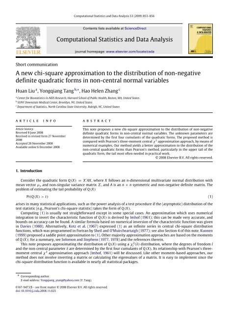
This note proposes a new chi-square approximation to the distribution of non-negative
definite quadratic forms in non-central normal variables. The unknown parameters are
determined by the first four cumulants of the quadratic forms. The proposed method is
compared with Pearson’s three-moment central χ 2 approximation approach, by means of
numerical examples. Our method yields a better approximation to the distribution of the
non-central quadratic forms than Pearson’s method, particularly in the upper tail of the
quadratic form, the tail most often needed in practical work.
© 2008 Elsevier B.V. All rights reserved.
Consider the quadratic form Q (X) = X ′ AX, where X follows an n-dimensional multivariate normal distribution with
mean vector µx and non-singular variance matrix Σ, and A is an n × n symmetric and non-negative definite matrix. The
problem of estimating the tail probability of Q (X)
Pr(Q (X) > t) (1)
arises in many statistical applications, such as the power analysis of a test procedure if the (asymptotic) distribution of the
test statistic (e.g., Pearson’s chi-square statistic) takes the form of Q (X).
Computing (1) is usually not straightforward except in some special cases. An approximation which uses numerical
integration to invert the characteristic function of Q (X) is derived by Imhof (1961); this can be made very accurate, and
bounds on accuracy can be found. A similar formula based on numerical inversion of the characteristic function was given
in Davies (1980). Alternatively, Kotz et al. (1967) expressed (1) as an infinite series in central chi-square distribution
functions, which was programmed in Fortran by Sheil and O’Muircheartaigh (1977); see also Section 4 of this note. Kuonen
(1999) proposed a saddle point approximation to (1). Other majority approximation approaches are based on the moments
of Q (X); for a summary, see Solomon and Stephens (1977, 1978) and the references therein.
This note proposes approximating the distribution of Q (X) using a χ 2
l (δ) distribution, where the degrees of freedom l
and the non-central parameter δ are determined by the first four cumulants of Q (X). Its relationship with Pearson’s threemoment
central χ 2 approximation approach (Imhof, 1961) will be discussed. Like other moment-based approaches, our
method does not involve inverting a matrix or calculating the eigenvalues of a matrix. It is easy to implement since the
chi-square distribution function is available in nearly all statistical packages.
∗ Corresponding author.
E-mail address: Yongqiang_ytang@yahoo.com (Y. Tang).
0167-9473/$ – see front matter © 2008 Elsevier B.V. All rights reserved.
doi:10.1016/j.csda.2008.11.025

854 H. Liu et al. / Computational Statistics and Data Analysis 53 (2009) 853–856
2. A new non-central chi-square approximation for Q (X)
2.1. Cumulants of the quadratic form
Let P be a n × n orthonormal matrix which converts B = Σ 1/2 AΣ 1/2 to the diagonal form Λ = diag(λ1, . . . , λn) = PBP ′ ,
where λ1 ≥ · · · ≥ λn ≥ 0. Let m = rank(A). If m < n, then λm+1 = · · · = λn = 0. Since Y = PΣ −1/2 X is normally
distributed with mean µy = PΣ −1/2 µx and variance In, Q (X) can be expressed as a weighted sum of chi-square variables:
Q (X) = X ′ AX = Y ′ ΛY =
n�
i=1
λiχ 2
h i (δi) =
m�
i=1
λiχ 2
h i (δi), (2)
where hi = 1, δi = µ 2
yi , and µyi is the ith component of µy for i = 1, . . . , m. The cumulant generating function of Q (X) is
given by (Imhof, 1961)
K(t) = 1
m�
m� δiλit
hi log(1 − 2tλi) +
2
1 − 2λit .
i=1
i=1
The formula for the kth cumulant of Q (X) is
κk = 2 k−1 �
m�
(k − 1)! λ k
i hi
m�
+ k
i=1
i=1
λ k
i δi
It is unnecessary to calculate the λi’s and δi’s explicitly since
m�
λ k
i hi = trace(Λ k ) = trace((PBP ′ ) k ) = trace(B k ) = trace((AΣ) k )
and
i=1
m�
i=1
λ k
i δi = µ ′ y Λk µy = µ ′ x Σ−1/2 P ′ (PBP ′ ) k PΣ −1/2 µx = µ ′ x (AΣ)k−1 Aµx.
The mean, standard deviation, skewness and kurtosis of Q (X) are given by
µQ = κ1 = c1, σQ = √ κ2 = � 2c2, β1 = κ3
�
. (3)
κ 3/2
2
where ck = �m i=1 λk
i hi + k �m i=1 λk
i δi, s1 = c3/c 3/2
2 and s2 = c4/c 2
2 .
2.2. The new approach
= √ 8s1, β2 = κ4
κ 2 = 12s2,
2
We propose using a non-central χ 2
l (δ) distribution to approximate the distribution of
Q (X) =
m�
i=1
λiχ 2
h i (δi).
We shall not impose the restriction hi = 1. The tail probability (1) is approximated by
�
Q (X) − µQ
Pr(Q (X) > t) = Pr
> t ∗
�
≈ Pr
σQ
� 2 χl (δ) − µχ
where t ∗ = (t − µQ )/σQ , µχ = E(χ 2
l (δ)) = l + δ, σχ =
l are determined so that the skewnesses of Q (X) and χ 2
l
χ 2
l
σχ
> t ∗
�
= Pr � χ 2
l (δ) > t∗ �
σχ + µχ
�
var(χ 2
l (δ)) = √ 2 a, and a = √ l + 2δ. The parameters δ and
(δ) are equal and the difference between the kurtoses of Q (X) and
(δ) is minimized. The solution to (4) will be given in (5) and (6) below.
The skewness of χ 2
l (δ) is √ 8(a 2 + δ)/a 3 , and that of Q (X) is √ 8s1. Since the two skewnesses are equal, we obtain
δ = s1a 3 − a 2 . Note that δ ≥ 0. Thus a ≥ 1/s1. The difference in kurtosis of Q (X) and χ 2
l (δ) is
�
� �
� 12(l
∆K = �
+ 4δ) � ��
�2 � − 12s2
� � 1
(l + 2δ) 2 � = 12 � − s1 + s2 − s
� a 2
�
�
�
1�
� .
(4)

If s 2
H. Liu et al. / Computational Statistics and Data Analysis 53 (2009) 853–856 855
1 > s2, the minimum value of ∆K is 0 when s 2
1 − s2 = (1/a − s1) 2 . Thus
� �
a = 1/ s1 − s 2
�
1 − s2 , δ = s1a 3 − a 2
If s 2
1 ≤ s2, ∆K is minimized when a = 1/s1. The final solution is given by
δ = s1a 3 − a 2 = 0 and l = a 2 − 2δ = 1/s 2
1 = c3
2 /c2
3
We can show that l > 0 and δ > 0 in (5) and that l > 0 and δ = 0 in (6).
2.3. Relation to Pearson’s central χ 2 approximation
and l = a 2 − 2δ. (5)
. (6)
Our method is closely related to Pearson’s three-moment central χ 2 approximation approach. The Pearson (1959)
approach was originally developed for approximating a non-central χ 2
l
Pr
where χ 2
l
Q (X):
� 2 χl (δ) − µχ
σχ
> t ∗
� � 2 χl ≈ Pr √
2l∗ ∗ − l∗
> t∗
2
(δ) distribution by a central χl∗ distribution:
�
, (7)
2 (δ) and χ ∗ have equal skewnesses. Imhof (1961) extended Pearson’s method to the non-negative quadratic form
Pr(Q (X) > t) = Pr
where l ∗ = 1/s 2
1
l
� Q (X) − µQ
σQ
� 2 χl ≈ Pr √
2l∗ ∗ − l∗
> t∗
> t ∗
�
�
�
= Pr χ 2
l∗ > l∗ + t ∗√ 2l∗ �
, (8)
2
is determined so that Q (X) and χl∗ have equal skewnesses. Although it is difficult to assess in a mathematical
way, the accuracy of Pearson’s approximation has been demonstrated in many empirical studies (Johnson, 1959; Imhof,
1961; Solomon and Stephens, 1977; Kuonen, 1999).
The accuracy of our approach is guaranteed since the approximation error of (4) is bounded by the sum of the
approximation errors of (7) and (8):
�
�
�
�Pr �
Q (X) − µQ
> t
σQ
∗
� � 2 χl (δ) − µχ
− Pr
> t
σχ
∗
��
���
�
�
≤ �
�Pr �
Q (X) − µQ
> t
σQ
∗
� � �� �
2 χl∗ − l∗ ��� �
− Pr √ > t∗ + �
2l∗ �Pr � � � 2
2
χl∗ − l∗
χl (δ) − µχ
√ > t∗ − Pr
> t
2l∗ σχ
∗
��
���
.
Note that this bound is quite conservative. In the next section, we will use a simulation study to show that the actual
approximation error of our method is usually much smaller than that of Pearson’s method.
Pearson’s method essentially uses the central χ 2 approximation by requiring the match of the third-order moments.
The proposed method considers a broader class of non-central χ 2 (δ) distributions, and searches for the distribution which
not only matches the third-order moments but also has the best match of the fourth-order moments. The better high-order
moment approximation often improves the tail probability approximation in practice. Our method is equivalent to Pearson’s
approach when s 2
1 ≤ s2. For central quadratic forms (δi = 0 for i = 1, . . . , m), the Cauchy–Schwarz inequality implies that
s 2
1 ≤ s2. Our method produces the exact tail probability when λ1 = · · · = λm; under this assumption, Q (X)/λ1 follows a
non-central chi-square distribution.
3. Numerical examples
This section numerically compares our method with Pearson’s three-moment χ 2 approximation method. The tail
probabilities of chi-square distributions are evaluated using the CDF function in SAS. Since Q (X) has the same distribution as
Q (z) = �m �hi i=1 j=1 λi
�
zij + √ �2, δi/hi where the zij’s are independent standard normal variables, an application of Eq. (144)
of Kotz et al. (1967) yields an exact formula for computing (1):
∞�
�
Pr(Q (X) > t) = ck Pr χ 2
�
t
> , (9)
2k+˜h β
k=0
for any 0 < β ≤ min(λ1, . . . , λm), where ˜h = � m
i=1 hi, γi = 1 − β/λi, gk = �� m
i=1
hiγ k
i + k � m
i=1
k−1
δiγi (1 − γi) � /2,
d = � m
i=1 (β/λi) h i/2 , e = � m
i=1 δi, c0 = d exp(−e/2), and ck = k −1 � k−1
r=0 gk−rcr for k ≥ 1. If the series is truncated after N
terms, the truncation error is bounded by
∞�
�
ck Pr χ 2
�
t
> ≤
2k+˜h β
∞�
ck = 1 −
k=N+1
k=N+1
N�
ck.
k=1

856 H. Liu et al. / Computational Statistics and Data Analysis 53 (2009) 853–856
Table 1
Probability that the quadratic form exceeds t. P1: exact values with accuracy 0.000001; P2: the proposed non-central χ 2 approximation; E2: the absolute
error for the proposed method; P3: Pearson’s central χ 2 approximation; E3: the absolute error for Pearson’s approximation.
Quadratic form t P1 P2 E2 P3 E3 E3/E2
2 (1) + .4χ2 (.6)
+ .1χ
2 .457461 .457753 .000292 .458967 .001507 5.2
2
1 (.8) 6
8
.031109
.006885
.031079
.006883
.000030
.000002
.030929
.006908
.000180
.000023
6.0
8.1
2 (6) + .3χ1 (2) 1
6
.954873
.407565
.955046
.407587
.000173
.000022
.951516
.408359
.003357
.000794
19.0
36.2
15 .022343 .022340 .000003 .022294 .000049 14.2
(1) 2 .347939 .347946 .000007 .357398 .009459 1342.3
+ .005χ 2
2 (1) 8
12
.033475
.006748
.033475
.006748
.000000
.000000
.032348
.006807
.001132
.000059
3677.2
2132.3
2 (6) + .15χ1 (2)
+ .35χ
3.5 .956318 .956315 .000003 .955961 .000357 100.3
2
2
6 (6) + .15χ2 (2) 8
13
.415239
.046231
.415248
.046228
.000009
.000002
.415273
.046085
.000034
.000146
4.0
59.8
Q1 = .5χ 2
1
Q2 = .7χ 2
1
Q3 = .995χ 2
1
Q4 = .35χ 2
1
In Table 1, all quadratic forms satisfy s 2
1 > s2. The exact tail probability is calculated using (9). As expected, our method
yields better approximation to the distribution of Q (X) than Pearson’s method, especially in the upper tail of Q (X). In all
examples given in Table 1, the absolute errors for Pearson’s approximation are at least three times as large as those for the
proposed method.
References
Davies, R.B., 1980. Algorithm as 155: The distribution of a linear combination of χ 2 random variables. Applied Statistics 29, 323–333.
Imhof, J.P., 1961. Computing the distribution of quadratic forms in normal variables. Biometrika 48, 419–426.
Johnson, N.L., 1959. On an extension of the connection between Poisson and χ 2 distributions. Biometrika 46, 352–363.
Kotz, S., Johnson, N.L., Boyd, D.W., 1967. Series representations of distributions of quadratic forms in normal variables ii. non-central case. The Annals of
Mathematical Statistics 38, 838–848.
Kuonen, D., 1999. Saddlepoint approximations for distributions of quadratic forms in normal variables. Biometrika 86, 929–935.
Pearson, E.S., 1959. Note on an approximation to the distribution of non-central χ 2 . Biometrika 46, 364.
Sheil, J., O’Muircheartaigh, I., 1977. Algorithm as 106: The distribution of non-negative quadratic forms in normal variables. Applied Statistics 26, 92–98.
Solomon, H., Stephens, M.A., 1977. Distribution of a sum of weighted chi-square variables. Journal of the American Statistical Association 72, 881–885.
Solomon, H., Stephens, M.A., 1978. Approximations to density functions using Pearson curves. Journal of the American Statistical Association 73, 153–160.