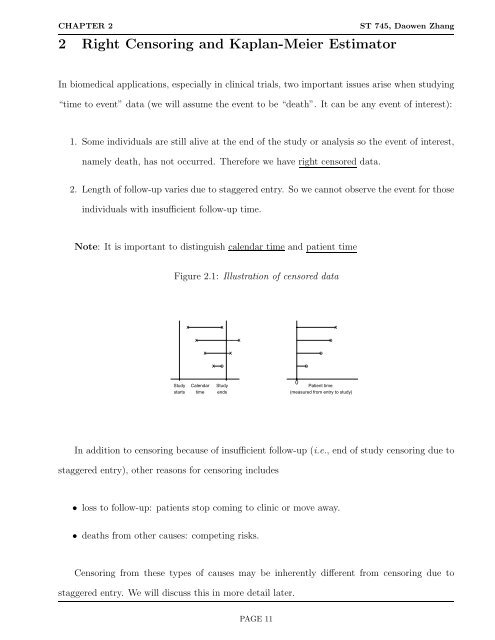
2 Right Censoring and Kaplan-Meier Estimator - NCSU Statistics

CHAPTER 2 ST 745, Daowen Zhang 

2 Right Censoring and Kaplan-Meier Estimator 

In biomedical applications, especially in clinical trials, two important issues arise when studying 

“time to event” data (we will assume the event to be “death”. It can be any event of interest): 

1. Some individuals are still alive at the end of the study or analysis so the event of interest, 

namely death, has not occurred. Therefore we have right censored data. 

2. Length of follow-up varies due to staggered entry. So we cannot observe the event for those 

individuals with insufficient follow-up time. 

Note: It is important to distinguish calendar time and patient time 

Figure 2.1: Illustration of censored data 

x x 

x x 

x x 

x o 

Study Calendar Study 

starts time ends 

0 

Patient time 

(measured from entry to study) 

In addition to censoring because of insufficient follow-up (i.e., end of study censoring due to 

staggered entry), other reasons for censoring includes 

• loss to follow-up: patients stop coming to clinic or move away. 

• deaths from other causes: competing risks. 

Censoring from these types of causes may be inherently different from censoring due to 

staggered entry. We will discuss this in more detail later. 

PAGE 11 

o 

o 

o 

x


Censoring and differential follow-up create certain difficulties in the analysis for such data 

as is illustrated by the following example taken from a clinical trial of 146 patients treated after 

they had a myocardial infarction (MI). 

The data have been grouped into one year intervals and all time is measured in terms of 

patient time. 

Table 2.1: Data from a clinical trial on myocardial infarction (MI) 

Number alive and under 

Year since observation at beginning Number dying Number censored 

entry into study of interval during interval or withdrawn 

[0, 1) 146 27 3 

[1, 2) 116 18 10 

[2, 3) 88 21 10 

[3, 4) 57 9 3 

[4, 5) 45 1 3 

[5, 6) 41 2 11 

[6, 7) 28 3 5 

[7, 8) 20 1 8 

[8, 9) 11 2 1 

[9, 10) 8 2 6 

Question: Estimate the 5 year survival rate, i.e., S(5) = P [T ≥ 5]. 

Two naive and incorrect answers are given by 

1. � F (5) = P [T


1. The first estimate would be correct if all censoring occurred after 5 years. Of cause, this 

was not the case leading to overly optimistic estimate (i.e., overestimatesS(5)). 

2. The second estimate would be correct if all individuals censored in the 5 years were censored 

immediately upon entering the study. This was not the case either, leading to overly 

pessimistic estimate (i.e., underestimates S(5)). 

Our clinical colleagues have suggested eliminating all individuals who are censored and use 

the remaining “complete” data. This would lead to the following estimate 

�F (5) = P [T ≤ 5] = 

76 deaths in 5 years 

146 -60 (censored) =88.4%, 

This is even more pessimistic than the estimate given by (2). 

Life-table Estimate 

� S(5) = 1 − � F (5) = 11.6%. 

More appropriate methods use life-table or actuarial method. The problem with the above 

two estimates is that they both ignore the fact that each one-year interval experienced censoring 

(or withdrawing). Obviously we need to take this information into account in order to reduce 

bias. If we can express S(5) as a function of quantities related to each interval and get a very 

good estimate for each quantity, then intuitively, we will get a very good estimate of S(5). By 

the definition of S(5), we have: 

S(5) = P [T ≥ 5] = P [(T ≥ 5) ∩ (T ≥ 4)] = P [T ≥ 4] · P [T ≥ 5|T ≥ 4] 

= P [T ≥ 4] ·{1 − P [4 ≤ T


Table 2.2: Life-table estimate of S(5) assuming censoring occurred at the end of interval 

duration [ti−1,ti) n(x) d(x) w(x) �m(x) = d(x) 

n(x) 1 − �m(x) � S R (ti) = � (1 − �m(x)) 

[0, 1) 146 27 3 0.185 0.815 0.815 

[1, 2) 116 18 10 0.155 0.845 0.689 

[2, 3) 88 21 10 0.239 0.761 0.524 

[3, 4) 57 9 3 0.158 0.842 0.441 

[4, 5) 45 1 3 0.022 0.972 0.432 

Case 1: Let us first assume that anyone censored in an interval of time is censored at the 

end of that interval. Then we can estimate each qi =1− m(i − 1) in the following way: 

d(0) ∼ Bin(n(0),m(0)) =⇒ �m(0) = d(0) 

n(0) 

d(1)|H ∼ Bin(n(1),m(1)) =⇒ �m(1) = d(1) 

n(1) 

··· 

= 27 

146 =0.185, �q1 =1− �m(0) = 0.815 

where H means data history (i.e, data before the second interval). 

= 18 

116 =0.155, �q2 =1− �m(1) = 0.845 

The life table estimate would be computed as shown in Table 2.2. So the 5 year survival 

probability estimate � S R (5) = 0.432. (If the assumption that anyone censored in an in- 

terval of time is censored at the end of that interval is true, then the estimator � S R (5) is 

approximately unbiased to S(5).) 

Of course, this estimate � S R (5) will have variation since it was calculated from a sample. We 

need to estimate its variation in order to make inference on S(5) (for example, construct a 

95% CI for S(5)). 

However, � S R (5) is a product of 5 estimates (�q1 – �q5), whose variance is not easy to find. 

But we have 

log( � S R (5)) = log(�q1)+log(�q2)+log(�q3)+log(�q4)+log(�q5). 

So if we can find out the variance of each log(�qi), we might be able to find out the variance 

PAGE 14


of log( � S R (5)) and hence the variance of � S R (5). 

For this purpose, let us first introduce a very popular method in statistics: delta method: 

If 

Delta Method: 

� θ a ∼ N(θ, σ 2 ) 

then f( � θ) a ∼ N(f(θ), [f ′ (θ)] 2 σ 2 ) 

Proof of delta method: If σ 2 is small, � θ will be close to θ with high probability. We hence 

can expand f( � θ)aboutθ using Taylor expansion: 

f( � θ) ≈ f(θ)+f ′ (θ)( � θ − θ). 

We immediately get the (asymptotic) distribution of f( � θ) from this expansion. 

Returning to our problem. Let � φi = log(�qi). Using the delta method, the variance of � φi 

is approximately equal to 

var( � � 

1 

φi) = 

qi 

� 2 

var( �qi). 

Therefore we need to find out and estimate var(�qi). Of course, we also need to find out the 

covariances among � φi and � φj (i �= j). For this purpose, we need the following theorem: 

Double expectation theorem (Law of iterated conditional expectation and variance): If X and 

Y are any two random variables (or vectors), then 

Since �qi =1− �m(i − 1), we have 

E(X) = E[E(X|Y )] 

Var(X) =Var[E(X|Y )] + E[Var(X|Y )] 

var( �qi) = var(�m(i − 1)) 

PAGE 15


which can be estimated by 

= E[var(�m(i−1)|H)] + var[E(�m(i − 1)|H)] 

� � 

m(i − 1)[1 − m(i − 1)] 

= E 

+var[m(i−1)] n(i − 1) 

� � 

1 

= m(i − 1)[1 − m(i − 1)]E , 

n(i − 1) 

�m(i − 1)[1 − �m(i − 1)] 

. 

n(i − 1) 

Hence the variance of � φi = log(�qi) can be approximately estimated by 

� �2 1 �m(i − 1)[1 − �m(i − 1)] 

= 

n(i − 1) 

�qi 

�m(i − 1) 

[1 − �m(i − 1)]n(i − 1) = 

d 

(n − d)n . 

Now let us look at the covariances among � φi and � φj (i �= i). It is very amazing that they 

are all approximately equal to zero! 

For example, let us consider the covariance between � φ1 and � φ2. Since � φ1 = log(�q1) and 

�φ2 = log(�q2), using the same argument for the delta method, we know that we only need 

to find out the covariance between �q1 and �q2, or equivalently, the covariance between �m(0) 

and �m(1). This can be seen from the following: 

E[�m(0)�m(1)] = E[E[�m(0)�m(1)|n(0),d(0),w(0)]] 

= E[�m(0)E[�m(1)|n(0),d(0),w(0)]] 

= E[�m(0)m(1)] 

= m(1)E[�m(0)] 

= m(1)m(0) = E[�m(0)]E[�m(1)]. 

Therefore, the covariance between �m(0) and �m(1) is zero. Similarly, we can show other 

covariances are zero. Hence, 

var(log( � S R (5))) = var( � φ1)+var( � φ2)+var( � φ3)+var( � φ4)+var( � φ5). 

Let � θ = log( � S R (5)). Then � S R (5) = e �θ .So 

var( � S R (5)) = (e θ ) 2 var(log( � S R (5))) = (S(5)) 2 [var( � φ1)+var( � φ2)+var( � φ3)+var( � φ4)+var( � φ5)], 

PAGE 16


which can be estimated by 

�var( � S R (5)) = ( � S R (5)) 2 

� 

d(0) 

(n(0) − d(0))n(0) + 

i=0 

d(1) 

(n(1) − d(1))n(1) + 

d(2) 

(n(2) − d(2))n(2) 

d(3) 

+ 

(n(3) − d(3))n(3) + 

= 

� 

d(4) 

(n(4) − d(4))n(4) 

( � S R (5)) 2 

4� d(i) 

. 

[n(i) − d(i)]n(i) 

(2.1) 

Case 2: Let us assume that anyone censored in an interval of time is censored right at the 

beginning of that interval. Then the life table estimate would be computed as shown in 

Table 2.3. So the 5 year survival probability estimate = 0.400. (In this case, the estimator 

�S L (5) is approximately unbiased to S(5).) 

The variance estimate of � S L (5) is similar to that of � S R (5)exceptthatweneedtochange 

the “sample size” for each mortality estimate to n − w in equation (2.1). 

Table 2.3: Life-table estimate of S(5) assuming censoring occurred at the beginning of interval 

duration [ti−1,ti) n(x) d(x) w(x) �m(x) = d(x) 

n(x)−w(x) 1 − �m(x) � S L (ti) = � (1 − �m(x)) 

[0, 1) 146 27 3 0.189 0.811 0.811 

[1, 2) 116 18 10 0.170 0.830 0.673 

[2, 3) 88 21 10 0.269 0.731 0.492 

[3, 4) 57 9 3 0.167 0.833 0.410 

[4, 5) 45 1 3 0.024 0.976 0.400 

The naive estimates range from 35% to 47.9% for the five year survival probability with the 

“complete case” (i.e., eliminating anyone censored) estimator giving an estimate of 11.6%. 

The life-table estimate ranged from 40% to 43.2% depending on whether we assume censoring 

occurred at the left (i.e., beginning) or right (i.e., end) of each interval. 

More than likely censoring occurs during the interval. Thus � S L and � S R are not correct. A 

compromise is to use the following modification: 

PAGE 17


Table 2.4: Life-table estimate of S(5) assuming censoring occurred during the interval 

duration [ti−1,ti) n(x) d(x) w(x) �m(x) = 

d(x) 

n(x)−w(x)/2 1 − �m(x) � S LT (ti) = � (1 − �m(x)) 

[0, 1) 146 27 3 0.187 0.813 0.813 

[1, 2) 116 18 10 0.162 0.838 0.681 

[2, 3) 88 21 10 0.253 0.747 0.509 

[3, 4) 57 9 3 0.162 0.838 0.426 

[4, 5) 45 1 3 0.023 0.977 0.417 

That is, when calculating the mortality estimate in each interval, we use (n(x) − w(x)/2) as 

the “sample size”. This number is often referred to as the effective sample size. 

So the 5 year survival probability estimate � S LT (5) = 0.417, which is between � S L =0.400 and 

�S R =0.432. 

Figure 2.2: Life-table estimate of the survival probability for MI data 

Survival probability 

0.2 0.4 0.6 0.8 1.0 

0 2 4 6 8 10 

Time (years) 

Figure 2.2 shows the life-table estimate of the survival probability assuming censoring oc- 

curred during interval. Here the estimates were connected using straight lines. No special 

significance should be given to this. From this figure, the median survival time is estimated to 

PAGE 18


be about 3 years. 

The variance estimate of the life-tabble estimate � S LT (5) is similar to equation (2.1) except 

that the sample size n(i) is changed to n(i) − w(i)/2. That is 

�var( � S LT (5)) = ( � S LT (5)) 2 

4� 

i=0 

d(i) 

. (2.2) 

[n(i) − w(i)/2 − d(i)][n(i) − w(i)/2] 

Of course, we can also use the above formula to calculate the variance of � S LT (t) atother 

time points. For example: 

�var( � S LT (1)) = ( � S LT (1)) 2 

� 

� 

d(0) 

[n(0) − w(0)/2 − d(0)][n(0) − w(0)/2] 

= 0.813 2 27 

× 

(146 − 3/2 − 27)(146 − 3/2) =0.8132 × 0.001590223 = 0.001051088. 

Therefore SE( � S LT (1)) = √ 0.001051088 = 0.0324. 

The calculation presented in Table 2.4 can be implemented using Proc Lifetest in SAS: 

options ls=72 ps=60; 

Data mi; 

input survtime number status; 

cards; 

0 27 1 

0 3 0 

1 18 1 

1 10 0 

2 21 1 

2 10 0 

3 9 1 

3 3 0 

4 1 1 

4 3 0 

5 2 1 

5 11 0 

6 3 1 

6 5 0 

7 1 1 

7 8 0 

8 2 1 

8 1 0 

9 2 1 

9 6 0 

; 

proc lifetest method=life intervals=(0 to 10 by 1); 

time survtime*status(0); 

freq number; 

run; 

PAGE 19


Note that the number of observed events and withdrawals in [ti−1,ti) were entered after ti−1 

instead of ti. Part of the output of the above SAS program is 

The LIFETEST Procedure 

Life Table Survival Estimates 

Effective Conditional 

Interval Number Number Sample Probability 

[Lower, Upper) Failed Censored Size of Failure 

0 1 27 3 144.5 0.1869 

1 2 18 10 111.0 0.1622 

2 3 21 10 83.0 0.2530 

3 4 9 3 55.5 0.1622 

4 5 1 3 43.5 0.0230 

5 6 2 11 35.5 0.0563 

6 7 3 5 25.5 0.1176 

7 8 1 8 16.0 0.0625 

8 9 2 1 10.5 0.1905 

9 10 2 6 5.0 0.4000 

Conditional 

Probability Survival Median 

Interval Standard Standard Residual 

[Lower, Upper) Error Survival Failure Error Lifetime 

0 1 0.0324 1.0000 0 0 3.1080 

1 2 0.0350 0.8131 0.1869 0.0324 4.4265 

2 3 0.0477 0.6813 0.3187 0.0393 5.2870 

3 4 0.0495 0.5089 0.4911 0.0438 . 

4 5 0.0227 0.4264 0.5736 0.0445 . 

5 6 0.0387 0.4166 0.5834 0.0446 . 

6 7 0.0638 0.3931 0.6069 0.0450 . 

7 8 0.0605 0.3469 0.6531 0.0470 . 

8 9 0.1212 0.3252 0.6748 0.0488 . 

9 10 0.2191 0.2632 0.7368 0.0558 . 

Here the numbers in the column under Conditional Probability of Failure are the es- 

timated mortality �m(x) =d(x)/(n(x) − w(x)/2). 

The above lifetable estimation can also be implemented using R. HereistheR code: 

> tis ninit nlost nevent lifetab(tis, ninit, nlost, nevent) 

PAGE 20


The output from the above R function is 

nsubs nlost nrisk nevent surv pdf hazard se.surv 

0-1 146 3 144.5 27 1.0000000 0.186851211 0.20610687 0.00000000 

1-2 116 10 111.0 18 0.8131488 0.131861966 0.17647059 0.03242642 

2-3 88 10 83.0 21 0.6812868 0.172373775 0.28965517 0.03933747 

3-4 57 3 55.5 9 0.5089130 0.082526440 0.17647059 0.04382194 

4-5 45 3 43.5 1 0.4263866 0.009801991 0.02325581 0.04452036 

5-6 41 11 35.5 2 0.4165846 0.023469556 0.05797101 0.04456288 

6-7 28 5 25.5 3 0.3931151 0.046248831 0.12500000 0.04503654 

7-8 20 8 16.0 1 0.3468662 0.021679139 0.06451613 0.04699173 

8-9 11 1 10.5 2 0.3251871 0.061940398 0.21052632 0.04879991 

9-10 8 6 5.0 2 0.2632467 NA NA 0.05579906 

se.pdf se.hazard 

0-1 0.032426423 0.03945410 

1-2 0.028930638 0.04143228 

2-3 0.033999501 0.06254153 

3-4 0.026163333 0.05859410 

4-5 0.009742575 0.02325424 

5-6 0.016315545 0.04097447 

6-7 0.025635472 0.07202769 

7-8 0.021195209 0.06448255 

8-9 0.040488466 0.14803755 

9-10 NA NA 

Note: Here the numbers in the column of hazard are the estimated hazard rates at the 

midpoint of each interval by assuming the true survival function S(t) is a straight line in each 

interval. You can find an explicit expression for this estimator using the relation 

λ(t) = f(t) 

S(t) , 

and the assumption that the true survival function S(t) is a straight line in [ti−1,ti): 

S(t) =S(ti−1)+ S(ti) − S(ti−1) 

ti − ti−1 

(t − ti−1), for t ∈ [ti−1,ti). 

These estimates are very close to the mortality estimates we obtained before (the column under 

Conditional Probability of Failure in the SAS output.) 

Kaplan-Meier Estimator 

The Kaplan-Meier or product limit estimator is the limit of the life-table estimator when 

intervals are taken so small that only at most one distinct observation occurs within an interval. 

Kaplan and Meier demonstrated in a paper in JASA (1958) that this estimator is “maximum 

likelihood estimate”. 

PAGE 21


Figure 2.3: An illustrative example of Kaplan-Meier estimator 

1.0 

0.8 

0.6 

0.4 

0.2 

0.0 

x 

4.5 

x 

7.5 

o x 

11.5 

13.5 

Patient time (years) 

o x 

x o x 

15.516.5 

1 − �m(x) 9 

8 

6 

4 

: 1 1 1 1 1 1 1 1 1 1 1 1 10 9 7 5 

�S(t) 9 

8 

48 

192 

: 1 1 1 1 . . . . . . . . 10 10 70 350 

19.5 

o 

3 

4 1 1 1 

2 1 1 

144 

350 . . 144 

700 . . 

We will illustrate through a simple example shown in Figure 2.3 how the Kaplan-Meier 

estimator is constructed. 

By convention, the Kaplan-Meier estimate is a right continuous step function which takes 

jumps only at the death time. 

The calculation of the above KM estimate can be implemented using Proc Lifetest in SAS 

as follows: 

Data example; 

input survtime censcode; 

cards; 

4.5 1 

7.5 1 

8.5 0 

11.5 1 

13.5 0 

15.5 1 

16.5 1 

17.5 0 

19.5 1 

21.5 0 

; 

Proc lifetest; 

PAGE 22


time survtime*censcode(0); 

run; 

And part of the output from the above program is 

The LIFETEST Procedure 

Product-Limit Survival Estimates 

Survival 

Standard Number Number 

SURVTIME Survival Failure Error Failed Left 

0.0000 1.0000 0 0 0 10 

4.5000 0.9000 0.1000 0.0949 1 9 

7.5000 0.8000 0.2000 0.1265 2 8 

8.5000* . . . 2 7 

11.5000 0.6857 0.3143 0.1515 3 6 

13.5000* . . . 3 5 

15.5000 0.5486 0.4514 0.1724 4 4 

16.5000 0.4114 0.5886 0.1756 5 3 

17.5000* . . . 5 2 

19.5000 0.2057 0.7943 0.1699 6 1 

21.5000* . . . 6 0 

* Censored Observation 

The above Kaplan-Meier estimate can also be obtained using R function survfit(). The 

code is given in the following: 

> survtime status fit summary(fit) 

Call: survfit(formula = Surv(survtime, status), conf.type = c("plain")) 

time n.risk n.event survival std.err lower 95% CI upper 95% CI 

4.5 10 1 0.900 0.0949 0.7141 1.000 

7.5 9 1 0.800 0.1265 0.5521 1.000 

11.5 7 1 0.686 0.1515 0.3888 0.983 

15.5 5 1 0.549 0.1724 0.2106 0.887 

16.5 4 1 0.411 0.1756 0.0673 0.756 

19.5 2 1 0.206 0.1699 0.0000 0.539 

Let d(x) denote the number of deaths at time x. Generally d(x) is either zero or one, but we 

allow the possibility of tied survival times in which case d(x) maybegreaterthanone.Letn(x) 

PAGE 23


denote the number of individuals at risk just prior to time x; i.e., number of individuals in the 

sample who neither died nor were censored prior to time x. Then Kaplan-Meier estimate can be 

expressed as 

KM(t) = � 

� 

1 − d(x) 

� 

. 

n(x) 

x≤t 

Note: In the notation above, the product changes only at times x where d(x) ≥ 1; , i.e., 

only at times where we observed deaths. 

Non-informative Censoring 

In order that the life-table estimates give unbiased results there is an important assumption 

that individuals who are censored are at the same risk of subsequent failure as those who are still 

alive and uncensored. The risk set at any time point (the individuals still alive and uncensored) 

should be representative of the entire population alive at the same time. If this is the case, the 

censoring process is called non-informative. Statistically, if the censoring process is indepen- 

dent of the survival time, then we will automatically have non-informative censoring. Actually, 

we almost always mean independent censoring by non-informative censoring. 

If censoring only occurs because of staggered entry, then the assumption of non-informative 

censoring seems plausible. However, when censoring results from loss to follow-up or death from 

a competing risk, then this assumption is more suspect. If at all possible censoring from these 

later situations should be kept to a minimum. 

Greenwood’s Formula for the Variance of the Life-table Estimator 

The derivation given below is heuristic in nature but will try to capture some of the salient 

feature of the more rigorous treatments given in the theoretical literature on survival analysis. 

For this reason, we will use some of the notation that is associated with the “counting process” 

approach to survival analysis. In fact we have seen it when we discussed the life-table estimator. 

PAGE 24


It is useful when considering the product limit estimator to partition time into many small 

intervals, say, with interval length equal to ∆x where ∆x is small. 

Figure 2.4: Partition of time axis 

Patient time 

Let “x” denote some arbitrary time point on the grid above and define 

• Y (x) = number of individuals at risk (i.e., alive and uncensored) at time point x. 

• dN(x) = number of observed deaths occurring in [x, x +∆x). 

Recall: Previously, Y (x) was denoted by n(x) anddN(x) was denoted by d(x). 

It should be straightforward to see that “w(x)”, the number of censored individuals in [x, x+ 

∆x), is equal to {[Y (x) − Y (x +∆x)] − dN(x)}. 

Note: In theory, we should be able to choose ∆x small enough so that {dN(x) > 0and 

w(x) > 0} should never occur. In practice, however, data may not be collected in that fashion, 

in which case, approximations such as those given with life-table estimators may be necessary. 

With these definitions, the Kaplan-Meier estimator can be written as 

� 

� 

KM(t) = 

1 − 

all grid points x such that x +∆x ≤ t 

dN(x) 

� 

, as ∆x → 0, 

Y (x) 

which can be modified if “∆x” is not chosen small enough to be 

� 

� 

� 

dN(x) 

LT (t) = 

1 − 

, 

Y (x) − w(x)/2 


where LT (t) means life-table estimator. 

If the sample size is large and ∆x is small, then dN(x) 

Y (x) is a small number (i.e., close to zero) 

and as long as x is not close to the right hand tail of the survival distribution (where Y (x) may 

PAGE 25 

x


be very small). If this is the case, then 

exp 

� 

− dN(x) 

Y (x) 

� 

≈ 

� 

1 − dN(x) 

Y (x) 

Here we used the approximation e x ≈ 1+x when x is close to zero. This approximation is exact 

when dN(x) 

Y (x) =0. 

Therefore, the Kaplan-Meier estimator can be approximated by 

� 

� 

KM(t) ≈ 

exp − 


dN(x) 

� � 

=exp − 

Y (x) 

� 

x


By the definition of a hazard function, 

λ(x)∆x ≈ P [x ≤ T


(b) Var[dN(x)|H(x)] = Y (x)π(x)[1 − π(x)], 

� � 

dN(x) � 

� 

(c) E � 

Y (x) � H(x) 

� 

= π(x), 

�� 

Y (x) dN(x) Y (x) − dN(x) �� 

(d) E 

H(x) = π(x)[1 − π(x)]. 

Y (x) − 1 Y (x) Y (x) 

Consider the Nelson-Aalen estimator � Λ(t) = � dN(x) 

x


We will first demonstrate that the cross product terms have expectation equal to zero. Let 

us take one such term and let us say, without loss of generality, that x


If we wanted to estimate π(x)[1−π(x)] 

, then using (2.d) we might think that 

Y (x) 

dN(x) 

Y (x) 

� � 

Y (x)−dN(x) 

Y (x) 

Y (x) − 1 

may be reasonable. In fact, we would then use as an estimate for Var( � Λ(t)) the following 

estimator; summing the above estimator over all grid points x such that x +∆x ≤ t. 

�Var( � Λ(t)) = � 

⎡ 

⎣ 

x


which is also written as 

Remark: 

� t 

0 

dN(x) 

Y 2 (x) . 

• We proved that the Nelson-Aalen estimator � dN(x) 

x


�Λ(t) is asymptotically normal with mean Λ(t) and variance Var[ � Λ(t)], which can be estimated 

unbiasedly by 

and in the case of no ties, by 

�Var( � Λ(t)) = � 

⎡ 

⎣ 

x


meaning that this random interval will cover the true value S(t) with probability 1 − α. 

An example: We will use the hypothetical data shown in Figure 2.3 to illustrate the calcu- 

lation of � Λ(t), � Var � Λ(t), and confidence intervals for Λ(t) andS(t). For illustration, let us take 

t = 17. Note that there are no ties in this example. So 

�Λ(t) = � 

x


Consequently, using the delta method we get 

�S(t) a ∼ N(S(t), [S(t)] 2 Var[ � Λ(t)]), 

and a (1 − α)th confidence interval for S(t) isgivenby 

�S(t) ± zα/2{ � S(t) ∗ se[ � Λ(t)]}. 

Remark: Note that [S(t)] 2 Var[ � Λ(t)] is an estimate of Var[ � S(t)], where � S(t) =exp[− � Λ(t)]. 

Previously, we showed that the Kaplan-Meier estimator 

KM(t) = � 

� 

1 − dN(x) 

� 

Y (x) 

x


is 

e −�Λ(t) ± 1.96 ∗ e −�Λ(t) se[ � Λ(t)] = e −0.801 ± 1.96 ∗ e −0.801 ∗ 0.381 = [0.114, 0.784]. 

The estimated se[ � S(t)] = 0.171. 

If we use the Kaplan-Meier estimator, together with Greenwood’s formula for estimating the 

variance, to construct a 95% confidence interval for S(t), we would get 

� 

KM(t) = 1 − 1 

�� 

1 − 

10 

1 

�� 

1 − 

9 

1 

�� 

1 − 

7 

1 

�� 

1 − 

5 

1 

� 

=0.411 

4 

�Var[KM(t)] = 0.411 2 

� � 

1 1 1 1 1 

+ + + + =0.03077 

10 ∗ 9 9 ∗ 8 7 ∗ 6 5 ∗ 4 4 ∗ 3 

�se[KM(t)] = √ 0.03077 = 0.175 

�Var[ � ΛKM(t)] = 

1 1 1 1 1 

+ + + + 

10 ∗ 9 9 ∗ 8 7 ∗ 6 5 ∗ 4 4 ∗ 3 =0.182 

se[ � ΛKM(t)] = 0.427. 

Thus a 95% confidence interval for S(t) isgivenby 

KM(t) ± 1.96 ∗ �se[KM(t)] = 0.411 ± 1.96 ∗ 0.175 = [0.068, 0.754], 

which is close to the confidence interval using delta method, considering the sample size is only 10. 

In fact the estimated standard errors for � S(t) andKM(t) using delta method and Greenwood’s 

formula are 0.171 and 0.175 respectively, which agree with each other very well. 

Note: IfwewanttouseR function survfit() to construct a confidence interval for S(t)with 

the form KM(t) ± zα/2 ∗ �se[KM(t)],wehavetospecifytheargumentconf.type=c("plain") 

in survfit(). The default constructs the confidence interval for S(t) by exponentiating the 

confidence interval for the cumulative hazard using the Kaplan-Meier estimator. For example, 

a 95% CI for S(t) isKM(t) ∗ [e −1.96∗se[�ΛKM(t)] ,e 1.96∗se[�ΛKM(t)] ]=0.411 ∗ [e −1.96∗0.427 , [e 1.96∗0.427 ]= 

[0.178, 0.949]. 

Comparison of confidence intervals for S(t) 

1. exponentiating the 95% CI for cumulative hazard using Nelson-Aalen estimator: [0.212, 0.944]. 

PAGE 35


2. Delta-method using Nelson-Aalen estimator: [0.114, 0.784]. 

3. exponentiating the 95% CI for cumulative hazard using Kaplan-Meier estimator: [0.178, 0.949]. 

4. Kaplan-Meier estimator together with Greenwood’s formula for variance: [0.068, 0.754]. 

These are relatively close and the approximations become better with larger sample sizes. 

Of the different methods for constructing confidence intervals, “usually” the most accurate 

is based on exponentiating the confidence intervals for the cumulative hazard function based on 

Nelson-Aalen estimator. We don’t feel that symmetry is necessarily an important feature that 

confidence interval need have. 

Summary 

1. We first estimate S(t) byKM(t) = � � 

x


Estimators of quantiles (such as median, first and third quartiles) of a distribution can be 

obtained by inverse relationships. This is most easily illustrated through an example. 

Suppose we want to estimate the median S −1 (0.5) or any other quantile ϕ = S −1 (θ); 0 < 

θ


Similarly, we can show that 

Therefore, 

P [S( �ϕL)


6.5206 7 1 0.202 0.0663 0.1065 0.385 

7.1127 6 1 0.169 0.0632 0.0809 0.352 

9.3017 3 1 0.112 0.0623 0.0379 0.333 

11.1589 1 1 0.000 NA NA NA 

The true survival time has an exponential distribution with λ =0.2/year (so the true mean 

is 5 years and median is 5 ∗ log(2) ≈ 3.5 years). The (potential) censoring time is independent 

from the survival time and has an exponential distribution with λ =0.1/year (so it is stochas- 

tically larger than the survival time). The Kaplan estimate (solid line) and its 95% confidence 

intervals (dotted lines) are shown in Figure 2.5, which is generated using R function plot(fit, 

xlab="Patient time (years)", ylab="survival probability"). Note that these CIs are 

constructed by exponentiating the CIs for Λ(t). From this figure, the median survival time is 

estimated to be 3.56 years, with its 95% confidence interval [2.51, 6.20]. 

Figure 2.5: Illustration for constructing 95% CI for median survival time 

survival probability 

0.0 0.2 0.4 0.6 0.8 1.0 

2.51 3.56 

6.20 

0 2 4 6 8 10 


If we use symmetric confidence intervals of S(t) to construct the confidence interval for the 

median of the true survival time, then we need to specify conf.type=c("plain") in survfit() 

as follows 

> fit


> summary(fit) 

Call: survfit(formula = Surv(obstime, status), conf.type = c("plain")) 

time n.risk n.event survival std.err lower 95% CI upper 95% CI 

0.0747 50 1 0.980 0.0198 0.9412 1.000 

0.0908 49 1 0.960 0.0277 0.9057 1.000 

0.4332 46 1 0.939 0.0341 0.8723 1.000 

0.4420 45 1 0.918 0.0392 0.8414 0.995 

0.5454 44 1 0.897 0.0435 0.8121 0.983 

0.6126 43 1 0.877 0.0472 0.7839 0.969 

0.7238 42 1 0.856 0.0505 0.7567 0.955 

1.1662 40 1 0.834 0.0536 0.7292 0.939 

1.2901 39 1 0.813 0.0563 0.7025 0.923 

1.3516 38 1 0.791 0.0588 0.6763 0.907 

1.4490 37 1 0.770 0.0609 0.6506 0.890 

1.6287 35 1 0.748 0.0630 0.6245 0.872 

1.8344 34 1 0.726 0.0649 0.5988 0.853 

1.9828 33 1 0.704 0.0666 0.5736 0.835 

2.1467 32 1 0.682 0.0680 0.5487 0.815 

2.3481 31 1 0.660 0.0693 0.5242 0.796 

2.4668 30 1 0.638 0.0704 0.5001 0.776 

2.5135 29 1 0.616 0.0713 0.4763 0.756 

2.5999 28 1 0.594 0.0721 0.4528 0.735 

2.9147 27 1 0.572 0.0727 0.4296 0.715 

2.9351 25 1 0.549 0.0733 0.4055 0.693 

3.2168 24 1 0.526 0.0737 0.3818 0.671 

3.4501 22 1 0.502 0.0742 0.3570 0.648 

3.5620 21 1 0.478 0.0744 0.3326 0.624 

3.6795 20 1 0.455 0.0744 0.3087 0.600 

3.8475 18 1 0.429 0.0744 0.2834 0.575 

4.8888 16 1 0.402 0.0745 0.2565 0.548 

5.3910 15 1 0.376 0.0742 0.2302 0.521 

6.1186 14 1 0.349 0.0736 0.2046 0.493 

6.1812 13 1 0.322 0.0726 0.1796 0.464 

6.1957 12 1 0.295 0.0714 0.1552 0.435 

6.2686 10 1 0.266 0.0701 0.1283 0.403 

6.3252 9 1 0.236 0.0682 0.1024 0.370 

6.5206 7 1 0.202 0.0663 0.0724 0.332 

7.1127 6 1 0.169 0.0632 0.0447 0.293 

9.3017 3 1 0.112 0.0623 0.0000 0.235 

11.1589 1 1 0.000 NA NA NA 

The Kaplan estimate (solid line) and its symmetric 95% confidence intervals (dotted lines) are 

shown in Figure 2.6. Note that the Kaplan estimate is the same as before. From this figure, the 

median survival time is estimated to be 3.56 years, with its 95% confidence interval [2.51, 6.12]. 

Note: If we treat the censored data obstime as uncensored and fit an exponential model 

to it, then the “best” estimate of the median survival time is 2.5, with 95% confidence interval 

[1.8, 3.2] (using the methodology to be presented in next chapter). These estimates severely 

underestimate the true median survival time 3.5 years. 

PAGE 40


Figure 2.6: Illustration for constructing 95% CI for median survival time using symmetric CIs 

of S(t) 

Note: 

survival probability 

0.0 0.2 0.4 0.6 0.8 1.0 

2.51 3.56 

6.12 

0 2 4 6 8 10 


If we want a CI for the quantile such as the median survival time with a different confidence 

level, say, 90%, then we need to construct 90% confidence intervals for S(t). This can be done 

by specifying conf.int=0.9 in the R function survfit(). 

If we use Proc Lifetest in SAS to compute the Kaplan-Meier estimate, it will produce 95% 

confidence intervals for 25%, 50% (median) and 75% quantiles of the true survival time. 

Other types of censoring and truncation: 

• Left censoring: This kind of censoring occurs when the event of interest is only known to 

happen before a specific time point. For example, in a study of time to first marijuana use 

(example 1.17, page 17 of Klein & Moeschberger) 191 high school boys were asked “when 

did you first use marijuana?”. Some answers were “I have used it but cannot recall when 

the first time was”. For these boys, their time to first marijuana use is left censored at 

their current age. For the boys who never used marijuana, their time to first marijuana use 

is right censored at their current age. Of course, we got their exact time to first marijuana 

PAGE 41


use for those boys who remembered when they first used it. 

• Interval censoring occurs when the event of interest is only known to take place in an 

interval. For example, in a study to compare time to cosmetic deterioration of breasts 

for breast cancer patients treated with radiotherapy and radiotherapy + chemotherapy, 

patients were examined at each clinical visit for breast retraction and the breast retraction 

is only known to take place between two clinical visits or right censored at the end of the 

study. See example 1.18 on page 18 of Klein & Moeschberger. 

• Left truncation occurs when the time to event of interest in the study sample is greater 

than a (left) truncation variable. For example, in a study of life expectancy (survival time 

measured from birth to death) using elderly residents in a retirement community (example 

1.16, page 15 of Klein & Moeschberger), the individuals must survive to a sufficient age to 

enter the retirement community. Therefore, their survival time is left truncated by their 

age entering the community. Ignoring the truncation will lead to a biased sample and the 

survival time from the sample will over estimate the underlying life expectancy. 

• Right truncation occurs when the time to event of interest in the study sample is less 

than a (right) truncation variable. A special case is when the study sample consists of 

only those individuals who have already experienced the event. For example, to study the 

induction period (also called latency period or incubation period) between infection with 

AIDS virus and the onset of clinical AIDS, the ideal approach will be to collect a sample 

of patients infected with AIDS virus and then follow them for some period of time until 

some of them develop clinical AIDS. However, this approach may be too lengthy and costly. 

An alternative approach is to study those patients who were infected with AIDS from a 

contaminated blood transfusion and later developed clinical AIDS. In this case, the total 

number of patients infected with AIDS is unknown. A similar approach can be used to 

study the induction time for pediatric AIDS. Children were infected with AIDS in utero or 

at birth and later developed clinical AIDS. But the study sample consists of children only 

known to develop AIDS. This sampling scheme is similar to the case-control design. See 

PAGE 42


example 1.19 on page 19 of Klein & Moeschberger for more description and the data. 

Note: The K-M survival estimation approach cannot be directly applied to the data with the 

above censorings and truncations. Modified K-M approach or others have to be used. Similar to 

right censoring case, the censoring time and truncation time are often assumed to be independent 

of the time to event of interest (survival time). Since right censoring is the most common 

censoring scheme, we will focus on this special case most of the time in this course. Nonparametric 

estimation of the survival function (or the cumulative distribution function) for the data with 

other censoring or truncation schemes can be found in Chapters 4 and 5 of Klein & Moeschberger. 

PAGE 43

2 Right Censoring and Kaplan-Meier Estimator - NCSU Statistics

You also want an ePaper? Increase the reach of your titles

Delete template?

Save as template?