2 Right Censoring and Kaplan-Meier Estimator - NCSU Statistics

CHAPTER 2 ST 745, Daowen Zhang
which can be estimated by
= E[var(�m(i−1)|H)] + var[E(�m(i − 1)|H)]
� �
m(i − 1)[1 − m(i − 1)]
= E
+var[m(i−1)] n(i − 1)
� �
1
= m(i − 1)[1 − m(i − 1)]E ,
n(i − 1)
�m(i − 1)[1 − �m(i − 1)]
.
n(i − 1)
Hence the variance of � φi = log(�qi) can be approximately estimated by
� �2 1 �m(i − 1)[1 − �m(i − 1)]
=
n(i − 1)
�qi
�m(i − 1)
[1 − �m(i − 1)]n(i − 1) =
d
(n − d)n .
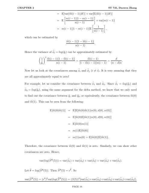
Now let us look at the covariances among � φi and � φj (i �= i). It is very amazing that they
are all approximately equal to zero!
For example, let us consider the covariance between � φ1 and � φ2. Since � φ1 = log(�q1) and
�φ2 = log(�q2), using the same argument for the delta method, we know that we only need
to find out the covariance between �q1 and �q2, or equivalently, the covariance between �m(0)
and �m(1). This can be seen from the following:
E[�m(0)�m(1)] = E[E[�m(0)�m(1)|n(0),d(0),w(0)]]
= E[�m(0)E[�m(1)|n(0),d(0),w(0)]]
= E[�m(0)m(1)]
= m(1)E[�m(0)]
= m(1)m(0) = E[�m(0)]E[�m(1)].
Therefore, the covariance between �m(0) and �m(1) is zero. Similarly, we can show other
covariances are zero. Hence,
var(log( � S R (5))) = var( � φ1)+var( � φ2)+var( � φ3)+var( � φ4)+var( � φ5).
Let � θ = log( � S R (5)). Then � S R (5) = e �θ .So
var( � S R (5)) = (e θ ) 2 var(log( � S R (5))) = (S(5)) 2 [var( � φ1)+var( � φ2)+var( � φ3)+var( � φ4)+var( � φ5)],
PAGE 16