ST 520 Statistical Principles of Clinical Trials - NCSU Statistics ...
ST 520 Statistical Principles of Clinical Trials - NCSU Statistics ...
ST 520 Statistical Principles of Clinical Trials - NCSU Statistics ...

You also want an ePaper? Increase the reach of your titles
YUMPU automatically turns print PDFs into web optimized ePapers that Google loves.
<strong>ST</strong> <strong>520</strong><br />
<strong>Statistical</strong> <strong>Principles</strong> <strong>of</strong> <strong>Clinical</strong> <strong>Trials</strong><br />
Lecture Notes<br />
(Modified from Dr. A. Tsiatis’ Lecture Notes)<br />
Daowen Zhang<br />
Department <strong>of</strong> <strong>Statistics</strong><br />
North Carolina State University<br />
c○2009 by Anastasios A. Tsiatis and Daowen Zhang
TABLE OF CONTENTS <strong>ST</strong> <strong>520</strong>, A. Tsiatis and D. Zhang<br />
Contents<br />
1 Introduction 1<br />
1.1 Scope and objectives . . . . . . . . . . . . . . . . . . . . . . . . . . . . . . . . . . 1<br />
1.2 Brief Introduction to Epidemiology . . . . . . . . . . . . . . . . . . . . . . . . . . 2<br />
1.3 Brief Introduction and History <strong>of</strong> <strong>Clinical</strong> <strong>Trials</strong> . . . . . . . . . . . . . . . . . . . 12<br />
2 Phase I and II clinical trials 18<br />
2.1 Phases <strong>of</strong> <strong>Clinical</strong> <strong>Trials</strong> . . . . . . . . . . . . . . . . . . . . . . . . . . . . . . . . 18<br />
2.2 Phase II clinical trials . . . . . . . . . . . . . . . . . . . . . . . . . . . . . . . . . 20<br />
2.2.1 <strong>Statistical</strong> Issues and Methods . . . . . . . . . . . . . . . . . . . . . . . . . 21<br />
2.2.2 Gehan’s Two-Stage Design . . . . . . . . . . . . . . . . . . . . . . . . . . . 28<br />
2.2.3 Simon’s Two-Stage Design . . . . . . . . . . . . . . . . . . . . . . . . . . . 29<br />
3 Phase III <strong>Clinical</strong> <strong>Trials</strong> 35<br />
3.1 Why are clinical trials needed . . . . . . . . . . . . . . . . . . . . . . . . . . . . . 35<br />
3.2 Issues to consider before designing a clinical trial . . . . . . . . . . . . . . . . . . 36<br />
3.3 Ethical Issues . . . . . . . . . . . . . . . . . . . . . . . . . . . . . . . . . . . . . . 39<br />
3.4 The Randomized <strong>Clinical</strong> Trial . . . . . . . . . . . . . . . . . . . . . . . . . . . . . 40<br />
3.5 Review <strong>of</strong> Conditional Expectation and Conditional Variance . . . . . . . . . . . . 43<br />
4 Randomization 49<br />
4.1 Design-based Inference . . . . . . . . . . . . . . . . . . . . . . . . . . . . . . . . . 49<br />
4.2 Fixed Allocation Randomization . . . . . . . . . . . . . . . . . . . . . . . . . . . . 53<br />
4.2.1 Simple Randomization . . . . . . . . . . . . . . . . . . . . . . . . . . . . . 56<br />
4.2.2 Permuted block randomization . . . . . . . . . . . . . . . . . . . . . . . . . 57<br />
4.2.3 Stratified Randomization . . . . . . . . . . . . . . . . . . . . . . . . . . . . 59<br />
4.3 Adaptive Randomization Procedures . . . . . . . . . . . . . . . . . . . . . . . . . 66<br />
4.3.1 Efron biased coin design . . . . . . . . . . . . . . . . . . . . . . . . . . . . 66<br />
4.3.2 Urn Model (L.J. Wei) . . . . . . . . . . . . . . . . . . . . . . . . . . . . . . 67<br />
4.3.3 Minimization Method <strong>of</strong> Pocock and Simon . . . . . . . . . . . . . . . . . 67<br />
i
TABLE OF CONTENTS <strong>ST</strong> <strong>520</strong>, A. Tsiatis and D. Zhang<br />
4.4 Response Adaptive Randomization . . . . . . . . . . . . . . . . . . . . . . . . . . 70<br />
4.5 Mechanics <strong>of</strong> Randomization . . . . . . . . . . . . . . . . . . . . . . . . . . . . . . 71<br />
5 Some Additional Issues in Phase III <strong>Clinical</strong> <strong>Trials</strong> 74<br />
5.1 Blinding and Placebos . . . . . . . . . . . . . . . . . . . . . . . . . . . . . . . . . 74<br />
5.2 Ethics . . . . . . . . . . . . . . . . . . . . . . . . . . . . . . . . . . . . . . . . . . 75<br />
5.3 The Protocol Document . . . . . . . . . . . . . . . . . . . . . . . . . . . . . . . . 77<br />
6 Sample Size Calculations 81<br />
6.1 Hypothesis Testing . . . . . . . . . . . . . . . . . . . . . . . . . . . . . . . . . . . 81<br />
6.2 Deriving sample size to achieve desired power . . . . . . . . . . . . . . . . . . . . 87<br />
6.3 Comparing two response rates . . . . . . . . . . . . . . . . . . . . . . . . . . . . . 88<br />
6.3.1 Arcsin square root transformation . . . . . . . . . . . . . . . . . . . . . . . 92<br />
7 Comparing More Than Two Treatments 96<br />
7.1 Testing equality using independent normally distributed estimators . . . . . . . . 97<br />
7.2 Testing equality <strong>of</strong> dichotomous response rates . . . . . . . . . . . . . . . . . . . . 98<br />
7.3 Multiple comparisons . . . . . . . . . . . . . . . . . . . . . . . . . . . . . . . . . . 102<br />
7.4 K-sample tests for continuous response . . . . . . . . . . . . . . . . . . . . . . . . 109<br />
7.5 Sample size computations for continuous response . . . . . . . . . . . . . . . . . . 112<br />
7.6 Equivalency <strong>Trials</strong> . . . . . . . . . . . . . . . . . . . . . . . . . . . . . . . . . . . 113<br />
8 Causality, Non-compliance and Intent-to-treat 118<br />
8.1 Causality and Counterfactual Random Variables . . . . . . . . . . . . . . . . . . . 118<br />
8.2 Noncompliance and Intent-to-treat analysis . . . . . . . . . . . . . . . . . . . . . . 122<br />
8.3 A Causal Model with Noncompliance . . . . . . . . . . . . . . . . . . . . . . . . . 124<br />
9 Survival Analysis in Phase III <strong>Clinical</strong> <strong>Trials</strong> 131<br />
9.1 Describing the Distribution <strong>of</strong> Time to Event . . . . . . . . . . . . . . . . . . . . . 132<br />
9.2 Censoring and Life-Table Methods . . . . . . . . . . . . . . . . . . . . . . . . . . 136<br />
9.3 Kaplan-Meier or Product-Limit Estimator . . . . . . . . . . . . . . . . . . . . . . 140<br />
ii
TABLE OF CONTENTS <strong>ST</strong> <strong>520</strong>, A. Tsiatis and D. Zhang<br />
9.4 Two-sample Tests . . . . . . . . . . . . . . . . . . . . . . . . . . . . . . . . . . . . 144<br />
9.5 Power and Sample Size . . . . . . . . . . . . . . . . . . . . . . . . . . . . . . . . . 149<br />
9.6 K-Sample Tests . . . . . . . . . . . . . . . . . . . . . . . . . . . . . . . . . . . . . 157<br />
9.7 Sample-size considerations for the K-sample logrank test . . . . . . . . . . . . . . 160<br />
10 Early Stopping <strong>of</strong> <strong>Clinical</strong> <strong>Trials</strong> 164<br />
10.1 General issues in monitoring clinical trials . . . . . . . . . . . . . . . . . . . . . . 164<br />
10.2 Information based design and monitoring . . . . . . . . . . . . . . . . . . . . . . . 167<br />
10.3 Type I error . . . . . . . . . . . . . . . . . . . . . . . . . . . . . . . . . . . . . . . 171<br />
10.3.1 Equal increments <strong>of</strong> information . . . . . . . . . . . . . . . . . . . . . . . . 175<br />
10.4 Choice <strong>of</strong> boundaries . . . . . . . . . . . . . . . . . . . . . . . . . . . . . . . . . . 177<br />
10.4.1 Pocock boundaries . . . . . . . . . . . . . . . . . . . . . . . . . . . . . . . 178<br />
10.4.2 O’Brien-Fleming boundaries . . . . . . . . . . . . . . . . . . . . . . . . . . 179<br />
10.5 Power and sample size in terms <strong>of</strong> information . . . . . . . . . . . . . . . . . . . . 181<br />
10.5.1 Inflation Factor . . . . . . . . . . . . . . . . . . . . . . . . . . . . . . . . . 184<br />
10.5.2 Information based monitoring . . . . . . . . . . . . . . . . . . . . . . . . . 188<br />
10.5.3 Average information . . . . . . . . . . . . . . . . . . . . . . . . . . . . . . 189<br />
10.5.4 Steps in the design and analysis <strong>of</strong> group-sequential tests with equal increments<br />
<strong>of</strong> information . . . . . . . . . . . . . . . . . . . . . . . . . . . . . . 193<br />
iii
CHAPTER 1 <strong>ST</strong> <strong>520</strong>, A. TSIATIS and D. Zhang<br />
1 Introduction<br />
1.1 Scope and objectives<br />
The focus <strong>of</strong> this course will be on the statistical methods and principles used to study disease<br />
and its prevention or treatment in human populations. There are two broad subject areas in<br />
the study <strong>of</strong> disease; Epidemiology and <strong>Clinical</strong> <strong>Trials</strong>. This course will be devoted almost<br />
entirely to statistical methods in <strong>Clinical</strong> <strong>Trials</strong> research but we will first give a very brief intro-<br />
duction to Epidemiology in this Section.<br />
EPIDEMIOLOGY: Systematic study <strong>of</strong> disease etiology (causes and origins <strong>of</strong> disease) us-<br />
ing observational data (i.e. data collected from a population not under a controlled experimental<br />
setting).<br />
• Second hand smoking and lung cancer<br />
• Air pollution and respiratory illness<br />
• Diet and Heart disease<br />
• Water contamination and childhood leukemia<br />
• Finding the prevalence and incidence <strong>of</strong> HIV infection and AIDS<br />
CLINICAL TRIALS: The evaluation <strong>of</strong> intervention (treatment) on disease in a controlled<br />
experimental setting.<br />
• The comparison <strong>of</strong> AZT versus no treatment on the length <strong>of</strong> survival in patients with<br />
AIDS<br />
• Evaluating the effectiveness <strong>of</strong> a new anti-fungal medication on Athlete’s foot<br />
• Evaluating hormonal therapy on the reduction <strong>of</strong> breast cancer (Womens Health Initiative)<br />
PAGE 1
CHAPTER 1 <strong>ST</strong> <strong>520</strong>, A. TSIATIS and D. Zhang<br />
1.2 Brief Introduction to Epidemiology<br />
Cross-sectional study<br />
In a cross-sectional study the data are obtained from a random sample <strong>of</strong> the population at one<br />
point in time. This gives a snapshot <strong>of</strong> a population.<br />
Example: Based on a single survey <strong>of</strong> a specific population or a random sample there<strong>of</strong>, we<br />
determine the proportion <strong>of</strong> individuals with heart disease at one point in time. This is referred to<br />
as the prevalence <strong>of</strong> disease. We may also collect demographic and other information which will<br />
allow us to break down prevalence broken by age, race, sex, socio-economic status, geographic,<br />
etc.<br />
Important public health information can be obtained this way which may be useful in determin-<br />
ing how to allocate health care resources. However such data are generally not very useful in<br />
determining causation.<br />
In an important special case where the exposure and disease are dichotomous, the data from a<br />
cross-sectional study can be represented as<br />
D ¯ D<br />
E n11 n12 n1+<br />
Ē n21 n22 n2+<br />
n+1 n+2 n++<br />
where E = exposed (to risk factor), Ē = unexposed; D = disease, ¯ D = no disease.<br />
In this case, all counts except n++, the sample size, are random variables. The counts<br />
(n11, n12, n21, n22) have the following distribution:<br />
(n11, n12, n21, n22) ∼ multinomial(n++, P[DE], P[ ¯ DE], P[D Ē], P[ ¯ D Ē]).<br />
With this study, we can obtain estimates <strong>of</strong> the following parameters <strong>of</strong> interest<br />
prevalence <strong>of</strong> disease P[D] (estimated by n+1<br />
)<br />
n++<br />
probability <strong>of</strong> exposure P[E] (estimated by n1+<br />
)<br />
PAGE 2<br />
n++
CHAPTER 1 <strong>ST</strong> <strong>520</strong>, A. TSIATIS and D. Zhang<br />
prevalence <strong>of</strong> disease among exposed P[D|E] (estimated by n11<br />
)<br />
n1+<br />
n21<br />
prevalence <strong>of</strong> disease among unexposed P[D| Ē] (estimated by )<br />
n2+<br />
...<br />
We can also assess the association between the exposure and disease using the data from a<br />
cross-sectional study. One such measure is relative risk, which is defined as<br />
ψ = P[D|E]<br />
P[D| Ē].<br />
It is easy to see that the relative risk ψ has the following properties:<br />
• ψ > 1 ⇒ positive association; that is, the exposed population has higher disease probability<br />
than the unexposed population.<br />
• ψ = 1 ⇒ no association; that is, the exposed population has the same disease probability<br />
as the unexposed population.<br />
• ψ < 1 ⇒ negative association; that is, the exposed population has lower disease probability<br />
than the unexposed population.<br />
Of course, we cannot state that the exposure E causes the disease D even if ψ > 1, or vice versa.<br />
In fact, the exposure E may not even occur before the event D.<br />
Since we got good estimates <strong>of</strong> P[D|E] and P[D| Ē]<br />
the relative risk ψ can be estimated by<br />
�P[D|E] = n11<br />
, P[D|Ē] � = n21<br />
,<br />
n1+<br />
�ψ = � P[D|E] n11/n1+<br />
�P[D|<br />
= .<br />
Ē] n21/n2+<br />
Another measure that describes the association between the exposure and the disease is the<br />
odds ratio, which is defined as<br />
θ =<br />
P[D|E]/(1 − P[D|E])<br />
P[D| Ē]/(1 − P[D|Ē]).<br />
Note that P[D|E]/(1 − P[D|E]) is called the odds <strong>of</strong> P[D|E]. It is obvious that<br />
PAGE 3<br />
n2+
CHAPTER 1 <strong>ST</strong> <strong>520</strong>, A. TSIATIS and D. Zhang<br />
• ψ > 1 ⇐⇒ θ > 1<br />
• ψ = 1 ⇐⇒ θ = 1<br />
• ψ < 1 ⇐⇒ θ < 1<br />
Given data from a cross-sectional study, the odds ratio θ can be estimated by<br />
�θ =<br />
�P[D|E]/(1 − � P[D|E])<br />
�P[D| Ē]/(1 − � P[D| Ē]) = n11/n1+/(1 − n11/n1+) n11/n12<br />
=<br />
n21/n2+/(1 − n21/n2+) n21/n22<br />
It can be shown that the variance <strong>of</strong> log( � θ) has a very nice form given by<br />
�var(log( � θ)) = 1<br />
n11<br />
+ 1<br />
+<br />
n12<br />
1<br />
+<br />
n21<br />
1<br />
.<br />
n22<br />
= n11n22<br />
.<br />
n12n21<br />
The point estimate � θ and the above variance estimate can be used to make inference on θ. Of<br />
course, the total sample size n++ as well as each cell count have to be large for this variance<br />
formula to be reasonably good.<br />
A (1 − α) confidence interval (CI) for log(θ) (log odds ratio) is<br />
log( � θ) ± zα/2[ � Var(log( � θ))] 1/2 .<br />
Exponentiating the two limits <strong>of</strong> the above interval will give us a CI for θ with the same confidence<br />
level (1 − α).<br />
Alternatively, the variance <strong>of</strong> � θ can be estimated (by the delta method)<br />
�Var( � θ) = � θ 2<br />
�<br />
1<br />
and a (1 − α) CI for θ is obtained as<br />
n11<br />
+ 1<br />
+<br />
n12<br />
1<br />
+<br />
n21<br />
1<br />
�<br />
,<br />
n22<br />
�θ ± zα/2[ � Var( � θ)] 1/2 .<br />
For example, if we want a 95% confidence interval for log(θ) or θ, we will use z0.05/2 = 1.96 in<br />
the above formulas.<br />
From the definition <strong>of</strong> the odds-ration, we see that if the disease under study is a rare one, then<br />
P[D|E] ≈ 0, P[D| Ē] ≈ 0.<br />
PAGE 4
CHAPTER 1 <strong>ST</strong> <strong>520</strong>, A. TSIATIS and D. Zhang<br />
In this case, we have<br />
θ ≈ ψ.<br />
This approximation is very useful. Since the relative risk ψ has a much better interpretation<br />
(and hence it is easier to communicate with biomedical researchers using this measure), in stud-<br />
ies where we cannot estimate the relative risk ψ but we can estimate the odds-ratio θ (see<br />
retrospective studies later), if the disease under studied is a rare one, we can approximately<br />
estimate the relative risk by the odds-ratio estimate.<br />
Longitudinal studies<br />
In a longitudinal study, subjects are followed over time and single or multiple measurements <strong>of</strong><br />
the variables <strong>of</strong> interest are obtained. Longitudinal epidemiological studies generally fall into<br />
two categories; prospective i.e. moving forward in time or retrospective going backward in<br />
time. We will focus on the case where a single measurement is taken.<br />
Prospective study: In a prospective study, a cohort <strong>of</strong> individuals are identified who are free<br />
<strong>of</strong> a particular disease under study and data are collected on certain risk factors; i.e. smoking<br />
status, drinking status, exposure to contaminants, age, sex, race, etc. These individuals are<br />
then followed over some specified period <strong>of</strong> time to determine whether they get disease or not.<br />
The relationships between the probability <strong>of</strong> getting disease during a certain time period (called<br />
incidence <strong>of</strong> the disease) and the risk factors are then examined.<br />
If there is only one exposure variable which is binary, the data from a prospective study may be<br />
summarized as<br />
D ¯ D<br />
E n11 n12 n1+<br />
Ē n21 n22 n2+<br />
Since the cohorts are identified by the researcher, n1+ and n2+ are fixed sample sizes for each<br />
group. In this case, only n11 and n21 are random variables, and these random variables have the<br />
PAGE 5
CHAPTER 1 <strong>ST</strong> <strong>520</strong>, A. TSIATIS and D. Zhang<br />
following distributions:<br />
n11 ∼ Bin(n1+, P[D|E]), n21 ∼ Bin(n2+, P[D| Ē]).<br />
From these distributions, P[D|E]) and P[D| Ē] can be readily estimated by<br />
�P[D|E] = n11<br />
, P[D|Ē] � = n21<br />
.<br />
n1+<br />
The relative risk ψ and the odds-ratio θ defined previously can be estimated in exactly the same<br />
way (have the same formula). So does the variance estimate <strong>of</strong> the odds-ratio estimate.<br />
One problem <strong>of</strong> a prospective study is that some subjects may drop out from the study before<br />
developing the disease under study. In this case, the disease probability has to be estimated<br />
differently. This is illustrated by the following example.<br />
Example: 40,000 British doctors were followed for 10 years. The following data were collected:<br />
n2+<br />
Table 1.1: Death Rate from Lung Cancer per 1000 person years.<br />
# cigarettes smoked per day death rate<br />
0 .07<br />
1-14 .57<br />
15-24 1.39<br />
35+ 2.27<br />
For presentation purpose, the estimated rates are multiplied by 1000.<br />
Remark: If we denote by T the time to death due to lung cancer, the death rate at time t is<br />
defined by<br />
λ(t) = lim<br />
h→0<br />
P[t ≤ T < t + h|T ≥ t]<br />
.<br />
h<br />
Assume the death rate λ(t) is a constant λ, then it can be estimated by<br />
�λ =<br />
total number <strong>of</strong> deaths from lunge cancer<br />
total person years <strong>of</strong> exposure (smoking) during the 10 year period .<br />
In this case, if we are interested in the event<br />
D = die from lung cancer within next one year | still alive now,<br />
PAGE 6
CHAPTER 1 <strong>ST</strong> <strong>520</strong>, A. TSIATIS and D. Zhang<br />
or statistically,<br />
then<br />
D = [t ≤ T < t + 1|T ≥ t],<br />
P[D] = P[t ≤ T ≤ t + 1|T ≥ t] = 1 − e −λ ≈ λ, if λ is very small.<br />
Roughly speaking, assuming the death rate remains constant over the 10 year period for each<br />
group <strong>of</strong> doctors, we can take the rate above divided by 1000 to approximate the probability <strong>of</strong><br />
death from lung cancer in one year. For example, the estimated probability <strong>of</strong> dying from lung<br />
cancer in one year for British doctors smoking between 15-24 cigarettes per day at the beginning<br />
<strong>of</strong> the study is � P[D] = 1.39/1000 = 0.00139. Similarly, the estimated probability <strong>of</strong> dying from<br />
lung cancer in one year for the heaviest smokers is � P[D] = 2.27/1000 = 0.00227.<br />
From the table above we note that the relative risk <strong>of</strong> death from lung cancer between heavy<br />
smokers and non-smokers (in the same time window) is 2.27/0.07 = 32.43. That is, heavy smokers<br />
are estimated to have 32 times the risk <strong>of</strong> dying from lung cancer as compared to non-smokers.<br />
Certainly the value 32 is subject to statistical variability and moreover we must be concerned<br />
whether these results imply causality.<br />
We can also estimate the odds-ratio <strong>of</strong> dying from lung cancer in one year between heavy smokers<br />
and non-smokers:<br />
�θ =<br />
.00227/(1 − .00227)<br />
= 32.50.<br />
.00007/(1 − .00007)<br />
This estimate is essentially the same as the estimate <strong>of</strong> the relative risk 32.43.<br />
Retrospective study: Case-Control<br />
A very popular design in many epidemiological studies is the case-control design. In such a<br />
study individuals with disease (called cases) and individuals without disease (called controls)<br />
are identified. Using records or questionnaires the investigators go back in time and ascertain<br />
exposure status and risk factors from their past. Such data are used to estimate relative risk as<br />
we will demonstrate.<br />
Example: A sample <strong>of</strong> 1357 male patients with lung cancer (cases) and a sample <strong>of</strong> 1357 males<br />
without lung cancer (controls) were surveyed about their past smoking history. This resulted in<br />
PAGE 7
CHAPTER 1 <strong>ST</strong> <strong>520</strong>, A. TSIATIS and D. Zhang<br />
the following:<br />
smoke cases controls<br />
yes 1,289 921<br />
no 68 436<br />
We would like to estimate the relative risk ψ or the odds-ratio θ <strong>of</strong> getting lung cancer between<br />
smokers and non-smokers.<br />
Before tackling this problem, let us look at a general problem. The above data can be represented<br />
by the following 2 × 2 table:<br />
D ¯ D<br />
E n11 n12<br />
Ē n21 n22<br />
n+1 n+2<br />
By the study design, the margins n+1 and n+2 are fixed numbers, and the counts n11 and n12 are<br />
random variables having the following distributions:<br />
By definition, the relative risk ψ is<br />
n11 ∼ Bin(n+1, P[E|D]), n12 ∼ Bin(n+2, P[E| ¯ D]).<br />
ψ = P[D|E]<br />
P[D| Ē].<br />
We can estimate ψ if we can estimate these probabilities P[D|E] and P[D| Ē]. However, we<br />
cannot use the same formulas we used before for cross-sectional or prospective study to estimate<br />
them.<br />
What is the consequence <strong>of</strong> using the same formulas we used before? The formulas would lead<br />
to the following incorrect estimates:<br />
�P[D|E] = n11<br />
n1+<br />
n21<br />
�P[D| Ē] =<br />
n2+<br />
=<br />
=<br />
n11<br />
n11 + n12<br />
n21<br />
n21 + n22<br />
PAGE 8<br />
(incorrect!)<br />
(incorrect!)
CHAPTER 1 <strong>ST</strong> <strong>520</strong>, A. TSIATIS and D. Zhang<br />
Since we choose n+1 and n+2, we can fix n+2 at some number (say, 50), and let n+1 grow (sample<br />
more cases). As long as P[E|D] > 0, n11 will also grow. Then � P[D|E] −→ 1. Similarly<br />
�P[D| Ē] −→ 1. Obviously, these are NOT sensible estimates.<br />
For example, if we used the above formulas for our example, we would get:<br />
�P[D|E]<br />
1289<br />
= = 0.583 (incorrect!)<br />
1289 + 921<br />
�P[D|<br />
68<br />
Ē] = = 0.135 (incorrect!)<br />
68 + 436<br />
�ψ = � P[D|E] 0.583<br />
�P[D|<br />
= = 4.32 (incorrect!).<br />
Ē] 0.135<br />
This incorrect estimate <strong>of</strong> the relative risk will be contrasted with the estimate from the correct<br />
method.<br />
We introduced the odds-ratio before to assess the association between the exposure (E) and the<br />
disease (D) as follows:<br />
θ =<br />
P[D|E]/(1 − P[D|E])<br />
P[D| Ē]/(1 − P[D|Ē])<br />
and we stated that if the disease under study is a rare one, then<br />
θ ≈ ψ.<br />
Since we cannot directly estimate the relative risk ψ from a retrospective (case-control) study<br />
due to its design feature, let us try to estimate the odds-ratio θ.<br />
For this purpose, we would like to establish the following equivalence:<br />
P[D|E]/(1 − P[D|E])<br />
θ =<br />
P[D| Ē]/(1 − P[D|Ē])<br />
= P[D|E]/P[ ¯ D|E]<br />
P[D| Ē]/P[ ¯ D| Ē]<br />
= P[D|E]/P[D|Ē]<br />
P[ ¯ D|E]/P[ ¯ D| Ē].<br />
By Bayes’ theorem, we have for any two events A and B<br />
P[A|B] = P[AB]<br />
P[B]<br />
PAGE 9<br />
P[B|A]P[A]<br />
= .<br />
P[B]
CHAPTER 1 <strong>ST</strong> <strong>520</strong>, A. TSIATIS and D. Zhang<br />
Therefore,<br />
and<br />
P[D|E] P[E|D]P[D]/P[E] P[E|D]/P[E]<br />
= =<br />
P[D| Ē] P[ Ē|D]P[D]/P[Ē] P[ Ē|D]/P[Ē]<br />
P[ ¯ D|E]<br />
P[ ¯ D| Ē] = P[E| ¯ D]P[ ¯ D]/P[E]<br />
P[ Ē| ¯ D]P[ ¯ D]/P[ Ē] = P[E| ¯ D]/P[E]<br />
P[ Ē| ¯ D]/P[ Ē],<br />
θ = P[D|E]/P[D|Ē]<br />
P[ ¯ D|E]/P[ ¯ D| Ē]<br />
= P[E|D]/P[Ē|D]<br />
P[E| ¯ D]/P[ Ē| ¯ D]<br />
= P[E|D]/(1 − P[E|D])<br />
P[E| ¯ D]/(1 − P[E| ¯ D]) .<br />
Notice that the quantity in the right hand side is in fact the odds-ratio <strong>of</strong> being exposed between<br />
cases and controls, and the above identity says that the odds-ratio <strong>of</strong> getting disease between<br />
exposed and un-exposed is the same as the odds-ratio <strong>of</strong> being exposed between cases and<br />
controls. This identity is very important since by design we are able to estimate the odds-ratio<br />
<strong>of</strong> being exposed between cases and controls since we are able to estimate P[E|D] and E| ¯ D] from<br />
a case-control study:<br />
So θ can be estimated by<br />
�P[E|D] = n11 n12<br />
, P[E| � D] ¯ = .<br />
n+1<br />
n+2<br />
�θ = � P[E|D]/(1 − � P[E|D])<br />
�P[E| ¯ D]/(1 − � P[E| ¯ D]) = n11/n+1/(1 − n11/n+1) n11/n21<br />
=<br />
n12/n+2/(1 − n12/n+2) n12/n22<br />
= n11n22<br />
,<br />
n12n21<br />
which has exactly the same form as the estimate from a cross-sectional or prospective study.<br />
This means that the odds-ratio estimate is invariant to the study design.<br />
Similarly, it can be shown that the variance <strong>of</strong> log( � θ) can be estimated by the same formula we<br />
used before<br />
�Var(log( � θ)) = 1<br />
n11<br />
+ 1<br />
+<br />
n12<br />
1<br />
+<br />
n21<br />
1<br />
.<br />
n22<br />
Therefore, inference on θ or log(θ) such as constructing a confidence interval will be exactly the<br />
same as before.<br />
Going back to the lung cancer example, we got the following estimate <strong>of</strong> the odds ratio:<br />
�θ =<br />
1289 × 436<br />
921 × 68<br />
PAGE 10<br />
= 8.97.
CHAPTER 1 <strong>ST</strong> <strong>520</strong>, A. TSIATIS and D. Zhang<br />
If lung cancer can be viewed as a rare event, we estimate the relative risk <strong>of</strong> getting lung cancer<br />
between smokers and non-smokers to be about nine fold. This estimate is much higher than the<br />
incorrect estimate (4.32) we got on page 9.<br />
Pros and Cons <strong>of</strong> a case-control study<br />
• Pros<br />
• Cons<br />
– Can be done more quickly. You don’t have to wait for the disease to appear over time.<br />
– If the disease is rare, a case-control design can give a more precise estimate <strong>of</strong> relative<br />
risk with the same number <strong>of</strong> patients than a prospective design. This is because the<br />
number <strong>of</strong> cases, which in a prospective study is small, would be over-represented by<br />
design in a case control study. This will be illustrated in a homework exercise.<br />
– It may be difficult to get accurate information on the exposure status <strong>of</strong> cases and<br />
controls. The records may not be that good and depending on individuals’ memory<br />
may not be very reliable. This can be a severe drawback.<br />
PAGE 11
CHAPTER 1 <strong>ST</strong> <strong>520</strong>, A. TSIATIS and D. Zhang<br />
1.3 Brief Introduction and History <strong>of</strong> <strong>Clinical</strong> <strong>Trials</strong><br />
The following are several definitions <strong>of</strong> a clinical trial that were found in different textbooks and<br />
articles.<br />
• A clinical trial is a study in human subjects in which treatment (intervention) is initiated<br />
specifically for therapy evaluation.<br />
• A prospective study comparing the effect and value <strong>of</strong> intervention against a control in<br />
human beings.<br />
• A clinical trial is an experiment which involves patients and is designed to elucidate the<br />
most appropriate treatment <strong>of</strong> future patients.<br />
• A clinical trial is an experiment testing medical treatments in human subjects.<br />
Historical perspective<br />
Historically, the quantum unit <strong>of</strong> clinical reasoning has been the case history and the primary<br />
focus <strong>of</strong> clinical inference has been the individual patient. Inference from the individual to the<br />
population was informal. The advent <strong>of</strong> formal experimental methods and statistical reasoning<br />
made this process rigorous.<br />
By statistical reasoning or inference we mean the use <strong>of</strong> results on a limited sample <strong>of</strong> patients to<br />
infer how treatment should be administered in the general population who will require treatment<br />
in the future.<br />
Early History<br />
1600 East India Company<br />
In the first voyage <strong>of</strong> four ships– only one ship was provided with lemon juice. This was the only<br />
ship relatively free <strong>of</strong> scurvy.<br />
Note: This is observational data and a simple example <strong>of</strong> an epidemiological study.<br />
PAGE 12
CHAPTER 1 <strong>ST</strong> <strong>520</strong>, A. TSIATIS and D. Zhang<br />
1753 James Lind<br />
“I took 12 patients in the scurvy aboard the Salisbury at sea. The cases were as similar as I<br />
could have them... they lay together in one place... and had one common diet to them all...<br />
To two <strong>of</strong> them was given a quart <strong>of</strong> cider a day, to two an elixir <strong>of</strong> vitriol, to two vinegar, to<br />
two oranges and lemons, to two a course <strong>of</strong> sea water, and to the remaining two the bigness <strong>of</strong><br />
a nutmeg. The most sudden and visible good effects were perceived from the use <strong>of</strong> oranges and<br />
lemons, one <strong>of</strong> those who had taken them being at the end <strong>of</strong> six days fit for duty... and the<br />
other appointed nurse to the sick...<br />
Note: This is an example <strong>of</strong> a controlled clinical trial.<br />
Interestingly, although the trial appeared conclusive, Lind continued to propose “pure dry air” as<br />
the first priority with fruit and vegetables as a secondary recommendation. Furthermore, almost<br />
50 years elapsed before the British navy supplied lemon juice to its ships.<br />
Pre-20th century medical experimenters had no appreciation <strong>of</strong> the scientific method. A common<br />
medical treatment before 1800 was blood letting. It was believed that you could get rid <strong>of</strong> an<br />
ailment or infection by sucking the bad blood out <strong>of</strong> sick patients; usually this was accomplished<br />
by applying leeches to the body. There were numerous anecdotal accounts <strong>of</strong> the effectiveness <strong>of</strong><br />
such treatment for a myriad <strong>of</strong> diseases. The notion <strong>of</strong> systematically collecting data to address<br />
specific issues was quite foreign.<br />
1794 Rush Treatment <strong>of</strong> yellow fever by bleeding<br />
“I began by drawing a small quantity at a time. The appearance <strong>of</strong> the blood and its effects upon<br />
the system satisfied me <strong>of</strong> its safety and efficacy. Never before did I experience such sublime joy<br />
as I now felt in contemplating the success <strong>of</strong> my remedies... The reader will not wonder when I<br />
add a short extract from my notebook, dated 10th September. “Thank God”, <strong>of</strong> the one hundred<br />
patients, whom I visited, or prescribed for, this day, I have lost none.”<br />
Louis (1834): Lays a clear foundation for the use <strong>of</strong> the numerical method in assessing therapies.<br />
“As to different methods <strong>of</strong> treatment, if it is possible for us to assure ourselves <strong>of</strong> the superiority<br />
<strong>of</strong> one or other among them in any disease whatever, having regard to the different circumstances<br />
PAGE 13
CHAPTER 1 <strong>ST</strong> <strong>520</strong>, A. TSIATIS and D. Zhang<br />
Table 1.2: Pneumonia: Effects <strong>of</strong> Blood Letting<br />
Days bled proportion<br />
after onset Died Lived surviving<br />
1-3 12 12 50%<br />
4-6 12 22 65%<br />
7-9 3 16 84%<br />
<strong>of</strong> age, sex and temperament, <strong>of</strong> strength and weakness, it is doubtless to be done by enquiring<br />
if under these circumstances a greater number <strong>of</strong> individuals have been cured by one means than<br />
another. Here again it is necessary to count. And it is, in great part at least, because hitherto<br />
this method has been not at all, or rarely employed, that the science <strong>of</strong> therapeutics is still so<br />
uncertain; that when the application <strong>of</strong> the means placed in our hands is useful we do not know<br />
the bounds <strong>of</strong> this utility.”<br />
He goes on to discuss the need for<br />
• The exact observation <strong>of</strong> patient outcome<br />
• Knowledge <strong>of</strong> the natural progress <strong>of</strong> untreated controls<br />
• Precise definition <strong>of</strong> disease prior to treatment<br />
• Careful observations <strong>of</strong> deviations from intended treatment<br />
Louis (1835) studied the value <strong>of</strong> bleeding as a treatment <strong>of</strong> pneumonia, erysipelas and throat<br />
inflammation and found no demonstrable difference in patients bled and not bled. This finding<br />
contradicted current clinical practice in France and instigated the eventual decline in bleeding<br />
as a standard treatment. Louis had an immense influence on clinical practice in France, Britain<br />
and America and can be considered the founding figure who established clinical trials and epi-<br />
demiology on a scientific footing.<br />
In 1827: 33,000,000 leeches were imported to Paris.<br />
In 1837: 7,000 leeches were imported to Paris.<br />
PAGE 14
CHAPTER 1 <strong>ST</strong> <strong>520</strong>, A. TSIATIS and D. Zhang<br />
Modern clinical trials<br />
The first clinical trial with a properly randomized control group was set up to study streptomycin<br />
in the treatment <strong>of</strong> pulmonary tuberculosis, sponsored by the Medical Research Council, 1948.<br />
This was a multi-center clinical trial where patients were randomly allocated to streptomycin +<br />
bed rest versus bed rest alone.<br />
The evaluation <strong>of</strong> patient x-ray films was made independently by two radiologists and a clinician,<br />
each <strong>of</strong> whom did not know the others evaluations or which treatment the patient was given.<br />
Both patient survival and radiological improvement were significantly better on streptomycin.<br />
The field trial <strong>of</strong> the Salk Polio Vaccine<br />
In 1954, 1.8 million children participated in the largest trial ever to assess the effectiveness <strong>of</strong><br />
the Salk vaccine in preventing paralysis or death from poliomyelitis.<br />
Such a large number was needed because the incidence rate <strong>of</strong> polio was about 1 per 2,000 and<br />
evidence <strong>of</strong> treatment effect was needed as soon as possible so that vaccine could be routinely<br />
given if found to be efficacious.<br />
There were two components (randomized and non-randomized) to this trial. For the non-<br />
randomized component, one million children in the first through third grades participated. The<br />
second graders were <strong>of</strong>fered vaccine whereas first and third graders formed the control group.<br />
There was also a randomized component where .8 million children were randomized in a double-<br />
blind placebo-controlled trial.<br />
The incidence <strong>of</strong> polio in the randomized vaccinated group was less than half that in the control<br />
group and even larger differences were seen in the decline <strong>of</strong> paralytic polio.<br />
The nonrandomized group supported these results; however non-participation by some who were<br />
<strong>of</strong>fered vaccination might have cast doubt on the results. It turned out that the incidence <strong>of</strong> polio<br />
among children (second graders) <strong>of</strong>fered vaccine and not taking it (non-compliers) was different<br />
than those in the control group (first and third graders). This may cast doubt whether first and<br />
third graders (control group) have the same likelihood for getting polio as second graders. This is<br />
PAGE 15
CHAPTER 1 <strong>ST</strong> <strong>520</strong>, A. TSIATIS and D. Zhang<br />
a basic assumption that needs to be satisfied in order to make unbiased treatment comparisons.<br />
Luckily, there was a randomized component to the study where the two groups (vaccinated)<br />
versus (control) were guaranteed to be similar on average by design.<br />
Note: During the course <strong>of</strong> the semester there will be a great deal <strong>of</strong> discussion on the role <strong>of</strong><br />
randomization and compliance and their effect on making causal statements.<br />
Government sponsored studies<br />
In the 1950’s the National Cancer Institute (NCI) organized randomized clinical trials in acute<br />
leukemia. The successful organization <strong>of</strong> this particular clinical trial led to the formation <strong>of</strong> two<br />
collaborative groups; CALGB (Cancer and Leukemia Group B) and ECOG (Eastern Cooperative<br />
Oncology Group). More recently SWOG (Southwest Oncology Group) and POG (Pediatrics<br />
Oncology Group) have been organized. A Cooperative group is an organization with many<br />
participating hospitals throughout the country (sometimes world) that agree to conduct common<br />
clinical trials to assess treatments in different disease areas.<br />
Government sponsored clinical trials are now routine. As well as the NCI, these include the<br />
following organizations <strong>of</strong> the National Institutes <strong>of</strong> Health.<br />
• NHLBI- (National Heart Lung and Blood Institute) funds individual and <strong>of</strong>ten very large<br />
studies in heart disease. To the best <strong>of</strong> my knowledge there are no cooperative groups<br />
funded by NHLBI.<br />
• NIAID- (National Institute <strong>of</strong> Allergic and Infectious Diseases) Much <strong>of</strong> their funding now<br />
goes to clinical trials research for patients with HIV and AIDS. The ACTG (AIDS <strong>Clinical</strong><br />
<strong>Trials</strong> Group) is a large cooperative group funded by NIAID.<br />
• NIDDK- (National Institute <strong>of</strong> Diabetes and Digestive and Kidney Diseases). Funds large<br />
scale clinical trials in diabetes research. Recently formed the cooperative group TRIALNET<br />
(network 18 clinical centers working in cooperation with screening sites throughout the<br />
United States, Canada, Finland, United Kingdom, Italy, Germany, Australia, and New<br />
Zealand - for type 1 diabetes)<br />
PAGE 16
CHAPTER 1 <strong>ST</strong> <strong>520</strong>, A. TSIATIS and D. Zhang<br />
Pharmaceutical Industry<br />
• Before World War II no formal requirements were made for conducting clinical trials before<br />
a drug could be freely marketed.<br />
• In 1938, animal research was necessary to document toxicity, otherwise human data could<br />
be mostly anecdotal.<br />
• In 1962, it was required that an “adequate and well controlled trial” be conducted.<br />
• In 1969, it became mandatory that evidence from a randomized clinical trial was necessary<br />
to get marketing approval from the Food and Drug Administration (FDA).<br />
• More recently there is effort in standardizing the process <strong>of</strong> drug approval worldwide. This<br />
has been through efforts <strong>of</strong> the International Conference on Harmonization (ICH).<br />
website: http://www.pharmweb.net/pwmirror/pw9/ifpma/ich1.html<br />
• There are more clinical trials currently taking place than ever before. The great majority<br />
<strong>of</strong> the clinical trial effort is supported by the Pharmaceutical Industry for the evaluation<br />
and marketing <strong>of</strong> new drug treatments. Because the evaluation <strong>of</strong> drugs and the conduct,<br />
design and analysis <strong>of</strong> clinical trials depends so heavily on sound <strong>Statistical</strong> Methodology<br />
this has resulted in an explosion <strong>of</strong> statisticians working for th Pharmaceutical Industry<br />
and wonderful career opportunities.<br />
PAGE 17
CHAPTER 2 <strong>ST</strong> <strong>520</strong>, A. TSIATIS and D. Zhang<br />
2 Phase I and II clinical trials<br />
2.1 Phases <strong>of</strong> <strong>Clinical</strong> <strong>Trials</strong><br />
The process <strong>of</strong> drug development can be broadly classified as pre-clinical and clinical. Pre-<br />
clinical refers to experimentation that occurs before it is given to human subjects; whereas,<br />
clinical refers to experimentation with humans. This course will consider only clinical research.<br />
It will be assumed that the drug has already been developed by the chemist or biologist, tested<br />
in the laboratory for biologic activity (in vitro), that preliminary tests on animals have been<br />
conducted (in vivo) and that the new drug or therapy is found to be sufficiently promising to be<br />
introduced into humans.<br />
Within the realm <strong>of</strong> clinical research, clinical trials are classified into four phases.<br />
• Phase I: To explore possible toxic effects <strong>of</strong> drugs and determine a tolerated dose for<br />
further experimentation. Also during Phase I experimentation the pharmacology <strong>of</strong> the<br />
drug may be explored.<br />
• Phase II: Screening and feasibility by initial assessment for therapeutic effects; further<br />
assessment <strong>of</strong> toxicities.<br />
• Phase III: Comparison <strong>of</strong> new intervention (drug or therapy) to the current standard <strong>of</strong><br />
treatment; both with respect to efficacy and toxicity.<br />
• Phase IV: (post marketing) Observational study <strong>of</strong> morbidity/adverse effects.<br />
These definitions <strong>of</strong> the four phases are not hard and fast. Many clinical trials blur the lines<br />
between the phases. Loosely speaking, the logic behind the four phases is as follows:<br />
A new promising drug is about to be assessed in humans. The effect that this drug might have<br />
on humans is unknown. We might have some experience on similar acting drugs developed in<br />
the past and we may also have some data on the effect this drug has on animals but we are not<br />
sure what the effect is on humans. To study the initial effects, a Phase I study is conducted.<br />
Using increasing doses <strong>of</strong> the drug on a small number <strong>of</strong> subjects, the possible side effects <strong>of</strong> the<br />
drug are documented. It is during this phase that the tolerated dose is determined for future<br />
PAGE 18
CHAPTER 2 <strong>ST</strong> <strong>520</strong>, A. TSIATIS and D. Zhang<br />
experimentation. The general dogma is that the therapeutic effect <strong>of</strong> the drug will increase with<br />
dose, but also the toxic effects will increase as well. Therefore one <strong>of</strong> the goals <strong>of</strong> a Phase I study<br />
is to determine what the maximum dose should be that can be reasonably tolerated by most<br />
individuals with the disease. The determination <strong>of</strong> this dose is important as this will be used in<br />
future studies when determining the effectiveness <strong>of</strong> the drug. If we are too conservative then we<br />
may not be giving enough drug to get the full therapeutic effect. On the other hand if we give<br />
too high a dose then people will have adverse effects and not be able to tolerate the drug.<br />
Once it is determined that a new drug can be tolerated and a dose has been established, the<br />
focus turns to whether the drug is good. Before launching into a costly large-scale comparison<br />
<strong>of</strong> the new drug to the current standard treatment, a smaller feasibility study is conducted to<br />
assess whether there is sufficient efficacy (activity <strong>of</strong> the drug on disease) to warrant further<br />
investigation. This occurs during phase II where drugs which show little promise are screened<br />
out.<br />
If the new drug still looks promising after phase II investigation it moves to Phase III testing<br />
where a comparison is made to a current standard treatment. These studies are generally large<br />
enough so that important treatment differences can be detected with sufficiently large probability.<br />
These studies are conducted carefully using sound statistical principles <strong>of</strong> experimental design<br />
established for clinical trials to make objective and unbiased comparisons. It is on the basis <strong>of</strong><br />
such Phase III clinical trials that new drugs are approved by regulatory agencies (such as FDA)<br />
for the general population <strong>of</strong> individuals with the disease for which this drug is targeted.<br />
Once a drug is on the market and a large number <strong>of</strong> patients are taking it, there is always the<br />
possibility <strong>of</strong> rare but serious side effects that can only be detected when a large number are<br />
given treatment for sufficiently long periods <strong>of</strong> time. It is important that a monitoring system<br />
be in place that allows such problems, if they occur, to be identified. This is the role <strong>of</strong> Phase<br />
IV studies.<br />
A brief discussion <strong>of</strong> phase I studies and designs and Pharmacology studies will be given based<br />
on the slides from Pr<strong>of</strong>essor Marie Davidian, an expert in pharmacokinetics. Slides on phase I<br />
and pharmacology will be posted on the course web page.<br />
PAGE 19
CHAPTER 2 <strong>ST</strong> <strong>520</strong>, A. TSIATIS and D. Zhang<br />
2.2 Phase II clinical trials<br />
After a new drug is tested in phase I for safety and tolerability, a dose finding study is sometimes<br />
conducted in phase II to identify a lowest dose level with good efficacy (close to the maximum<br />
efficacy achievable at tolerable dose level). In other situations, a phase II clinical trial uses a<br />
fixed dose chosen on the basis <strong>of</strong> a phase I clinical trial. The total dose is either fixed or may<br />
vary depending on the weight <strong>of</strong> the patient. There may also be provisions for modification <strong>of</strong><br />
the dose if toxicity occurs. The study population are patients with a specified disease for which<br />
the treatment is targeted.<br />
The primary objective is to determine whether the new treatment should be used in a large-scale<br />
comparative study. Phase II trials are used to assess<br />
• feasibility <strong>of</strong> treatment<br />
• side effects and toxicity<br />
• logistics <strong>of</strong> administration and cost<br />
The major issue that is addressed in a phase II clinical trial is whether there is enough evidence<br />
<strong>of</strong> efficacy to make it worth further study in a larger and more costly clinical trial. In a sense this<br />
is an initial screening tool for efficacy. During phase II experimentation the treatment efficacy<br />
is <strong>of</strong>ten evaluated on surrogate markers; i.e on an outcome that can be measured quickly and<br />
is believed to be related to the clinical outcome.<br />
Example: Suppose a new drug is developed for patients with lung cancer. Ultimately, we<br />
would like to know whether this drug will extend the life <strong>of</strong> lung cancer patients as compared to<br />
currently available treatments. Establishing the effect <strong>of</strong> a new drug on survival would require a<br />
long study with relatively large number <strong>of</strong> patients and thus may not be suitable as a screening<br />
mechanism. Instead, during phase II, the effect <strong>of</strong> the new drug may be assessed based on tumor<br />
shrinkage in the first few weeks <strong>of</strong> treatment. If the new drug shrinks tumors sufficiently for a<br />
sufficiently large proportion <strong>of</strong> patients, then this may be used as evidence for further testing.<br />
In this example, tumor shrinkage is a surrogate marker for overall survival time. The belief is<br />
that if the drug has no effect on tumor shrinkage it is unlikely to have an effect on the patient’s<br />
PAGE 20
CHAPTER 2 <strong>ST</strong> <strong>520</strong>, A. TSIATIS and D. Zhang<br />
overall survival and hence should be eliminated from further consideration. Unfortunately, there<br />
are many instances where a drug has a short term effect on a surrogate endpoint but ultimately<br />
may not have the long term effect on the clinical endpoint <strong>of</strong> ultimate interest. Furthermore,<br />
sometimes a drug may have beneficial effect through a biological mechanism that is not detected<br />
by the surrogate endpoint. Nonetheless, there must be some attempt at limiting the number <strong>of</strong><br />
drugs that will be considered for further testing or else the system would be overwhelmed.<br />
Other examples <strong>of</strong> surrogate markers are<br />
• Lowering blood pressure or cholesterol for patients with heart disease<br />
• Increasing CD4 counts or decreasing viral load for patients with HIV disease<br />
Most <strong>of</strong>ten, phase II clinical trials do not employ formal comparative designs. That is, they do<br />
not use parallel treatment groups. Often, phase II designs employ more than one stage; i.e. one<br />
group <strong>of</strong> patients are given treatment; if no (or little) evidence <strong>of</strong> efficacy is observed, then the<br />
trial is stopped and the drug is declared a failure; otherwise, more patients are entered in the<br />
next stage after which a final decision is made whether to move the drug forward or not.<br />
2.2.1 <strong>Statistical</strong> Issues and Methods<br />
One goal <strong>of</strong> a phase II trial is to estimate an endpoint related to treatment efficacy with sufficient<br />
precision to aid the investigators in determining whether the proposed treatment should be<br />
studied further.<br />
Some examples <strong>of</strong> endpoints are:<br />
• proportion <strong>of</strong> patients responding to treatment (response has to be unambiguously defined)<br />
• proportion with side effects<br />
• average decrease in blood pressure over a two week period<br />
A statistical perspective is generally taken for estimation and assessment <strong>of</strong> precision. That<br />
is, the problem is <strong>of</strong>ten posed through a statistical model with population parameters to be<br />
estimated and confidence intervals for these parameters to assess precision.<br />
PAGE 21
CHAPTER 2 <strong>ST</strong> <strong>520</strong>, A. TSIATIS and D. Zhang<br />
Example: Suppose we consider patients with esophogeal cancer treated with chemotherapy prior<br />
to surgical resection. A complete response is defined as an absence <strong>of</strong> macroscopic or microscopic<br />
tumor at the time <strong>of</strong> surgery. We suspect that this may occur with 35% (guess) probability using<br />
a drug under investigation in a phase II study. The 35% is just a guess, possibly based on similar<br />
acting drugs used in the past, and the goal is to estimate the actual response rate with sufficient<br />
precision, in this case we want the 95% confidence interval to be within 15% <strong>of</strong> the truth.<br />
As statisticians, we view the world as follows: We start by positing a statistical model; that is,<br />
let π denote the population complete response rate. We conduct an experiment: n patients with<br />
esophogeal cancer are treated with the chemotherapy prior to surgical resection and we collect<br />
data: the number <strong>of</strong> patients who have a complete response.<br />
The result <strong>of</strong> this experiment yields a random variable X, the number <strong>of</strong> patients in a sample <strong>of</strong><br />
size n that have a complete response. A popular model for this scenario is to assume that<br />
X ∼ binomial(n, π);<br />
that is, the random variable X is distributed with a binomial distribution with sample size n and<br />
success probability π. The goal <strong>of</strong> the study is to estimate π and obtain a confidence interval.<br />
I believe it is worth stepping back a little and discussing how the actual experiment and the<br />
statistical model used to represent this experiment relate to each other and whether the implicit<br />
assumptions underlying this relationship are reasonable.<br />
<strong>Statistical</strong> Model<br />
What is the population? All people now and in the future with esophogeal cancer who would<br />
be eligible for the treatment.<br />
What is π? (the population parameter)<br />
If all the people in the hypothetical population above were given the new chemotherapy, then π<br />
would be the proportion who would have a complete response. This is a hypothetical construct.<br />
Neither can we identify the population above or could we actually give them all the chemotherapy.<br />
Nonetheless, let us continue with this mind experiment.<br />
PAGE 22
CHAPTER 2 <strong>ST</strong> <strong>520</strong>, A. TSIATIS and D. Zhang<br />
We assume the random variable X follows a binomial distribution. Is this reasonable? Let us<br />
review what it means for a random variable to follow a binomial distribution.<br />
X being distributed as a binomial b(n, π) means that X corresponds to the number <strong>of</strong> successes<br />
(complete responses) in n independent trials where the probability <strong>of</strong> success for each trial is<br />
equal to π. This would be satisfied, for example, if we were able to identify every member <strong>of</strong> the<br />
population and then, using a random number generator, chose n individuals at random from our<br />
population to test and determine the number <strong>of</strong> complete responses.<br />
Clearly, this is not the case. First <strong>of</strong> all, the population is a hypothetical construct. Moreover,<br />
in most clinical studies the sample that is chosen is an opportunistic sample. There is gen-<br />
erally no attempt to randomly sample from a specific population as may be done in a survey<br />
sample. Nonetheless, a statistical perspective may be a useful construct for assessing variability.<br />
I sometimes resolve this in my own mind by thinking <strong>of</strong> the hypothetical population that I can<br />
make inference on as all individuals who might have been chosen to participate in the study<br />
with whatever process that was actually used to obtain the patients that were actually studied.<br />
However, this limitation must always be kept in mind when one extrapolates the results <strong>of</strong> a<br />
clinical experiment to a more general population.<br />
Philosophical issues aside, let us continue by assuming that the posited model is a reasonable<br />
approximation to some question <strong>of</strong> relevance. Thus, we will assume that our data is a realization<br />
<strong>of</strong> the random variable X, assumed to be distributed as b(n, π), where π is the population<br />
parameter <strong>of</strong> interest.<br />
Reviewing properties about a binomial distribution we note the following:<br />
• E(X) = nπ, where E(·) denotes expectation <strong>of</strong> the random variable.<br />
• V ar(X) = nπ(1 − π), where V ar(·) denotes the variance <strong>of</strong> the random variable.<br />
⎛<br />
⎜<br />
• P(X = k) = ⎝ n<br />
⎞<br />
⎟<br />
⎠ π<br />
k<br />
k (1−π) n−k ⎛<br />
⎜<br />
, where P(·) denotes probability <strong>of</strong> an event, and ⎝ n<br />
⎞<br />
⎟<br />
⎠ =<br />
k<br />
n!<br />
k!(n−k)!<br />
• Denote the sample proportion by p = X/n, then<br />
– E(p) = π<br />
PAGE 23
CHAPTER 2 <strong>ST</strong> <strong>520</strong>, A. TSIATIS and D. Zhang<br />
– V ar(p) = π(1 − π)/n<br />
• When n is sufficiently large, the distribution <strong>of</strong> the sample proportion p = X/n is well<br />
approximated by a normal distribution with mean π and variance π(1 − π)/n:<br />
p ∼ N(π, π(1 − π)/n).<br />
This approximation is useful for inference regarding the population parameter π. Because <strong>of</strong> the<br />
approximate normality, the estimator p will be within 1.96 standard deviations <strong>of</strong> π approxi-<br />
mately 95% <strong>of</strong> the time. (Approximation gets better with increasing sample size). Therefore the<br />
population parameter π will be within the interval<br />
p ± 1.96{π(1 − π)/n} 1/2<br />
with approximately 95% probability. Since the value π is unknown to us, we approximate using<br />
p to obtain the approximate 95% confidence interval for π, namely<br />
p ± 1.96{p(1 − p)/n} 1/2 .<br />
Going back to our example, where our best guess for the response rate is about 35%, if we want<br />
the precision <strong>of</strong> our estimator to be such that the 95% confidence interval is within 15% <strong>of</strong> the<br />
true π, then we need<br />
or<br />
1.96{ (.35)(.65)<br />
}<br />
n<br />
1/2 = .15,<br />
n = (1.96)2 (.35)(.65)<br />
(.15) 2<br />
= 39 patients.<br />
Since the response rate <strong>of</strong> 35% is just a guess which is made before data are collected, the exercise<br />
above should be repeated for different feasible values <strong>of</strong> π before finally deciding on how large<br />
the sample size should be.<br />
Exact Confidence Intervals<br />
If either nπ or n(1−π) is small, then the normal approximation given above may not be adequate<br />
for computing accurate confidence intervals. In such cases we can construct exact (usually<br />
conservative) confidence intervals.<br />
PAGE 24
CHAPTER 2 <strong>ST</strong> <strong>520</strong>, A. TSIATIS and D. Zhang<br />
We start by reviewing the definition <strong>of</strong> a confidence interval and then show how to construct an<br />
exact confidence interval for the parameter π <strong>of</strong> a binomial distribution.<br />
Definition: The definition <strong>of</strong> a (1 − α)-th confidence region (interval) for the parameter π is as<br />
follows:<br />
For each realization <strong>of</strong> the data X = k, a region <strong>of</strong> the parameter space, denoted by C(k) (usually<br />
an interval) is defined in such a way that the random region C(X) contains the true value <strong>of</strong><br />
the parameter with probability greater than or equal to (1 − α) regardless <strong>of</strong> the value <strong>of</strong> the<br />
parameter. That is,<br />
Pπ{C(X) ⊃ π} ≥ 1 − α, for all 0 ≤ π ≤ 1,<br />
where Pπ(·) denotes probability calculated under the assumption that X ∼ b(n, π) and ⊃ denotes<br />
“contains”. The confidence interval is the random interval C(X). After we collect data and obtain<br />
the realization X = k, then the corresponding confidence interval is defined as C(k).<br />
This definition is equivalent to defining an acceptance region (<strong>of</strong> the sample space) for each value<br />
π, denoted as A(π), that has probability greater than equal to 1 − α, i.e.<br />
in which case C(k) = {π : k ∈ A(π)}.<br />
Pπ{X ∈ A(π)} ≥ 1 − α, for all 0 ≤ π ≤ 1,<br />
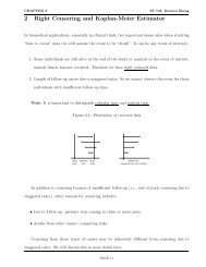
We find it useful to consider a graphical representation <strong>of</strong> the relationship between confidence<br />
intervals and acceptance regions.<br />
PAGE 25
CHAPTER 2 <strong>ST</strong> <strong>520</strong>, A. TSIATIS and D. Zhang<br />
sample space ( X = {0, 1, . . ., n} )<br />
n<br />
k<br />
0<br />
Figure 2.1: Exact confidence intervals<br />
≤ α/2<br />
A(π)<br />
≤ α/2<br />
πL(k) π πU(k)<br />
parameter space (π)<br />
0 1<br />
Another way <strong>of</strong> viewing a (1 − α)-th confidence interval is to find, for each realization X = k,<br />
all the values π ∗ for which the value k would not reject the hypothesis H0 : π = π ∗ . Therefore, a<br />
(1 −α)-th confidence interval is sometimes more appropriately called a (1 −α)-th credible region<br />
(interval).<br />
If X ∼ b(n, π), then when X = k, the (1 − α)-th confidence interval is given by<br />
C(k) = [πL(k), πU(k)],<br />
where πL(k) denotes the lower confidence limit and πU(k) the upper confidence limit, which are<br />
defined as<br />
and<br />
⎛<br />
n� ⎜<br />
PπL(k)(X ≥ k) = ⎝<br />
j=k<br />
n<br />
⎞<br />
⎟<br />
⎠ πL(k)<br />
j<br />
j {1 − πL(k)} n−j = α/2,<br />
⎛<br />
k� ⎜<br />
PπU(k)(X ≤ k) = ⎝<br />
j=0<br />
n<br />
⎞<br />
⎟<br />
⎠ πU(k)<br />
j<br />
j {1 − πU(k)} n−j = α/2.<br />
The values πL(k) and πU(k) need to be evaluated numerically as we will demonstrate shortly.<br />
PAGE 26
CHAPTER 2 <strong>ST</strong> <strong>520</strong>, A. TSIATIS and D. Zhang<br />
Remark: Since X has a discrete distribution, the way we define the (1−α)-th confidence interval<br />
above will yield<br />
Pπ{C(X) ⊃ π} > 1 − α<br />
(strict inequality) for most values <strong>of</strong> 0 ≤ π ≤ 1. Strict equality cannot be achieved because <strong>of</strong><br />
the discreteness <strong>of</strong> the binomial random variable.<br />
Example: In a Phase II clinical trial, 3 <strong>of</strong> 19 patients respond to α-interferon treatment for<br />
multiple sclerosis. In order to find the exact confidence 95% interval for π for X = k, k = 3, and<br />
n = 19, we need to find πL(3) and πU(3) satisfying<br />
PπL(3)(X ≥ 3) = .025; PπU(3)(X ≤ 3) = .025.<br />
Many textbooks have tables for P(X ≤ c), where X ∼ b(n, π) for some n’s and π’s. Alternatively,<br />
P(X ≤ c) can be obtained using statistical s<strong>of</strong>tware such as SAS or R. Either way, we see that<br />
πU(3) ≈ .40. To find πL(3) we note that<br />
PπL(3)(X ≥ 3) = 1 − PπL(3)(X ≤ 2).<br />
Consequently, we must search for πL(3) such that<br />
PπL(3)(X ≤ 2) = .975.<br />
This yields πL(3) ≈ .03. Hence the “exact” 95% confidence interval for π is<br />
[.03, .40].<br />
In contrast, the normal approximation yields a confidence interval <strong>of</strong><br />
� �<br />
3 16 1/2<br />
3<br />
× 19 19<br />
± 1.96 = [−.006, .322].<br />
19 19<br />
PAGE 27
CHAPTER 2 <strong>ST</strong> <strong>520</strong>, A. TSIATIS and D. Zhang<br />
2.2.2 Gehan’s Two-Stage Design<br />
Discarding ineffective treatments early<br />
If it is unlikely that a treatment will achieve some minimal level <strong>of</strong> response or efficacy, we may<br />
want to stop the trial as early as possible. For example, suppose that a 20% response rate is the<br />
lowest response rate that is considered acceptable for a new treatment. If we get no responses in<br />
n patients, with n sufficiently large, then we may feel confident that the treatment is ineffective.<br />
<strong>Statistical</strong>ly, this may be posed as follows: How large must n be so that if there are 0 responses<br />
among n patients we are relatively confident that the response rate is not 20% or better? If<br />
X ∼ b(n, π), and if π ≥ .2, then<br />
Pπ(X = 0) = (1 − π) n ≤ (1 − .2) n = .8 n .<br />
Choose n so that .8 n = .05 or n ln(8) = ln(.05). This leads to n ≈ 14 (rounding up). Thus, with<br />
14 patients, it is unlikely (≤ .05) that no one would respond if the true response rate was greater<br />
than 20%. Thus 0 patients responding among 14 might be used as evidence to stop the phase II<br />
trial and declare the treatment a failure.<br />
This is the logic behind Gehan’s two-stage design. Gehan suggested the following strategy: If<br />
the minimal acceptable response rate is π0, then choose the first stage with n0 patients such that<br />
(1 − π0) n0 = .05; n0 = ln(.05)<br />
ln(1 − π0) ;<br />
if there are 0 responses among the first n0 patients then stop and declare the treatment a failure;<br />
otherwise, continue with additional patients that will ensure a certain degree <strong>of</strong> predetermined<br />
accuracy in the 95% confidence interval.<br />
If, for example, we wanted the 95% confidence interval for the response rate to be within ±15%<br />
when a treatment is considered minimally effective at π0 = 20%, then the sample size necessary<br />
for this degree <strong>of</strong> precision is<br />
�<br />
.2 × .8<br />
1.96<br />
n<br />
�1/2<br />
= .15, or n = 28.<br />
In this example, Gehan’s design would treat 14 patients initially. If none responded, the treatment<br />
would be declared a failure and the study stopped. If there was at least one response, then another<br />
14 patients would be treated and a 95% confidence interval for π would be computed using the<br />
data from all 28 patients.<br />
PAGE 28
CHAPTER 2 <strong>ST</strong> <strong>520</strong>, A. TSIATIS and D. Zhang<br />
2.2.3 Simon’s Two-Stage Design<br />
Another way <strong>of</strong> using two-stage designs was proposed by Richard Simon. Here, the investigators<br />
must decide on values π0, and π1, with π0 < π1 for the probability <strong>of</strong> response so that<br />
• If π ≤ π0, then we want to declare the drug ineffective with high probability, say 1 − α,<br />
where α is taken to be small.<br />
• If π ≥ π1, then we want to consider this drug for further investigation with high probability,<br />
say 1 − β, where β is taken to be small.<br />
The values <strong>of</strong> α and β are generally taken to be between .05 and .20.<br />
The region <strong>of</strong> the parameter space π0 < π < π1 is the indifference region.<br />
Drug is ineffective Indifference region Drug is effective<br />
0 π0<br />
π1<br />
1<br />
π = response rate<br />
A two-stage design would proceed as follows: Integers n1, n, r1, r, with n1 < n, r1 < n1, and<br />
r < n are chosen (to be described later) and<br />
• n1 patients are given treatment in the first stage. If r1 or less respond, then declare the<br />
treatment a failure and stop.<br />
• If more than r1 respond, then add (n − n1) additional patients for a total <strong>of</strong> n patients.<br />
• At the second stage, if the total number that respond among all n patients is greater than<br />
r, then declare the treatment a success; otherwise, declare it a failure.<br />
PAGE 29
CHAPTER 2 <strong>ST</strong> <strong>520</strong>, A. TSIATIS and D. Zhang<br />
<strong>Statistical</strong>ly, this decision rule is the following: Let X1 denote the number <strong>of</strong> responses in the<br />
first stage (among the n1 patients) and X2 the number <strong>of</strong> responses in the second stage (among<br />
the n − n1 patients). X1 and X2 are assumed to be independent binomially distributed random<br />
variables, X1 ∼ b(n1, π) and X2 ∼ b(n2, π), where n2 = n − n1 and π denotes the probability <strong>of</strong><br />
response. Declare the treatment a failure if<br />
otherwise, the treatment is declared a success if<br />
(X1 ≤ r1) or {(X1 > r1) and (X1 + X2 ≤ r)},<br />
{(X1 > r1) and (X1 + X2) > r)}.<br />
Note: If n1 > r and if the number <strong>of</strong> patients responding in the first stage is greater than r,<br />
then there is no need to proceed to the second stage to declare the treatment a success.<br />
According to the constraints <strong>of</strong> the problem we want<br />
or equivalently<br />
P(declaring treatment success|π ≤ π0) ≤ α,<br />
P {(X1 > r1) and (X1 + X2 > r)|π = π0} ≤ α;<br />
(2.1)<br />
� �� �<br />
Note: If the above inequality is true when π = π0, then it is true when π < π0.<br />
Also, we want<br />
or equivalently<br />
P(declaring treatment failure|π ≥ π1) ≤ β,<br />
P {(X1 > r1) and (X1 + X2 > r)|π = π1} ≥ 1 − β. (2.2)<br />
Question: How are probabilities such as P {(X1 > r1) and (X1 + X2 > r)|π} computed?<br />
Since X1 and X2 are independent binomial random variables, then for any integer 0 ≤ m1 ≤ n1<br />
and integer 0 ≤ m2 ≤ n2, the<br />
P(X1 = m1, X2 = m2|π) = P(X1 = m1|π) × P(X2 = m2|π)<br />
⎧⎛<br />
⎪⎨<br />
⎜<br />
= ⎝<br />
⎪⎩<br />
n1<br />
⎞<br />
⎟<br />
⎠π m1<br />
⎫ ⎧⎛<br />
⎪⎬ ⎪⎨<br />
n1−m1 ⎜<br />
(1 − π) ⎝<br />
⎪⎭ ⎪⎩<br />
n2<br />
⎞<br />
⎟<br />
⎠ π m2<br />
⎫<br />
⎪⎬<br />
n2−m2 (1 − π)<br />
⎪⎭ .<br />
m1<br />
PAGE 30<br />
m2
CHAPTER 2 <strong>ST</strong> <strong>520</strong>, A. TSIATIS and D. Zhang<br />
We then have to identify the pairs (m1, m2) where (m1 > r1) and (m1 + m2) > r, find the<br />
probability for each such (m1, m2) pair using the equation above, and then add all the appropriate<br />
probabilities.<br />
We illustrate this in the following figure:<br />
Figure 2.2: Example: n1 = 8, n = 14, X1 > 3, and X1 + X2 > 6<br />
X2<br />
0 1 2 3 4 5 6<br />
0 2 4 6 8<br />
As it turns out there are many combinations <strong>of</strong> (r1, n1, r, n) that satisfy the constraints (2.1) and<br />
(2.2) for specified (π0, π1, α, β). Through a computer search one can find the “optimal design”<br />
among these possibilities, where the optimal design is defined as the combination (r1, n1, r, n),<br />
satisfying the constraints (2.1) and (2.2), which gives the smallest expected sample size when<br />
X1<br />
PAGE 31
CHAPTER 2 <strong>ST</strong> <strong>520</strong>, A. TSIATIS and D. Zhang<br />
π = π0.<br />
The expected sample size for a two stage design is defined as<br />
n1P(stopping at the first stage) + nP(stopping at the second stage).<br />
For our problem, the expected sample size is given by<br />
n1{P(X1 ≤ r1|π = π0) + P(X1 > r|π = π0)} + nP(r1 + 1 ≤ X1 ≤ r|π = π0).<br />
Optimal two-stage designs have been tabulated for a variety <strong>of</strong> (π0, π1, α, β) in the article<br />
Simon, R. (1989). Optimal two-stage designs for Phase II clinical trials. Controlled <strong>Clinical</strong><br />
<strong>Trials</strong>. 10: 1-10.<br />
The tables are given on the next two pages.<br />
PAGE 32
CHAPTER 2 <strong>ST</strong> <strong>520</strong>, A. TSIATIS and D. Zhang<br />
PAGE 33
CHAPTER 2 <strong>ST</strong> <strong>520</strong>, A. TSIATIS and D. Zhang<br />
PAGE 34
CHAPTER 3 <strong>ST</strong> <strong>520</strong>, A. TSIATIS and D. Zhang<br />
3 Phase III <strong>Clinical</strong> <strong>Trials</strong><br />
3.1 Why are clinical trials needed<br />
A clinical trial is the clearest method <strong>of</strong> determining whether an intervention has the postulated<br />
effect. It is very easy for anecdotal information about the benefit <strong>of</strong> a therapy to be accepted<br />
and become standard <strong>of</strong> care. The consequence <strong>of</strong> not conducting appropriate clinical trials can<br />
be serious and costly. As we discussed earlier, because <strong>of</strong> anecdotal information, blood-letting<br />
was common practice for a very long time. Other examples include<br />
• It was believed that high concentrations <strong>of</strong> oxygen was useful for therapy in premature<br />
infants until a clinical trial demonstrated its harm<br />
• Intermittent positive pressure breathing became an established therapy for chronic obstruc-<br />
tive pulmonary disease (COPD). Much later, a clinical trial suggested no major benefit for<br />
this very expensive procedure<br />
• Laetrile (a drug extracted from grapefruit seeds) was rumored to be the wonder drug<br />
for Cancer patients even though there was no scientific evidence that this drug had any<br />
biological activity. People were so convinced that there was a conspiracy by the medical<br />
pr<strong>of</strong>ession to withhold this drug that they would get it illegally from “quacks” or go to<br />
other countries such as Mexico to get treatment. The use <strong>of</strong> this drug became so prevalent<br />
that the National Institutes <strong>of</strong> Health finally conducted a clinical trial where they proved<br />
once and for all that Laetrile had no effect. You no longer hear about this issue any more.<br />
• The Cardiac Antiarhythmia Suppression Trial (CA<strong>ST</strong>) documented that commonly used<br />
antiarhythmia drugs were harmful in patients with myocardial infarction<br />
• More recently, against common belief, it was shown that prolonged use <strong>of</strong> Hormone Re-<br />
placement Therapy for women following menopause may have deleterious effects.<br />
PAGE 35
CHAPTER 3 <strong>ST</strong> <strong>520</strong>, A. TSIATIS and D. Zhang<br />
3.2 Issues to consider before designing a clinical trial<br />
David Sackett gives the following six prerequisites<br />
1. The trial needs to be done<br />
(i) the disease must have either high incidence and/or serious course and poor prognosis<br />
(ii) existing treatment must be unavailable or somehow lacking<br />
(iii) The intervention must have promise <strong>of</strong> efficacy (pre-clinical as well as phase I-II evi-<br />
dence)<br />
2. The trial question posed must be appropriate and unambiguous<br />
3. The trial architecture is valid. Random allocation is one <strong>of</strong> the best ways that treatment<br />
comparisons made in the trial are valid. Other methods such as blinding and placebos<br />
should be considered when appropriate<br />
4. The inclusion/exclusion criteria should strike a balance between efficiency and generaliz-<br />
ibility. Entering patients at high risk who are believed to have the best chance <strong>of</strong> response<br />
will result in an efficient study. This subset may however represent only a small segment<br />
<strong>of</strong> the population <strong>of</strong> individuals with disease that the treatment is intended for and thus<br />
reduce the study’s generalizibility<br />
5. The trial protocol is feasible<br />
(i) The protocol must be attractive to potential investigators<br />
(ii) Appropriate types and numbers <strong>of</strong> patients must be available<br />
6. The trial administration is effective.<br />
Other issues that also need to be considered<br />
• Applicability: Is the intervention likely to be implemented in practice?<br />
• Expected size <strong>of</strong> effect: Is the intervention “strong enough” to have a good chance <strong>of</strong><br />
producing a detectable effect?<br />
PAGE 36
CHAPTER 3 <strong>ST</strong> <strong>520</strong>, A. TSIATIS and D. Zhang<br />
• Obsolescence: Will changes in patient management render the results <strong>of</strong> a trial obsolete<br />
before they are available?<br />
Objectives and Outcome Assessment<br />
• Primary objective: What is the primary question to be answered?<br />
– ideally just one<br />
– important, relevant to care <strong>of</strong> future patients<br />
– capable <strong>of</strong> being answered<br />
• Primary outcome (endpoint)<br />
– ideally just one<br />
– relatively simple to analyze and report<br />
– should be well defined; objective measurement is preferred to a subjective one. For<br />
example, clinical and laboratory measurements are more objective than say clinical<br />
and patient impression<br />
• Secondary Questions<br />
– other outcomes or endpoints <strong>of</strong> interest<br />
– subgroup analyses<br />
– secondary questions should be viewed as exploratory<br />
∗ trial may lack power to address them<br />
∗ multiple comparisons will increase the chance <strong>of</strong> finding “statistically significant”<br />
differences even if there is no effect<br />
– avoid excessive evaluations; as well as problem with multiple comparisons, this may<br />
effect data quality and patient support<br />
PAGE 37
CHAPTER 3 <strong>ST</strong> <strong>520</strong>, A. TSIATIS and D. Zhang<br />
Choice <strong>of</strong> Primary Endpoint<br />
Example: Suppose we are considering a study to compare various treatments for patients with<br />
HIV disease, then what might be the appropriate primary endpoint for such a study? Let us<br />
look at some options and discuss them.<br />
The HIV virus destroys the immune system; thus individuals infected are susceptible to various<br />
opportunistic infections which ultimately leads to death. Many <strong>of</strong> the current treatments are<br />
designed to target the virus either trying to destroy it or, at least, slow down its replication.<br />
Other treatments may target specific opportunistic infections.<br />
Suppose we have a treatment intended to attack the virus directly, Here are some possibilities<br />
for the primary endpoint that we may consider.<br />
1. Increase in CD4 count. Since CD4 count is a direct measure <strong>of</strong> the immune function and<br />
CD4 cells are destroyed by the virus, we might expect that a good treatment will increase<br />
CD4 count.<br />
2. Viral RNA reduction. Measures the amount <strong>of</strong> virus in the body<br />
3. Time to the first opportunistic infection<br />
4. Time to death from any cause<br />
5. Time to death or first opportunistic infection, whichever comes first<br />
Outcomes 1 and 2 may be appropriate as the primary outcome in a phase II trial where we want<br />
to measure the activity <strong>of</strong> the treatment as quickly as possible.<br />
Outcome 4 may be <strong>of</strong> ultimate interest in a phase III trial, but may not be practical for studies<br />
where patients have a long expected survival and new treatments are being introduced all the<br />
time. (Obsolescence)<br />
Outcome 5 may be the most appropriate endpoint in a phase III trial. However, the other<br />
outcomes may be reasonable for secondary analyses.<br />
PAGE 38
CHAPTER 3 <strong>ST</strong> <strong>520</strong>, A. TSIATIS and D. Zhang<br />
3.3 Ethical Issues<br />
A clinical trial involves human subjects. As such, we must be aware <strong>of</strong> ethical issues in the design<br />
and conduct <strong>of</strong> such experiments. Some ethical issues that need to be considered include the<br />
following:<br />
• No alternative which is superior to any trial intervention is available for each subject<br />
• Equipoise–There should be genuine uncertainty about which trial intervention may be<br />
superior for each individual subject before a physician is willing to allow their patients to<br />
participate in such a trial<br />
• Exclude patients for whom risk/benefit ratio is likely to be unfavorable<br />
– pregnant women if possibility <strong>of</strong> harmful effect to the fetus<br />
– too sick to benefit<br />
– if prognosis is good without interventions<br />
Justice Considerations<br />
• Should not exclude a class <strong>of</strong> patients for non medical reasons nor unfairly recruit patients<br />
from poorer or less educated groups<br />
This last issue is a bit tricky as “equal access” may hamper the evaluation <strong>of</strong> interventions. For<br />
example<br />
• Elderly people may die from diseases other than that being studied<br />
• IV drug users are more difficult to follow in AIDS clinical trials<br />
PAGE 39
CHAPTER 3 <strong>ST</strong> <strong>520</strong>, A. TSIATIS and D. Zhang<br />
3.4 The Randomized <strong>Clinical</strong> Trial<br />
The objective <strong>of</strong> a clinical trial is to evaluate the effects <strong>of</strong> an intervention. Evaluation implies<br />
that there must be some comparison either to<br />
• no intervention<br />
• placebo<br />
• best therapy available<br />
Fundamental Principle in Comparing Treatment Groups<br />
Groups must be alike in all important aspects and only differ in the treatment which each group<br />
receives. Otherwise, differences in response between the groups may not be due to the treatments<br />
under study, but can be attributed to the particular characteristics <strong>of</strong> the groups.<br />
How should the control group be chosen<br />
Here are some examples:<br />
• Literature controls<br />
• Historical controls<br />
• Patient as his/her own control (cross-over design)<br />
• Concurrent control (non-randomized)<br />
• Randomized concurrent control<br />
The difficulty in non-randomized clinical trials is that the control group may be different prog-<br />
nostically from the intervention group. Therefore, comparisons between the intervention and<br />
control groups may be biased. That is, differences between the two groups may be due to factors<br />
other than the treatment.<br />
PAGE 40
CHAPTER 3 <strong>ST</strong> <strong>520</strong>, A. TSIATIS and D. Zhang<br />
Attempts to correct the bias that may be induced by these confounding factors either by design<br />
(matching) or by analysis (adjustment through stratified analysis or regression analysis) may not<br />
be satisfactory.<br />
To illustrate the difficulty with non-randomized controls, we present results from 12 different<br />
studies, all using the same treatment <strong>of</strong> 5-FU on patients with advanced carcinoma <strong>of</strong> the large<br />
bowel.<br />
Table 3.1: Results <strong>of</strong> Rapid Injection <strong>of</strong> 5-FU for Treatment <strong>of</strong> Advanced Carcinoma <strong>of</strong> the Large<br />
Bowel<br />
Group # <strong>of</strong> Patients % Objective Response<br />
1. Sharp and Benefiel 13 85<br />
2. Rochlin et al. 47 55<br />
3. Cornell et al. 13 46<br />
4. Field 37 41<br />
5. Weiss and Jackson 37 35<br />
6. Hurley 150 31<br />
7. ECOG 48 27<br />
8. Brennan et al. 183 23<br />
9. Ansfield 141 17<br />
10. Ellison 87 12<br />
11. Knoepp et al. 11 9<br />
12. Olson and Greene 12 8<br />
Suppose there is a new treatment for advanced carcinoma <strong>of</strong> the large bowel that we want to<br />
compare to 5-FU. We decide to conduct a new study where we treat patients only with the new<br />
drug and compare the response rate to the historical controls. At first glance, it looks as if the<br />
response rates in the above table vary tremendously from study to study even though all these<br />
used the same treatment 5-FU. If this is indeed the case, then what comparison can possibly be<br />
made if we want to evaluate the new treatment against 5-FU? It may be possible, however, that<br />
the response rates from study to study are consistent with each other and the differences we are<br />
seeing come from random sampling fluctuations. This is important because if we believe there<br />
is no study to study variation, then we may feel confident in conducting a new study using only<br />
PAGE 41
CHAPTER 3 <strong>ST</strong> <strong>520</strong>, A. TSIATIS and D. Zhang<br />
the new treatment and comparing the response rate to the pooled response rate from the studies<br />
above. How can we assess whether these differences are random sampling fluctuations or real<br />
study to study differences?<br />
Hierarchical Models<br />
To address the question <strong>of</strong> whether the results from the different studies are random samples<br />
from underlying groups with a common response rate or from groups with different underlying<br />
response rates, we introduce the notion <strong>of</strong> a hierarchical model. In a hierarchical model, we<br />
assume that each <strong>of</strong> the N studies that were conducted were from possibly N different study<br />
groups each <strong>of</strong> which have possibly different underlying response rates π1, . . ., πN. In a sense, we<br />
now think <strong>of</strong> the world as being made <strong>of</strong> many different study groups (or a population <strong>of</strong> study<br />
groups), each with its own response rate, and that the studies that were conducted correspond<br />
to choosing a small sample <strong>of</strong> these population study groups. As such, we imagine π1, . . .,πN to<br />
be a random sample <strong>of</strong> study-specific response rates from a larger population <strong>of</strong> study groups.<br />
Since πi, the response rate from the i-th study group, is a random variable, it has a mean and<br />
and a variance which we will denote by µπ and σ 2 π. Since we are imagining a super-population<br />
<strong>of</strong> study groups, each with its own response rate, that we are sampling from, we conceptualize<br />
µπ and σ 2 π to be the average and variance <strong>of</strong> these response rates from this super-population.<br />
Thus π1, . . .,πN will correspond to an iid (independent and identically distributed) sample from<br />
a population with mean µπ and variance σ2 π . I.e.<br />
π1, . . .,πN, are iid with E(πi) = µπ, var(πi) = σ 2 π , i = 1, . . .,N.<br />
This is the first level <strong>of</strong> the hierarchy.<br />
The second level <strong>of</strong> the hierarchy corresponds now to envisioning that the data collected from<br />
the i-th study (ni, Xi), where ni is the number <strong>of</strong> patients treated in the i-th study and Xi is<br />
the number <strong>of</strong> complete responses among the ni treated, is itself a random sample from the i-th<br />
study group whose response rate is πi. That is, conditional on ni and πi, Xi is assumed to follow<br />
a binomial distribution, which we denote as<br />
Xi|ni, πi ∼ b(ni, πi).<br />
This hierarchical model now allows us to distinguish between random sampling fluctuation and<br />
real study to study differences. If all the different study groups were homogeneous, then there<br />
PAGE 42
CHAPTER 3 <strong>ST</strong> <strong>520</strong>, A. TSIATIS and D. Zhang<br />
should be no study to study variation, in which case σ 2 π<br />
<strong>of</strong> study to study differences by estimating the parameter σ 2 π .<br />
= 0. Thus we can evaluate the degree<br />
In order to obtain estimates for σ2 π , we shall use some classical results <strong>of</strong> conditional expectation<br />
and conditional variance. Namely, if X and Y denote random variables for some probability<br />
experiment then the following is true<br />
and<br />
E(X) = E{E(X|Y )}<br />
var(X) = E{var(X|Y )} + var{E(X|Y )}.<br />
Although these results are known to many <strong>of</strong> you in the class; for completeness, I will sketch out<br />
the arguments why the two equalities above are true.<br />
3.5 Review <strong>of</strong> Conditional Expectation and Conditional Variance<br />
For simplicity, I will limit myself to probability experiments with a finite number <strong>of</strong> outcomes.<br />
For random variables that are continuous one needs more complicated measure theory for a<br />
rigorous treatment.<br />
Probability Experiment<br />
Denote the result <strong>of</strong> an experiment by one <strong>of</strong> the outcomes in the sample space Ω = {ω1, . . .,ωk}.<br />
For example, if the experiment is to choose one person at random from a population <strong>of</strong> size N with<br />
a particular disease, then the result <strong>of</strong> the experiment is Ω = {A1, . . .,AN} where the different A’s<br />
uniquely identify the individuals in the population, If the experiment were to sample n individuals<br />
from the population then the outcomes would be all possible n-tuple combinations <strong>of</strong> these N<br />
individuals; for example Ω = {(Ai1, . . ., Ain), for all i1, . . .,in = 1, . . ., N. With replacement<br />
there are k = Nnth combinations; without replacement there are k = N×(N−1)×. . .×(N−n+1)<br />
⎛<br />
⎜<br />
combinations <strong>of</strong> outcomes if order <strong>of</strong> subjects in the sample is important, and k = ⎝ N<br />
⎞<br />
⎟<br />
⎠<br />
n<br />
combinations <strong>of</strong> outcomes if order is not important.<br />
Denote by p(ω) the probability <strong>of</strong> outcome ω occurring, where �<br />
ω∈Ω p(ω) = 1.<br />
PAGE 43
CHAPTER 3 <strong>ST</strong> <strong>520</strong>, A. TSIATIS and D. Zhang<br />
Random variable<br />
A random variable, usually denoted by a capital Roman letter such as X, Y, . . . is a function that<br />
assigns a number to each outcome in the sample space. For example, in the experiment where<br />
we sample one individual from the population<br />
X(ω)= survival time for person ω<br />
Y (ω)= blood pressure for person ω<br />
Z(ω)= height <strong>of</strong> person ω<br />
The probability distribution <strong>of</strong> a random variable X is just a list <strong>of</strong> all different possible<br />
values that X can take together with the corresponding probabilities.<br />
i.e. {(x, P(X = x)), for all possible x}, where P(X = x) = �<br />
ω:X(ω)=x p(ω).<br />
The mean or expectation <strong>of</strong> X is<br />
and the variance <strong>of</strong> X is<br />
E(X) = �<br />
X(ω)p(ω) = �<br />
xP(X = x),<br />
ω∈Ω<br />
var(X) = �<br />
{X(ω) − E(X)} 2 p(ω) = �<br />
{x − E(X)} 2 P(X = x)<br />
ω∈Ω<br />
Conditional Expectation<br />
= E{X − E(X)} 2 = E(X 2 ) − {E(X)} 2 .<br />
Suppose we have two random variables X and Y defined for the same probability experiment, then<br />
we denote the conditional expectation <strong>of</strong> X, conditional on knowing that Y = y, by E(X|Y = y)<br />
and this is computed as<br />
E(X|Y = y) = �<br />
ω:Y (ω)=y<br />
x<br />
x<br />
p(ω)<br />
X(ω)<br />
P(Y = y) .<br />
The conditional expectation <strong>of</strong> X given Y , denoted by E(X|Y ) is itself a random variable which<br />
assigns the value E(X|Y = y) to every outcome ω for which Y (ω) = y. Specifically, we note<br />
that E(X|Y ) is a function <strong>of</strong> Y .<br />
PAGE 44
CHAPTER 3 <strong>ST</strong> <strong>520</strong>, A. TSIATIS and D. Zhang<br />
Since E(X|Y ) is itself a random variable, it also has an expectation given by E{E(X|Y )}. By<br />
the definition <strong>of</strong> expectation this equals<br />
E{E(X|Y )} = �<br />
E(X|Y )(ω)p(ω).<br />
ω∈Ω<br />
By rearranging this sum, first within the partition {ω : Y (ω) = y}, and then across the partitions<br />
for different values <strong>of</strong> y, we get<br />
E{E(X|Y )} = �<br />
��<br />
y<br />
ω:Y (ω)=y X(ω)p(ω)<br />
P(Y = y)<br />
= �<br />
X(ω)p(ω) = E(X).<br />
ω∈Ω<br />
Thus we have proved the very important result that<br />
Conditional Variance<br />
E{E(X|Y )} = E(X).<br />
�<br />
P(Y = y)<br />
There is also a very important relationship involving conditional variance. Just like conditional<br />
expectation. the conditional variance <strong>of</strong> X given Y , denoted as var(X|Y ), is a random variable,<br />
which assigns the value var(X|Y = y) to each outcome ω, where Y (ω) = y, and<br />
var(X|Y = y) = E[{X − E(X|Y = y)} 2 |Y = y] = �<br />
Equivalently,<br />
ω:Y (ω)=y<br />
var(X|Y = y) = E(X 2 |Y = y) − {E(X|Y = y)} 2 .<br />
It turns out that the variance <strong>of</strong> a random variable X equals<br />
This follows because<br />
and<br />
var(X) = E{var(X|Y )} + var{E(X|Y )}.<br />
{X(ω) − E(X|Y = y)} 2 p(ω)<br />
p(Y = y) .<br />
E{var(X|Y )} = E[E(X 2 |Y ) − {E(X|Y )} 2 ] = E(X 2 ) − E[{E(X|Y )} 2 ] (3.1)<br />
var{E(X|Y )} = E[{E(X|Y )} 2 ] − [E{E(X|Y )}] 2 = E[{E(X|Y )} 2 ] − {E(X)} 2<br />
PAGE 45<br />
(3.2)
CHAPTER 3 <strong>ST</strong> <strong>520</strong>, A. TSIATIS and D. Zhang<br />
Adding (3.1) and (3.2) together yields<br />
as desired.<br />
E{var(X|Y )} + var{E(X|Y )} = E(X 2 ) − {E(X)} 2 = var(X),<br />
If we think <strong>of</strong> partitioning the sample space into regions {ω : Y (ω) = y} for different values <strong>of</strong><br />
y, then the formula above can be interpreted in words as<br />
“the variance <strong>of</strong> X is equal to the mean <strong>of</strong> the within partition variances <strong>of</strong> X plus the variance<br />
<strong>of</strong> the within partition means <strong>of</strong> X”. This kind <strong>of</strong> partitioning <strong>of</strong> variances is <strong>of</strong>ten carried out<br />
in ANOVA models.<br />
Return to Hierarchical Models<br />
Recall<br />
and<br />
Xi|ni, πi ∼ b(ni, πi), i = 1, . . ., N<br />
π1, . . .,πN are iid (µπ, σ 2 π ).<br />
Let pi = Xi/ni denote the sample proportion that respond from the i-th study. We know from<br />
properties <strong>of</strong> a binomial distribution that<br />
and<br />
E(pi|πi, ni) = πi<br />
var(pi|πi, ni) = πi(1 − πi)<br />
.<br />
Note: In our conceptualization <strong>of</strong> this problem the probability experiment consists <strong>of</strong><br />
1. Conducting N studies from a population <strong>of</strong> studies<br />
2. For each study i we sample ni individuals at random from the i-th study group and count<br />
the number <strong>of</strong> responses Xi<br />
3. Let us also assume that the sample sizes n1, . . .,nN are random variables from some dis-<br />
tribution.<br />
PAGE 46<br />
ni
CHAPTER 3 <strong>ST</strong> <strong>520</strong>, A. TSIATIS and D. Zhang<br />
4. The results <strong>of</strong> this experiment can be summarized by the iid random vectors<br />
(πi, ni, Xi), i = 1, . . ., N.<br />
In actuality, we don’t get to see the values πi, i = 1, . . .,N. They are implicitly defined, yet very<br />
important in the description <strong>of</strong> the model. Often, the values πi are referred to as random effects.<br />
Thus, the observable data we get to work with are<br />
(ni, Xi), i = 1, . . .,N.<br />
Using the laws <strong>of</strong> iterated conditional expectation and variance just derived, we get the following<br />
results:<br />
E(pi) = E{E(pi|ni, πi)} = E(πi) = µπ, (3.3)<br />
var(pi) = E{var(pi|ni, πi)} + var{E(pi|ni, πi)}<br />
� �<br />
πi(1 − πi)<br />
= E + var(πi)<br />
= E<br />
ni<br />
� �<br />
πi(1 − πi)<br />
ni<br />
+ σ 2 π . (3.4)<br />
Since the random variables pi, i = 1, . . ., N are iid, an unbiased estimator for E(pi) = µπ is<br />
given by the sample mean<br />
¯p = N −1<br />
N�<br />
pi,<br />
i=1<br />
and an unbiased estimator <strong>of</strong> the variance var(pi) is the sample variance<br />
s 2 p =<br />
�Ni=1(pi − ¯p) 2<br />
.<br />
N − 1<br />
One can also show, using properties <strong>of</strong> a binomial distribution, that a conditionally unbiased<br />
estimator for πi(1−πi)<br />
ni<br />
, conditional on ni and πi, is given by pi(1−pi)<br />
; that is<br />
ni−1<br />
E<br />
� pi(1 − pi)<br />
ni − 1 |ni, πi<br />
I will leave this as a homework exercise for you to prove.<br />
�<br />
= πi(1 − πi)<br />
.<br />
ni<br />
Since pi(1−pi)<br />
, i = 1, N are iid random variables with mean<br />
ni−1<br />
� �<br />
E<br />
� pi(1 − pi)<br />
ni − 1<br />
= E<br />
E<br />
PAGE 47<br />
� pi(1 − pi)<br />
ni − 1 |ni, πi<br />
��
CHAPTER 3 <strong>ST</strong> <strong>520</strong>, A. TSIATIS and D. Zhang<br />
� �<br />
πi(1 − πi)<br />
= E ,<br />
this means that we can obtain an unbiased estimator for E � �<br />
πi(1−πi)<br />
by using<br />
N −1<br />
N�<br />
i=1<br />
Summarizing these results, we have shown that<br />
• s 2 p =<br />
� N<br />
(pi−¯p) 2<br />
i=1<br />
N−1<br />
• We have also shown that N −1 � N i=1<br />
ni<br />
pi(1 − pi)<br />
ni − 1 .<br />
is an unbiased estimator for var(pi) which by (3.4) equals<br />
E<br />
� �<br />
πi(1 − πi)<br />
ni<br />
+ σ 2 π<br />
pi(1−pi)<br />
is an unbiased estimator for<br />
ni−1<br />
�<br />
E<br />
� πi(1 − πi)<br />
Consequently, by subtraction, we get that the estimator<br />
ˆσ 2 π =<br />
��Ni=1(pi − ¯p) 2<br />
� �<br />
− N<br />
N − 1<br />
−1<br />
N�<br />
i=1<br />
is an unbiased estimator for σ 2 π.<br />
ni<br />
ni<br />
�<br />
pi(1 − pi)<br />
ni − 1<br />
Going back to the example given in Table 3.1, we obtain the following:<br />
•<br />
•<br />
• Hence<br />
N −1<br />
� Ni=1(pi − ¯p) 2<br />
N − 1<br />
N�<br />
i=1<br />
pi(1 − pi)<br />
ni − 1<br />
= .0496<br />
= .0061<br />
ˆσ 2 π = .0496 − .0061 = .0435<br />
Thus the estimate for study to study standard deviation in the probability <strong>of</strong> response is given<br />
by<br />
ˆσπ = √ .0435 = .21.<br />
This is an enormous variation clearly indicating substantial study to study variation.<br />
PAGE 48
CHAPTER 4 <strong>ST</strong> <strong>520</strong>, A. TSIATIS and D. Zhang<br />
4 Randomization<br />
In a randomized clinical trial, the allocation <strong>of</strong> treatment to patients is carried out using a chance<br />
mechanism so that neither the patient nor the physician knows in advance which treatment will<br />
be assigned. Each patient in the clinical trial has the same opportunity <strong>of</strong> receiving any <strong>of</strong> the<br />
treatments under study.<br />
Advantages <strong>of</strong> Randomization<br />
• Eliminates conscious bias<br />
– physician selection<br />
– patient self selection<br />
• Balances unconscious bias between treatment groups<br />
– supportive care<br />
– patient management<br />
– patient evaluation<br />
– unknown factors affecting outcome<br />
• Groups are alike on average<br />
• Provides a basis for standard methods <strong>of</strong> statistical analysis such as significance tests<br />
4.1 Design-based Inference<br />
On this last point, randomization allows us to carry out design-based inference rather than model-<br />
based inference. That is, the distribution <strong>of</strong> test statistics are induced by the randomization itself<br />
rather than assumptions about a super-population and a probability model. Let me illustrate<br />
through a simple example. Suppose we start by wanting to test the sharp null hypothesis.<br />
Under the sharp null hypothesis, it will be assumed that all the treatments being compared<br />
would yield exactly the same response on all the patients in a study. To test this hypothesis,<br />
patients are randomly allocated to the different treatments and their responses are observed.<br />
PAGE 49
CHAPTER 4 <strong>ST</strong> <strong>520</strong>, A. TSIATIS and D. Zhang<br />
To illustrate, suppose we are comparing two treatments and assign 2 <strong>of</strong> 4 total patients at random<br />
to treatment A and the other 2 to treatment B. Our interest is to see whether one treatment<br />
affects response more than the other. Let’s assume the response is some continuous measurement<br />
which we denote by Y . For example, Y might be the difference in blood pressure one week after<br />
starting treatment.<br />
We will evaluate the two treatments by computing a test statistic corresponding to the difference<br />
in the average response in patients receiving treatment A and the average response in patients<br />
receiving treatment B. If the sharp null hypothesis were true, then we would expect, on average,<br />
the test statistic to be approximately zero; that is the average response for patients receiving<br />
treatment A should be approximately the same as the average response for patients receiving<br />
treatment B. Thus, a value <strong>of</strong> the test statistic sufficiently far from zero could be used as evidence<br />
against the null hypothesis. P-values will be used to measure the strength <strong>of</strong> the evidence. The<br />
p-value is the probability that our test statistic could have taken on a value “more extreme”<br />
than that actually observed, if the experiment were repeated, under the assumption that the null<br />
hypothesis is true. If the p-value is sufficiently small, say < .05 or < .025, then we use this as<br />
evidence to reject the null hypothesis.<br />
Main message: In a randomized experiment, the probability distribution <strong>of</strong> the test statistic<br />
under the null hypothesis is induced by the randomization itself and therefore there is no need<br />
to specify a statistical model about a hypothetical super-population.<br />
We will illustrate this point by our simple example. Let us denote the responses for the two<br />
patients receiving treatment A as y1 and y2 and the responses for the two patients receiving<br />
treatment B as y3 and y4. Thus the value <strong>of</strong> the test statistic based on this data is given by<br />
� � � �<br />
y1 + y2 y3 + y4<br />
T = − .<br />
2 2<br />
How do we decide whether this statistic gives us enough evidence to reject the sharp null hy-<br />
pothesis? More specifically, how do we compute the p-value?<br />
Answer: Under the sharp null hypothesis, the permutational probability distribution <strong>of</strong> our test<br />
static, induced by the randomization, can be evaluated, see Table 4.1.<br />
PAGE 50
CHAPTER 4 <strong>ST</strong> <strong>520</strong>, A. TSIATIS and D. Zhang<br />
Table 4.1: Permutational distribution under sharp null<br />
patient 1 2 3 4<br />
response y1 y2 y3 y4 Test statistic T<br />
possible A A B B � �<br />
y1+y2 − 2<br />
� �<br />
y3+y4 = t1 2<br />
treatment A B A B � �<br />
y1+y3 − 2<br />
� �<br />
y2+y4 = t2 2<br />
assignments A B B A � �<br />
y1+y4 − 2<br />
� �<br />
y2+y3 = t3 2<br />
each B A A B � �<br />
y2+y3 − 2<br />
� �<br />
y1+y4 = t4 2<br />
equally B A B A � �<br />
y2+y4 − 2<br />
� �<br />
y1+y3 = t5 2<br />
likely B B A A � �<br />
y3+y4 − 2<br />
� �<br />
y1+y2 = t6 2<br />
Under the sharp null hypothesis, the test statistic T (i.e. difference in the two means) can take<br />
⎛<br />
⎜<br />
on any <strong>of</strong> the six values t1, . . .,t6, corresponding to the ⎝ 4<br />
⎞<br />
⎟<br />
⎠ = 6 combinations, each with<br />
2<br />
probability 1/6. The value <strong>of</strong> the test statistic actually observed; in this case t1, can be declared<br />
sufficiently large by gauging it according to the probability distribution induced above. That is,<br />
we can compute P(T ≥ t1|sharp null hypothesis), in this case by just counting the number <strong>of</strong> tj<br />
for j = 1, . . .,6 that are greater than or equal to t1 and dividing by six.<br />
Clearly, no one would launch into a comparative trial with only four patients. We used this<br />
example for ease <strong>of</strong> illustration to enumerate the permutational distribution. Nonetheless, for<br />
a larger experiment such an enumeration is possible and the permutational distribution can be<br />
computed exactly or approximated well by computer simulation.<br />
Note: In the above example, we were implicitly testing the null hypothesis against the one-<br />
sided alternative that treatment A was better than treatment B. In this case, larger values <strong>of</strong><br />
T give more evidence against the null hypothesis. If we, instead, were interested in testing the<br />
null hypothesis against a two-sided alternative; that is, that one treatment is different than the<br />
other, then large values <strong>of</strong> the absolute value <strong>of</strong> T (|T |) would be more appropriate as evidence<br />
against the null hypothesis. For a two-sided alternative the p-value would be computed as<br />
P(|T | ≥ t1|sharp null hypothesis). Because <strong>of</strong> the symmetry in the permutational distribution<br />
<strong>of</strong> T about zero, this means that the p-value for a two-sided test would be double the p-value for<br />
the one-sided test (provided the p-value for the one-sided test was less than .5).<br />
PAGE 51
CHAPTER 4 <strong>ST</strong> <strong>520</strong>, A. TSIATIS and D. Zhang<br />
Remark: In evaluating the probability distribution above, we conditioned on the individuals<br />
chosen in the experiment. That is, we took their responses as fixed quantities. Randomness was<br />
induced by the chance assignment <strong>of</strong> treatments to individuals which in turn was used to derive<br />
the probability distribution <strong>of</strong> the test statistic.<br />
Contrast this with the usual statistical model which may be used in such an experiment:<br />
and we are testing the null hypothesis<br />
Y1, Y2 are iid N(µ1, σ 2 )<br />
Y3, Y4 are iid N(µ2, σ 2 )<br />
H0 : µ1 = µ2.<br />
The null hypothesis above would be tested using the t-test, where H0 is rejected when the test<br />
statistic<br />
T =<br />
¯YA − ¯ YB<br />
sp(n −1<br />
A + n −1<br />
B ) 1/2<br />
H0<br />
∼ tnA+nB−2,<br />
is sufficiently large or the p-value computed using a t-distribution with nA + nB − 2 degrees <strong>of</strong><br />
freedom.<br />
Personal Comment: The use <strong>of</strong> the permutational distribution for inference about treatment<br />
efficacy is limiting. Ultimately, we are interested in extending our results from an experimental<br />
sample to some larger population. Therefore, in my opinion, the importance <strong>of</strong> randomization<br />
is not the ability to validly use model free statistical tests as we have just seen, but rather, it<br />
allows us to make causal inference. That is, the results <strong>of</strong> a randomized clinical trial can be<br />
used to infer causation <strong>of</strong> the intervention on the disease outcome.<br />
This is in contrast to non-randomized clinical trials or epidemiological experiments where only<br />
associational inference can be made.<br />
There will be discussion <strong>of</strong> these points later in the semester.<br />
Disadvantages <strong>of</strong> Randomization<br />
• Patients or physician may not care to participate in an experiment involving a chance<br />
mechanism to decide treatment<br />
PAGE 52
CHAPTER 4 <strong>ST</strong> <strong>520</strong>, A. TSIATIS and D. Zhang<br />
• May interfere with physician patient relationship<br />
• Part <strong>of</strong> the resources are expended in the control group; i.e. If we had n patients eligible<br />
for a study and had good and reliable historical control data, then it is more efficient to<br />
put all n patients on the new treatment and compare the response rate to the historical<br />
controls rather than randomizing the patients into two groups, say, n/2 patients on new<br />
treatment and n/2 on control treatment and then comparing the response rates among<br />
these two randomized groups.<br />
How Do We Randomize?<br />
4.2 Fixed Allocation Randomization<br />
This scheme, which is the most widely used, assigns interventions to the participants with a<br />
prespecified probability which is not altered as the study progresses.<br />
Suppose we are considering two treatments. We want to assign patients to one treatment with<br />
probability π and to the other treatment with probability 1 − π. Often π is chosen to be .5.<br />
In some cases, studies have been conducted with unequal allocation probabilities. Let us examine<br />
the consequences <strong>of</strong> the choice <strong>of</strong> randomization probability from a statistical perspective.<br />
Suppose there are n individuals available for study and we allocate nπ ≈ n1 patients to treatment<br />
“1” and n(1 − π) ≈ n2 patients to treatment “2”, with n1 + n2 = n. Say, for example, that the<br />
goal <strong>of</strong> the clinical trial is to estimate the difference in mean response between two treatments;<br />
i.e. we want to estimate<br />
µ2 − µ1,<br />
where µ1 and µ2 denote the population mean response for treatments 1 and 2 respectively.<br />
Remark: As always, some hypothetical population is being envisioned as the population we are<br />
interested in making inference on. If every individual in this population were given treatment 1,<br />
then the mean response (unknown to us) is denoted by µ1; whereas, if every individual in this<br />
hypothetical population were given treatment 2, then the mean response (again unknown to us)<br />
PAGE 53
CHAPTER 4 <strong>ST</strong> <strong>520</strong>, A. TSIATIS and D. Zhang<br />
is denoted by µ2. The n1 and n2 patients that are to be randomized to treatments 1 and 2 are<br />
thought <strong>of</strong> as independent random samples chosen from this hypothetical super-population.<br />
An estimator for the treatment difference is given by<br />
¯Y2 − ¯ Y1,<br />
where ¯ Y1 is the sample average response <strong>of</strong> the n1 patients assigned treatment 1 and ¯ Y2 is the<br />
sample average response <strong>of</strong> the n2 patients assigned treatment 2. Let us also assume that the<br />
population variance <strong>of</strong> response is the same for the two treatments; i.e. σ 2 1 = σ 2 2 = σ 2 . This may<br />
be reasonable if we don’t have any a-priori reason to think these variances are different. The<br />
variance <strong>of</strong> our estimator is given as<br />
var( ¯ Y2 − ¯ Y1) = var( ¯ Y2) + var( ¯ Y1) = σ 2<br />
�<br />
1<br />
n1<br />
+ 1<br />
�<br />
.<br />
n2<br />
Question: Subject to the constraint that n = n1+n2, how do we find the most efficient estimator<br />
for µ2 − µ1? That is, what treatment allocation minimizes the variance <strong>of</strong> our estimator? i.e.<br />
σ 2<br />
�<br />
1<br />
+<br />
n1<br />
1<br />
�<br />
= σ<br />
n2<br />
2<br />
�<br />
1<br />
nπ +<br />
�<br />
1<br />
=<br />
n(1 − π)<br />
σ2<br />
� �<br />
1<br />
.<br />
n π(1 − π)<br />
The answer is the value <strong>of</strong> 0 ≤ π ≤ 1 which maximizes π(1 −π) = π −π 2 . Using simple calculus,<br />
we take the derivative with respect to π and set it equal to zero to find the maximum. Namely,<br />
d(π − π 2 )<br />
dπ<br />
= 1 − 2π = 0; π = .5.<br />
This is guaranteed to be a maximum since the second derivative<br />
d 2 (π − π 2 )<br />
dπ 2<br />
= −2.<br />
Thus, to get the most efficient answer we should randomize with equal probability. However, as<br />
we will now demonstrate, the loss <strong>of</strong> efficiency is not that great when we use unequal allocation.<br />
For example, if we randomize with probability 2/3, then the variance <strong>of</strong> our estimator would be<br />
σ2 � �<br />
1<br />
=<br />
n (2/3)(1/3)<br />
4.5σ2<br />
n<br />
instead <strong>of</strong><br />
σ 2<br />
n<br />
�<br />
1<br />
(1/2)(1/2)<br />
�<br />
PAGE 54<br />
= 4σ2<br />
n ,
CHAPTER 4 <strong>ST</strong> <strong>520</strong>, A. TSIATIS and D. Zhang<br />
with equal allocation.<br />
Another way <strong>of</strong> looking at this relationship is to compute the ratio between the sample sizes<br />
<strong>of</strong> the equal allocation design and the unequal allocation design that yield the same accuracy.<br />
For example, if we randomize with probability 2/3, then to get the same accuracy as the equal<br />
allocation design, we would need<br />
4.5σ 2<br />
n(π=2/3)<br />
= 4σ2<br />
,<br />
n(π=1/2)<br />
where n(π=2/3) corresponds to the sample size for the design with unequal allocation, π = 2/3 in<br />
this case, and n(π=1/2), the sample size for the equal allocation design. It is clear that to get the<br />
same accuracy we need<br />
n(π=2/3)<br />
n(π=1/2)<br />
= 4.5<br />
4<br />
= 1.125.<br />
That is, equal allocation is 12.5% more efficient than a 2:1 allocation scheme; i.e. we need to<br />
treat 12.5% more patients with an unequal allocation (2:1) design to get the same statistical<br />
precision as with an equal allocation (1:1) design.<br />
Some investigators have advocated putting more patients on the new treatment. Some <strong>of</strong> the<br />
reason given include:<br />
• better experience on a drug where there is little information<br />
• efficiency loss is slight<br />
• if new treatment is good (as is hoped) more patients will benefit<br />
• might be more cost efficient<br />
Some disadvantages are:<br />
• might be difficult to justify ethically; It removes equipoise for the participating clinician<br />
• new treatment may be detrimental<br />
PAGE 55
CHAPTER 4 <strong>ST</strong> <strong>520</strong>, A. TSIATIS and D. Zhang<br />
4.2.1 Simple Randomization<br />
For simplicity, let us start by assuming that patients will be assigned to one <strong>of</strong> two treatments<br />
A or B. The methods we will describe will generalize easily to more than two treatments. In<br />
a simple randomized trial, each participant that enters the trial is assigned treatment A or B<br />
with probability π or 1 − π respectively, independent <strong>of</strong> everyone else. Thus, if n patients are<br />
randomized with this scheme, the number <strong>of</strong> patients assigned treatment A is a random quantity<br />
following a binomial distribution ∼ b(n, π).<br />
This scheme is equivalent to flipping a coin (where the probability <strong>of</strong> a head is π) to determine<br />
treatment assignment. Of course, the randomization is implemented with the aid <strong>of</strong> a computer<br />
which generates random numbers uniformly from 0 to 1. Specifically, using the computer, a<br />
sequence <strong>of</strong> random numbers are generated which are uniformly distributed between 0 and 1 and<br />
independent <strong>of</strong> each other. Let us denote these by U1, . . .,Un where Ui are iid U[0, 1]. For the<br />
i-th individual entering the study we would assign treatment as follows:<br />
⎧<br />
⎪⎨ Ui ≤ π then assign treatment A<br />
If<br />
⎪⎩ Ui > π then assign treatment B.<br />
It is easy to see that P(Ui ≤ π) = π, which is the desired randomization probability for treatment<br />
A. As we argued earlier, most <strong>of</strong>ten π is chosen as .5.<br />
Advantages <strong>of</strong> simple randomization<br />
• easy to implement<br />
• virtually impossible for the investigators to guess what the next treatment assignment<br />
will be. If the investigator could break the code, then he/she may be tempted to put<br />
certain patients on preferred treatments thus invalidating the unbiasedness induced by the<br />
randomization<br />
• the properties <strong>of</strong> many statistical inferential procedures (tests and estimators) are established<br />
under the simple randomization assumption (iid)<br />
PAGE 56
CHAPTER 4 <strong>ST</strong> <strong>520</strong>, A. TSIATIS and D. Zhang<br />
Disadvantages<br />
• The major disadvantage is that the number <strong>of</strong> patients assigned to the different treatments<br />
are random. Therefore, the possibility exists <strong>of</strong> severe treatment imbalance.<br />
– leads to less efficiency<br />
– appears awkward and may lead to loss <strong>of</strong> credibility in the results <strong>of</strong> the trial<br />
For example, with n = 20, an imbalance <strong>of</strong> 12:8 or worse can occur by chance with 50% probability<br />
even though π = .5. The problem is not as severe with larger samples. For instance if n = 100,<br />
then a 60:40 split or worse will occur by chance with 5% probability.<br />
4.2.2 Permuted block randomization<br />
One way to address the problem <strong>of</strong> imbalance is to use blocked randomization or, more<br />
precisely, permuted block randomization.<br />
Before continuing, we must keep in mind that patients enter sequentially over time as they become<br />
available and eligible for a study. This is referred to as staggered entry. Also, we must realize that<br />
even with the best intentions to recruit a certain fixed number <strong>of</strong> patients, the actual number<br />
that end up in a clinical trial may deviate from the intended sample size. With these constraints<br />
in mind, the permuted block design is <strong>of</strong>ten used to achieve balance in treatment assignment. In<br />
such a design, as patients enter the study, we define a block consisting <strong>of</strong> a certain number and<br />
proportion <strong>of</strong> treatment assignments. Within each block, the order <strong>of</strong> treatments is randomly<br />
permuted.<br />
For illustration, suppose we have two treatments, A and ⎛B,<br />
and we choose a block size <strong>of</strong> 4,<br />
⎜<br />
with two A’s and two B’s. For each block <strong>of</strong> 4 there are ⎝ 4<br />
⎞<br />
⎟<br />
⎠ or 6 possible combinations <strong>of</strong><br />
2<br />
treatment assignments.<br />
PAGE 57
CHAPTER 4 <strong>ST</strong> <strong>520</strong>, A. TSIATIS and D. Zhang<br />
These are<br />
A A B B<br />
A B A B<br />
A B B A<br />
B A A B<br />
B A B A<br />
B B A A<br />
The randomization scheme, to be described shortly, chooses one <strong>of</strong> these six possibilities with<br />
equal probability (i.e. 1/6) and proceeds as follows. The first four patients entering the trial<br />
are assigned in order to treatments A and B according to the permutation chosen. For the<br />
next block <strong>of</strong> 4, another combination <strong>of</strong> treatment assignments is chosen at random from the six<br />
permutations above and the next four patients are assigned treatments A or B in accordance.<br />
This process continues until the end <strong>of</strong> the study.<br />
It is clear that by using this scheme, the difference in the number <strong>of</strong> patients receiving A versus<br />
B can never exceed 2 regardless when the study ends. Also after every multiple <strong>of</strong> four patients,<br />
the number on treatments A and B are identical.<br />
Choosing random permutations<br />
This can be done by choosing a random number to associate to each <strong>of</strong> the letters “AABB” <strong>of</strong> a<br />
block and then assigning, in order, the letter ranked by the corresponding random number. For<br />
example<br />
Treatment random number rank<br />
A 0.069 1<br />
A 0.734 3<br />
B 0.867 4<br />
B 0.312 2<br />
In the example above the treatment assignment from this block is “ABAB”; that is, A followed by<br />
PAGE 58
CHAPTER 4 <strong>ST</strong> <strong>520</strong>, A. TSIATIS and D. Zhang<br />
B followed by A followed by B. The method just described will guarantee that each combination<br />
is equally likely <strong>of</strong> being chosen.<br />
Potential problem<br />
If the block size b is known in advance, then the clinician may be able to guess what the next<br />
treatment will be. Certainly, the last treatment in a block will be known if the previous treat-<br />
ments have already been assigned. He/she may then be able to bias the results by putting<br />
patients that are at better or worse prognosis on the known treatment. This problem can be<br />
avoided by varying the blocking number at random. For example, the blocking number may be<br />
2,4,6, chosen at random with, say, each with probability 1/3. Varying the block sizes at random<br />
will make it difficult (not impossible) to break the treatment code.<br />
4.2.3 Stratified Randomization<br />
The response <strong>of</strong> individuals <strong>of</strong>ten depends on many different characteristics <strong>of</strong> the patients (other<br />
than treatment) which are <strong>of</strong>ten called prognostic factors. Examples <strong>of</strong> prognostic factors are<br />
age, gender, race, white blood count, Karn<strong>of</strong>sky status. etc. Although randomization balances<br />
prognostic factors “on average” between the different treatments being compared in a study,<br />
imbalances may occur by chance.<br />
If patients with better prognosis end up by luck in one <strong>of</strong> the treatment arms, then one might<br />
question the interpretability <strong>of</strong> the observed treatment differences. One strategy, to minimize<br />
this problem, is to use blocked randomization within strata formed by different combinations<br />
<strong>of</strong> prognostic factors defined a-priori. For example, suppose that age and gender are prognostic<br />
factors that we want to control for in a study. We define strata by breaking down our population<br />
into categories defined by different combinations <strong>of</strong> age and gender.<br />
PAGE 59
CHAPTER 4 <strong>ST</strong> <strong>520</strong>, A. TSIATIS and D. Zhang<br />
Age<br />
Gender 40-49 50-59 60-69<br />
Male<br />
Female<br />
In the illustration above, a total <strong>of</strong> six strata were formed by the 3×2 combinations <strong>of</strong> categories<br />
<strong>of</strong> these two variables.<br />
In a stratified blocked randomization scheme, patients are randomized using block sizes equal<br />
to b (b/2 on each treatment for equal allocation) within each stratum. With this scheme there<br />
could never be a treatment imbalance greater than b/2 within any stratum at any point in the<br />
study.<br />
Advantages <strong>of</strong> Stratified Randomization<br />
• Makes the treatment groups appear similar. This can give more credibility to the results<br />
<strong>of</strong> a study<br />
• Blocked randomization within strata may result in more precise estimates <strong>of</strong> treatment<br />
difference; but one must be careful to conduct the appropriate analysis<br />
Illustration on the effect that blocking within strata has on the precision<br />
<strong>of</strong> estimators<br />
Suppose we have two strata, which will be denoted by the indicator variable S, where<br />
⎧<br />
⎪⎨ 1 = strata 1<br />
S =<br />
⎪⎩ 0 = strata 0.<br />
There are also two treatments denoted by the indicator variable X, where<br />
⎧<br />
⎪⎨ 1 = treatment A<br />
X =<br />
⎪⎩ 0 = treatment B.<br />
Let Y denote the response variable <strong>of</strong> interest. For this illustration, we take Y to be a continuous<br />
random variable; for example, the drop in log viral RNA after three months <strong>of</strong> treatment for HIV<br />
PAGE 60
CHAPTER 4 <strong>ST</strong> <strong>520</strong>, A. TSIATIS and D. Zhang<br />
disease. Consider the following model, where for the i-th individual in our sample, we assume<br />
Yi = µ + αSi + βXi + ǫi. (4.1)<br />
Here α denotes the magnitude <strong>of</strong> effect that strata has on the mean response, β denotes the<br />
magnitude <strong>of</strong> effect that treatment has on the mean response, and the ǫi, i = 1, . . .,n denote<br />
random errors which are taken to be iid random variables with mean zero and variance σ 2 .<br />
Let n individuals be put into a clinical trial to compare treatments A and B and denote by<br />
nA, the number <strong>of</strong> individuals assigned to treatment A; i.e. nA = � n i=1 Xi and nB the number<br />
assigned to treatment B, nB = n − nA.<br />
Let ¯ YA be the average response for the sample <strong>of</strong> individuals assigned to treatment A and ¯ YB<br />
the similar quantity for treatment B:<br />
¯YA = �<br />
Xi=1<br />
¯YB = �<br />
Xi=0<br />
Yi/nA,<br />
Yi/nB.<br />
The objective <strong>of</strong> the study is to estimate treatment effect given, in this case, by the parameter<br />
β. We propose to use the obvious estimator ¯ YA − ¯ YB to estimate β.<br />
Some <strong>of</strong> the patients from both treatments will fall into strata 1 and the others will fall into<br />
strata 0. We represent this in the following table.<br />
Table 4.2: Number <strong>of</strong> observations falling into the different strata by treatment<br />
Because <strong>of</strong> (4.1), we get<br />
¯YA = �<br />
Xi=1<br />
Treatment<br />
strata A B total<br />
0 nA0 nB0 n0<br />
1 nA1 nB1 n1<br />
total nA nB n<br />
Yi/nA<br />
PAGE 61
CHAPTER 4 <strong>ST</strong> <strong>520</strong>, A. TSIATIS and D. Zhang<br />
= �<br />
(µ + αSi + βXi + ǫi)/nA<br />
Xi=1<br />
where ¯ǫA = �<br />
Xi=1 ǫi/nA. Similarly,<br />
where ¯ǫB = �<br />
Xi=0 ǫi/nB. Therefore<br />
Stratified randomization<br />
= (nAµ + α �<br />
Xi=1<br />
Si + β �<br />
Xi=1<br />
= (nAµ + αnA1 + βnA + �<br />
= µ + α nA1<br />
+ β + ¯ǫA,<br />
nA<br />
Xi=1<br />
¯YB = µ + α nB1<br />
+ ¯ǫB,<br />
¯YA − ¯ �<br />
nA1<br />
YB = β + α<br />
nA<br />
nB<br />
Xi + �<br />
Xi=1<br />
ǫi)/nA<br />
ǫi)/nA<br />
− nB1<br />
�<br />
+ (¯ǫA − ¯ǫB). (4.2)<br />
nB<br />
Let us first consider the statistical properties <strong>of</strong> the estimator for treatment difference if we<br />
used permuted block randomization within strata with equal allocation. Roughly speaking, the<br />
number assigned to the two treatments, by strata, would be<br />
nA = nB = n/2<br />
nA1 = nB1 = n1/2<br />
nA0 = nB0 = n0/2.<br />
Remark: The counts above might be <strong>of</strong>f by b/2, where b denotes the block size, but when n is<br />
large this difference is inconsequential.<br />
Substituting these counts into formula (4.2), we get<br />
Note: The coefficient for α cancelled out.<br />
Thus the mean <strong>of</strong> our estimator is given by<br />
¯YA − ¯ YB = β + (¯ǫA − ¯ǫB).<br />
E( ¯ YA − ¯ YB) = E{β + (¯ǫA − ¯ǫB)} = β + E(¯ǫA) − E(¯ǫB) = β,<br />
PAGE 62
CHAPTER 4 <strong>ST</strong> <strong>520</strong>, A. TSIATIS and D. Zhang<br />
which implies that the estimator is unbiased. The variance <strong>of</strong> the estimator is given by<br />
Simple randomization<br />
var( ¯ YA − ¯ YB) = var(¯ǫA) + var(¯ǫB) = σ 2<br />
�<br />
2<br />
n<br />
�<br />
2<br />
+<br />
n<br />
4σ2 . (4.3)<br />
n<br />
With simple randomization the counts nA1 conditional on nA and nB1 conditional on nB follow<br />
a binomial distribution. Specifically,<br />
and<br />
nA1|nA, nB ∼ b(nA, θ) (4.4)<br />
nB1|nA, nB ∼ b(nB, θ), (4.5)<br />
where θ denotes the proportion <strong>of</strong> the population in stratum 1. In addition, conditional on<br />
nA, nB, the binomial variables nA1 and nB1 are independent <strong>of</strong> each other.<br />
The estimator given by (4.2) has expectation equal to<br />
Because <strong>of</strong> (4.4)<br />
Similarly<br />
Hence,<br />
E( ¯ YA − ¯ �<br />
YB) = β + α E<br />
E<br />
� �<br />
nA1<br />
nA<br />
= E<br />
� �<br />
nA1<br />
nA<br />
− E<br />
� ��<br />
nB1<br />
nB<br />
� � ��<br />
nA1<br />
E |nA = E<br />
nA<br />
E<br />
� �<br />
nB1<br />
nB<br />
= θ.<br />
E( ¯ YA − ¯ YB) = β;<br />
+ E(¯ǫA − ¯ǫB). (4.6)<br />
� �<br />
nAθ<br />
= θ.<br />
that is, with simple randomization, the estimator ¯ YA − ¯ YB is an unbiased estimator <strong>of</strong> the<br />
treatment difference β.<br />
In computing the variance, we use the formula for iterated conditional variance; namely<br />
var( ¯ YA − ¯ YB) = E{var( ¯ YA − ¯ YB|nA, nB)} + var{E( ¯ YA − ¯ YB|nA, nB)}.<br />
PAGE 63<br />
nA
CHAPTER 4 <strong>ST</strong> <strong>520</strong>, A. TSIATIS and D. Zhang<br />
As demonstrated above, E( ¯ YA − ¯ YB|nA, nB) = β, thus var{E( ¯ YA − ¯ YB|nA, nB)} = var(β) = 0.<br />
Thus we need to compute E{var( ¯ YA − ¯ YB|nA, nB)}. Note that<br />
Therefore<br />
where nA ∼ b(n, 1/2).<br />
var( ¯ YA − ¯ YB|nA, nB)<br />
� �<br />
nA1<br />
= var β + α −<br />
nA<br />
nB1<br />
�<br />
�<br />
+ (¯ǫA − ¯ǫB)|nA, nB<br />
nB<br />
= α 2<br />
� � � � ��<br />
nA1 nB1<br />
var |nA + var |nB + var(¯ǫA|nA) + var(¯ǫB|nB)<br />
nA nB<br />
= α 2<br />
�<br />
θ(1 − θ)<br />
+ θ(1 − θ)<br />
� � �<br />
2 σ<br />
+<br />
nA<br />
= {σ 2 + α 2 θ(1 − θ)}<br />
nB<br />
� 1<br />
nA<br />
+ 1<br />
nB<br />
nA<br />
�<br />
.<br />
+ σ2<br />
nB<br />
var( ¯ YA − ¯ YB) = E{var( ¯ YA − ¯ YB|nA, nB)}<br />
= {σ 2 + α 2 �<br />
1<br />
θ(1 − θ)}E +<br />
nA<br />
1<br />
�<br />
nB<br />
= {σ 2 + α 2 � �<br />
1 1<br />
θ(1 − θ)}E + ,<br />
nA n − nA<br />
We have already shown that � �<br />
1 1 + nA n−nA<br />
variance <strong>of</strong> the estimator for treatment difference; namely<br />
var( ¯ YA − ¯ YB) = {σ 2 + α 2 θ(1 − θ)}E<br />
≥ 4.<br />
Therefore, with simple randomization the<br />
n<br />
� 1<br />
nA<br />
�<br />
1<br />
+<br />
n − nA<br />
is greater than the variance <strong>of</strong> the estimator for treatment difference with stratified randomiza-<br />
tion; namely<br />
var( ¯ YA − ¯ YB) = 4σ2<br />
n .<br />
Remark: In order to take advantage <strong>of</strong> the greater efficiency <strong>of</strong> the stratified design, one has to<br />
recognize that the variance for ( ¯ YA − ¯ YB) is different when using a stratified design versus simple<br />
randomization. Since many <strong>of</strong> the statistical tests and s<strong>of</strong>tware are based on assumptions that<br />
the data are iid, this point is sometimes missed.<br />
For example, suppose we used a permuted block design within strata but analyzed using a t-test<br />
(the test ordinarily used in conjunction with simple randomization). The t-test is given by<br />
sP<br />
¯YA − ¯ YB<br />
� , 1/2<br />
1<br />
+ nA nB<br />
� 1<br />
PAGE 64
CHAPTER 4 <strong>ST</strong> <strong>520</strong>, A. TSIATIS and D. Zhang<br />
where<br />
s 2 P =<br />
��<br />
Xi=1(Yi − ¯ YA) 2 + �<br />
Xi=0(Yi − ¯ YB) 2<br />
�<br />
.<br />
nA + nB − 2<br />
It turns out that s 2 P is an unbiased estimator for {σ2 + α 2 θ(1 − θ)} as it should be for simple<br />
randomization. However, with stratified randomization, we showed that the variance <strong>of</strong> ( ¯ YA− ¯ YB)<br />
is 4σ2<br />
n .<br />
Therefore the statistic<br />
has variance<br />
sP<br />
¯YA − ¯ YB<br />
� ≈ 1/2<br />
1 + nA nB<br />
� 1<br />
4σ 2 /n<br />
4{σ 2 + α 2 θ(1 − θ)}/n =<br />
¯YA − ¯ YB<br />
{σ 2 + α 2 θ(1 − θ)} 1/2<br />
� 2<br />
n<br />
σ 2<br />
σ 2 + α 2 θ(1 − θ)<br />
� , 1/2<br />
2 + n<br />
Hence the statistic commonly used to test differences in means between two populations<br />
sP<br />
¯YA − ¯ YB<br />
� , 1/2<br />
1<br />
+ nA nB<br />
� 1<br />
does not have a t-distribution if used with a stratified design and α �= 0 (i.e. some strata effect).<br />
In fact, it has a distribution with smaller variance. Thus, if this test were used in conjunction<br />
with a stratified randomized design, then the resulting analysis would be conservative.<br />
The correct analysis would have considered the strata effect in a two-way analysis <strong>of</strong> variance<br />
ANOVA which would then correctly estimate the variance <strong>of</strong> the estimator for treatment effect.<br />
In general, if we use permuted block randomization within strata in the design, we<br />
need to account for this in the analysis.<br />
In contrast, if we used simple randomization and the two-sample t-test, we would be making<br />
correct inference. Even so, we might still want to account for the effect <strong>of</strong> strata post-hoc in the<br />
analysis to reduce the variance and get more efficient estimators for treatment difference. Some<br />
<strong>of</strong> these issues will be discussed later in the course.<br />
Disadvantage <strong>of</strong> blocking within strata<br />
One can inadvertently counteract the balancing effects <strong>of</strong> blocking by having too many strata.<br />
As we consider more prognostic factors to use for balance, we find that the number <strong>of</strong> strata<br />
PAGE 65<br />
≤ 1.
CHAPTER 4 <strong>ST</strong> <strong>520</strong>, A. TSIATIS and D. Zhang<br />
grow exponentially. For example, with 10 prognostic factors, each dichotomized, we would have<br />
2 10 = 1024 strata. In the most extreme case, suppose we have so many strata that there is no<br />
more than one patient per stratum. The result is then equivalent to having simple randomization<br />
and blocking would have no impact at all. Generally, we should use few strata relative to the<br />
size <strong>of</strong> the clinical trial. That is, most blocks should be filled because unfilled blocks permit<br />
imbalances.<br />
4.3 Adaptive Randomization Procedures<br />
This is where the rule for allocation to different treatments may vary according to the results<br />
from prior patients already in the study. Baseline adaptive procedures attempt to balance the<br />
allocation <strong>of</strong> patients to treatment overall and/or by prognostic factors. Some examples are<br />
4.3.1 Efron biased coin design<br />
Choose an integer D, referred to as the discrepancy, and a probability φ less than .5. For example,<br />
we can take D = 3 and φ = .25. The allocation scheme is as follows. Suppose at any point<br />
in time in the study the number <strong>of</strong> patients on treatment A and treatment B are nA and nB<br />
respectively. The next patient to enter the study will be randomized to treatment A or B with<br />
probability πA or 1 − πA, where<br />
πA = .5 if |nA − nB| ≤ D<br />
πA = φ if nA − nB > D<br />
πA = 1 − φ if nB − nA > D<br />
The basic idea is that as soon as the treatments become sufficiently imbalanced favoring one<br />
treatment, then the randomization is chosen to favor the other treatment in an attempt to<br />
balance more quickly while still incorporating randomization so that the physician can never be<br />
certain <strong>of</strong> the next treatment assignment,<br />
A criticism <strong>of</strong> this method is that design-based inference is difficult to implement. Personally, I<br />
don’t think this issue is <strong>of</strong> great concern because model-based inference is generally the accepted<br />
PAGE 66
CHAPTER 4 <strong>ST</strong> <strong>520</strong>, A. TSIATIS and D. Zhang<br />
practice. However, the complexity <strong>of</strong> implementing this method may not be worthwhile.<br />
4.3.2 Urn Model (L.J. Wei)<br />
In this scheme we start with 2m balls in an urn; m labeled A and m labeled B. When the first<br />
patient enters the study you choose a ball at random from the urn and assign that treatment. If<br />
you chose an A ball, you replace that ball in the urn and add an additional B ball. If you chose<br />
a B ball then you replace it and add an additional A ball. Continue in this fashion. Clearly,<br />
the reference to an urn is only for conceptualization, such a scheme would be implemented by a<br />
computer.<br />
Again, as soon as imbalance occurs in favor <strong>of</strong> one treatment, the chances become greater to get<br />
the other treatment in an attempt to balance more quickly. This scheme makes it even more<br />
difficult than the biased coin design for the physician to guess what treatment the next patient<br />
will be assigned to. Again, design-based inference is difficult to implement, but as before, this<br />
may not be <strong>of</strong> concern for most clinical trial statisticians.<br />
Both the biased coin design and the urn model can be implemented within strata.<br />
4.3.3 Minimization Method <strong>of</strong> Pocock and Simon<br />
This is almost a deterministic scheme for allocating treatment with the goal <strong>of</strong> balancing many<br />
prognostic factors (marginally) by treatment. Suppose there are K prognostic factors, indexed<br />
by i = 1, . . ., K and each prognostic factor is broken down into ki levels, then the total number<br />
<strong>of</strong> strata is equal to k1 × . . . × kK. This can be a very large number, in which case, permuted<br />
block randomization within strata may not be very useful in achieving balance. Suppose, instead,<br />
we wanted to achieve some degree <strong>of</strong> balance for the prognostic factors marginally rather than<br />
within each stratum (combination <strong>of</strong> categories from all prognostic factors). Pocock and Simon<br />
suggested using a measure <strong>of</strong> marginal discrepancy where the next patient would be assigned to<br />
whichever treatment that made this measure <strong>of</strong> marginal discrepancy smallest. Only in the case<br />
where the measure <strong>of</strong> marginal discrepancy was the same for both treatments would the next<br />
patient be randomized to one <strong>of</strong> the treatments with equal probability.<br />
PAGE 67
CHAPTER 4 <strong>ST</strong> <strong>520</strong>, A. TSIATIS and D. Zhang<br />
At any point in time in the study, let us denote by nAij the number <strong>of</strong> patients that are on<br />
treatment A for the j-th level <strong>of</strong> prognostic factor i. An analogous definition for nBij.<br />
Note: If nA denotes the total number on treatment A, then<br />
Similarly,<br />
ki �<br />
nA = nAij; for all i = 1, . . ., K.<br />
j=1<br />
ki �<br />
nB = nBij; for all i = 1, . . .,K.<br />
j=1<br />
The measure <strong>of</strong> marginal discrepancy is given by<br />
K� ki �<br />
MD = w0|nA − nB| + wi( |nAij − nBij|).<br />
i=1 j=1<br />
The weights w0, w1, . . .,wK are positive numbers which may differ according to the emphasis you<br />
want to give to the different prognostic factors. Generally w0 = K, w1 = . . . = wK = 1.<br />
The next patient that enters the study is assigned either treatment A or treatment B according<br />
to whichever makes the subsequent measure <strong>of</strong> marginal discrepancy smallest. In case <strong>of</strong> a tie,<br />
the next patient is randomized with probability .5 to either treatment. We illustrate with an<br />
example. For simplicity, consider two prognostic factors, K=2, the first with two levels, k1 = 2<br />
and the second with three levels k2 = 3. Suppose after 50 patients have entered the study, the<br />
marginal configuration <strong>of</strong> counts for treatments A and B, by prognostic factor, looks as follows:<br />
Treatment A Treatment B<br />
PF1 PF1<br />
PF2 1 2 Total PF2 1 2 Total<br />
1 * 13 1 * 12<br />
2 9 2 6<br />
3 4 3 6<br />
Total 16 10 26 Total 14 10 24<br />
If we take the weights to be w0 = 2 and w1 = w2 = 1, then the measure <strong>of</strong> marginal discrepancy<br />
at this point equals<br />
MD = 2|26 − 24| + 1(|16 − 14| + |10 − 10|) + 1(|13 − 12| + |9 − 6| + |4 − 6|) = 12.<br />
PAGE 68
CHAPTER 4 <strong>ST</strong> <strong>520</strong>, A. TSIATIS and D. Zhang<br />
Suppose the next patient entering the study is at the second level <strong>of</strong> PF1 and the first level <strong>of</strong><br />
PF2. Which treatment should that patient be randomized to?<br />
If the patient were randomized to treatment A, then the result would be<br />
and the measure <strong>of</strong> marginal discrepancy<br />
Treatment A Treatment B<br />
PF1 PF1<br />
PF2 1 2 Total PF2 1 2 Total<br />
1 14 1 12<br />
2 9 2 6<br />
3 4 3 6<br />
Total 16 11 27 Total 14 10 24<br />
MD = 2|27 − 24| + 1(|16 − 14| + |11 − 10|) + 1(|14 − 12| + |9 − 6| + |4 − 6|) = 16.<br />
Whereas, if that patient were assigned to treatment B, then<br />
and the measure <strong>of</strong> marginal discrepancy<br />
Treatment A Treatment B<br />
PF1 PF1<br />
PF2 1 2 Total PF2 1 2 Total<br />
1 13 1 13<br />
2 9 2 6<br />
3 4 3 6<br />
Total 16 10 26 Total 14 11 25<br />
MD = 2|26 − 25| + 1(|16 − 14| + |10 − 11|) + 1(|13 − 13| + |9 − 6| + |4 − 6|) = 10.<br />
Therefore, we would assign this patient to treatment B.<br />
Note that design-based inference is not even possible since the allocation is virtually deterministic.<br />
PAGE 69
CHAPTER 4 <strong>ST</strong> <strong>520</strong>, A. TSIATIS and D. Zhang<br />
4.4 Response Adaptive Randomization<br />
In response adaptive schemes, the responses <strong>of</strong> the past participants in the study are used to<br />
determine the treatment allocation for the next patient. Some examples are<br />
Play-the-Winner Rule (Zelen)<br />
• First patient is randomized to either treatment A or B with equal probability<br />
• Next patient is assigned the same treatment as the previous one if the previous patient’s<br />
response was a success; whereas, if the previous patient’s response is a failure, then the<br />
patient receives the other treatment. The process calls for staying with the winner until a<br />
failure occurs and then switching.<br />
For example,<br />
Urn Model (L.J. Wei)<br />
Patient ordering<br />
Treatment 1 2 3 4 5 6 7 8<br />
A S F S S F<br />
B S S F<br />
The first patient is assigned to either treatment by equal probability. Then every time there is<br />
a success on treatment A add r A balls into the urn, when there is a failure on treatment A add<br />
r B balls. Similarly for treatment B. The next patient is assigned to whichever ball is drawn at<br />
random from this urn.<br />
Response adaptive allocation schemes have the intended purpose <strong>of</strong> maximizing the number <strong>of</strong><br />
patients in the trial that receive the superior treatment.<br />
Difficulties with response adaptive allocation schemes<br />
• Information on response may not be available immediately.<br />
PAGE 70
CHAPTER 4 <strong>ST</strong> <strong>520</strong>, A. TSIATIS and D. Zhang<br />
• Such strategies may take a greater number <strong>of</strong> patients to get the desired answer. Even<br />
though more patients on the trial may be getting the better treatment, by taking a longer<br />
time, this better treatment is deprived from the population at large who may benefit.<br />
• May interfere with the ethical principle <strong>of</strong> equipoise.<br />
• Results may not be easily interpretable from such a design.<br />
ECMO trial<br />
To illustrate the last point, we consider the results <strong>of</strong> the ECMO trial which used a play-the-<br />
winner rule.<br />
Extracorporeal membrane oxygenator was a promising treatment for a neonatal population suf-<br />
fering from respiratory insufficiency. This device oxygenates the blood to compensate for the<br />
lung’s inability or inefficiency in achieving this task. Because the mortality rate was very high<br />
for this population and because <strong>of</strong> the very promising results <strong>of</strong> ECMO it was decided to use a<br />
play-the-winner rule.<br />
The first child was randomized to the control group and died. The next 10 children were assigned<br />
ECMO and all survived at which point the trial was stopped and ECMO declared a success.<br />
It turned out that after further investigation, the first child was the sickest <strong>of</strong> all the children<br />
studied. Controversy ensued and the study had to be repeated using a more traditional design.<br />
Footnote on page 73 <strong>of</strong> the textbook FFD gives further references.<br />
4.5 Mechanics <strong>of</strong> Randomization<br />
The following formal sequence <strong>of</strong> events should take place before a patient is randomized into a<br />
phase III clinical trial.<br />
• Patient requires treatment<br />
• Patient is eligible for the trial. Inclusion and exclusion criteria should be checked immedi-<br />
ately. For a large multi-center trial, this may be done at a central registration <strong>of</strong>fice<br />
PAGE 71
CHAPTER 4 <strong>ST</strong> <strong>520</strong>, A. TSIATIS and D. Zhang<br />
• Clinician is willing to accept randomization<br />
• Patient consent is obtained. In the US this is a legal requirement<br />
• Patient formally entered into the trial<br />
After a patient and his/her physician agree to participate in the trial then<br />
• Each patient must be formally identified. This can be done by collecting some minimal<br />
information; i.e. name, date <strong>of</strong> birth, hospital number. This information should be kept<br />
on a log (perhaps at a central <strong>of</strong>fice) and given a trial ID number for future identification.<br />
This helps keep track <strong>of</strong> the patient and it helps guard against investigators not giving the<br />
allocated treatment.<br />
• The treatment assignment is obtained from a randomization list. Most <strong>of</strong>ten prepared in<br />
advance<br />
(a) The randomization list could be transferred to a sequence <strong>of</strong> sealed envelopes each<br />
containing the name <strong>of</strong> the next treatment on the card. The clinician opens the<br />
envelope when a patient has been formerly registered onto the trial<br />
(b) If the trial is double-blind then the pharmacist preparing the drugs needs to be in-<br />
volved. They prepare the sequence <strong>of</strong> drug packages according to the randomization<br />
list.<br />
(c) For a multi-center trial, randomization is carried out by the central <strong>of</strong>fice by phone or<br />
by computer.<br />
(d) For a double-blind multi-center trial, the randomization may need to be decentralized<br />
Documentation<br />
to each center according to (b). However, central registration is recommended.<br />
• A confirmation form needs to be filled out after treatment assignment which contains name,<br />
trial number and assigned treatment. If randomization is centralized then this confirmation<br />
form gets sent from the central <strong>of</strong>fice to the physician. If it is decentralized then it goes<br />
from physician to central <strong>of</strong>fice.<br />
PAGE 72
CHAPTER 4 <strong>ST</strong> <strong>520</strong>, A. TSIATIS and D. Zhang<br />
• An on-study form is then filled out containing all relevant information prior to treatment<br />
such as previous therapies, personal characteristics (age, race, gender, etc.), details about<br />
clinical conditions and certain laboratory tests (e.g. lung function for respiratory illness)<br />
All <strong>of</strong> these checks and balances must take place quickly but accurately prior to the patient<br />
commencing therapy.<br />
PAGE 73
CHAPTER 5 <strong>ST</strong> <strong>520</strong>, A. TSIATIS and D. Zhang<br />
5 Some Additional Issues in Phase III <strong>Clinical</strong> <strong>Trials</strong><br />
5.1 Blinding and Placebos<br />
Even in a randomized trial the comparison <strong>of</strong> treatments may be distorted if the patients and<br />
those responsible for administering the treatment and evaluation know which treatment is being<br />
used. These problems can be avoided in some cases by making the trial double blind, whereby,<br />
neither patient, physician nor evaluator are aware which treatment the patient is receiving.<br />
• The patient— If the patient knows he/she is receiving a new treatment then this may result<br />
in psychological benefit. The degree <strong>of</strong> psychological effect depends on the type <strong>of</strong> disease<br />
and the nature <strong>of</strong> treatments. One should not underestimate the importance <strong>of</strong> psychology<br />
for patients with disease. Whether it is asthma, cancer, heart disease, etc, the manner in<br />
which patients are informed <strong>of</strong> therapy has a pr<strong>of</strong>ound effect on subsequent performance.<br />
• The treatment team—(anyone who participates in the treatment or management <strong>of</strong> the<br />
patient). Patients known to be receiving a new therapy may be treated differently than<br />
those on standard treatment. Such difference in ancillary care may affect the response.<br />
• The evaluator— It is especially important that the individual or individuals evaluating<br />
response be objective. A physician who has pre-conceived ideas how a new treatment<br />
might work may introduce bias in his/her evaluation <strong>of</strong> the patient response if they know<br />
the treatment that the patient received.<br />
The biases above may be avoided with proper blinding. However, blinding treatments takes<br />
a great deal <strong>of</strong> care and planning. If the treatment is in the form <strong>of</strong> pills, then the pills for<br />
the different treatments should be indistinguishable; i.e the same size, color, taste, texture.<br />
If no treatment is to be used as the control group then we may consider using a placebo for<br />
patients randomized to the control group. A placebo is a pill or other form <strong>of</strong> treatment which is<br />
indistinguishable from the active treatment but contains no active substance. (sugar pill, saline,<br />
etc.) If you are comparing two active treatments each, say, with pills that cannot be made to<br />
be similar, then we may have to give each patient two pills; one active pill for one treatment<br />
PAGE 74
CHAPTER 5 <strong>ST</strong> <strong>520</strong>, A. TSIATIS and D. Zhang<br />
and a placebo pill for the other treatment. (This can become overwhelming if we are comparing<br />
different combinations <strong>of</strong> drugs).<br />
It has been well documented that there is a placebo effect. That is, there have been randomized<br />
studies conducted that gave some patients placebo and the other patients nothing with the<br />
placebo group responding significantly better. Consequently, in a randomized clinical trial which<br />
compares a new drug to a placebo control, we are actually testing whether the active drug has<br />
effect equal to or greater than a placebo effect.<br />
One must realize that although the principles <strong>of</strong> blinding are good, they are not feasible in some<br />
trials. For example, if we are comparing surgery versus chemotherapy in a cancer clinical trial,<br />
there is no way to blind these treatments. In such cases we must be as careful as possible to<br />
choose endpoints that are as objective as possible. For example, time to death from any cause.<br />
5.2 Ethics<br />
<strong>Clinical</strong> trials are ethical in the setting <strong>of</strong> uncertainty.<br />
PAGE 75
CHAPTER 5 <strong>ST</strong> <strong>520</strong>, A. TSIATIS and D. Zhang<br />
The Hippocratic Oath<br />
I swear by Apollo the physician, by Aesculapius, Hygeia and Panacea, and I take to witness all<br />
the gods, all the goddesses, to keep according to my ability and my judgment the following Oath:<br />
To consider dear to me as my parents him who taught me this art; to live in common with him<br />
and if necessary to share my goods with him; to look upon his children as my own brothers, to<br />
teach them this art if they so desire without fee or written promise; to impart to my sons and the<br />
sons <strong>of</strong> the master who taught me and the disciples who have enrolled themselves and have agreed<br />
to the rules <strong>of</strong> the pr<strong>of</strong>ession, but to these alone, the precepts and the instruction. I will prescribe<br />
regimen for the good <strong>of</strong> my patients according to my ability and my judgment and never do harm<br />
to anyone. To please no one will I prescribe a deadly drug, nor give advice which may cause his<br />
death. Nor will I give a woman a pessary to procure abortion. But I will preserve the purity <strong>of</strong><br />
my life and my art. I will not cut for stone, even for patients in whom disease is manifest; I<br />
will leave this operation to be performed by practitioners (specialists in this art). In every house<br />
where I come I will enter only for the good <strong>of</strong> my patients, keeping myself far from all intentional<br />
ill-doing and all seduction, and especially from the pleasures <strong>of</strong> love with women or men, be they<br />
free or slaves. All that may come to my knowledge in the exercise <strong>of</strong> my pr<strong>of</strong>ession or outside <strong>of</strong><br />
my pr<strong>of</strong>ession or in daily commerce with men, which ought not to be spread abroad, I will keep<br />
secret and I will never reveal. If I keep this oath faithfully, may I enjoy life and practice my art,<br />
respected by all men and in all times; but if I swerve from it or violate it, may the reverse be my<br />
lot.<br />
PAGE 76
CHAPTER 5 <strong>ST</strong> <strong>520</strong>, A. TSIATIS and D. Zhang<br />
Even today physicians may take the Hippocratic oath although it is not repeated in full. Clearly<br />
many <strong>of</strong> the issues, such as abortion, surgery for kidney stones, use <strong>of</strong> deadly drugs, no longer<br />
apply. Nor does the pledge for “free instruction” still apply.<br />
Ethical considerations have been addressed by the Nuremberg Code and Helsinki Declaration<br />
(see the class website for more details)<br />
In the United States, the Congress established the National Commission for the Protection <strong>of</strong><br />
Human Subjects <strong>of</strong> Biomedical and Behavioral Research as part <strong>of</strong> the National Research Act.<br />
This act required the establishment <strong>of</strong> an Institutional Review Board (IRB) for all research<br />
funded in whole or in part by the federal government. These were later modified to require IRB<br />
approval for all drugs or products regulated by the Food and Drug Administration (FDA).<br />
IRB’s must have at least five members with expertise relevant to safeguarding the rights and<br />
welfare <strong>of</strong> patients participating in biomedical research. At least one should be a scientist, and at<br />
least one must not be affiliated with the institution. The IRB should be made up <strong>of</strong> individuals<br />
with diverse racial, gender and cultural backgrounds. The scope <strong>of</strong> the IRB includes, but is not<br />
limited to consent procedures and research design.<br />
IRB’s approve human research studies that meet specific prerequisites.<br />
(1) The risks to the study participants are minimized<br />
(2) The risks are reasonable in relation to the anticipated benefit<br />
(3) The selection <strong>of</strong> study patients is equitable<br />
(4) Informed consent is obtained and appropriately documented for each participant<br />
(5) There are adequate provisions for monitoring data collected to ensure the safety <strong>of</strong> the<br />
study participants<br />
(6) The privacy <strong>of</strong> the participants and confidentiality <strong>of</strong> the data are protected<br />
5.3 The Protocol Document<br />
Definition: The protocol is a scientific planning document for a medical study on human sub-<br />
PAGE 77
CHAPTER 5 <strong>ST</strong> <strong>520</strong>, A. TSIATIS and D. Zhang<br />
jects. It contains the study background, experimental design, patient population, treatment and<br />
evaluation details, and data collection procedures.<br />
Purposes<br />
(1) To assist investigators in thinking through the research<br />
(2) To ensure that both patient and study management are considered at the planning stage<br />
(3) To provide a sounding board for external comments<br />
(4) To orient the staff for preparation <strong>of</strong> forms and processing procedures<br />
(5) To provide a document which can be used by other investigators who wish to confirm<br />
(replicate) the results<br />
I will hand out two protocols in class. One is from the Womens Health Initiative (WHI) and one<br />
from the Cancer and Leukemia Group B (CALGB) study 8541.<br />
In the WHI study, the clinical trial will evaluate the benefits and risks <strong>of</strong> Hormone Replacement<br />
Therapy (HRT), Dietary Modification, DM, and supplementation with calcium/vitamin D (CaD)<br />
on the overall health <strong>of</strong> postmenopausal women. Health will be assessed on the basis <strong>of</strong> quality<br />
<strong>of</strong> life measurements, cause-specific morbidity and mortality, and total mortality.<br />
CALGB 8541 is a study <strong>of</strong> different regimen <strong>of</strong> adjuvant CAF (combination <strong>of</strong> Cyclophosphamide,<br />
Adriamycin and 5 Fluorouracil (5-FU)) as treatment for women with pathological stage II, node<br />
positive breast cancer. Specifically, intensive CAF for four cycles versus low dose CAF for four<br />
cycles versus standard dose CAF for six cycles will be compared in a three arm randomized<br />
clinical trial.<br />
Protocols generally have the following elements:<br />
1. Schema. Depicts the essentials <strong>of</strong> a study design.<br />
WHI: page 18<br />
CALGB 8541: page 1<br />
PAGE 78
CHAPTER 5 <strong>ST</strong> <strong>520</strong>, A. TSIATIS and D. Zhang<br />
2. Objectives The objectives should be few in number and should be based on specific<br />
quantifiable endpoints<br />
WHI: pages 14-15 and pages 22-24<br />
CALGB 8541: page 3<br />
3. Project background This section should give the referenced medical/historical back-<br />
ground for therapy <strong>of</strong> these patients.<br />
WHI: pages 2-13<br />
CALGB 8541: pages 1-3<br />
This generally includes<br />
– standard therapy<br />
– predecessor studies (phase I and II if appropriate)<br />
– previous or concurrent studies <strong>of</strong> a similar nature<br />
– moral justification <strong>of</strong> the study<br />
4. Patient Selection A clear definition <strong>of</strong> the patient population to be studied. This should<br />
include clear, unambiguous inclusion and exclusion criteria that are verifiable at the time<br />
<strong>of</strong> patient entry. Each item listed should be verified on the study forms.<br />
WHI: pages 24-28<br />
CALGB 8541: pages 4-5<br />
5. Randomization/Registration Procedures This section spells out the mechanics <strong>of</strong><br />
entering a patient into the study<br />
WHI: pages 29-38<br />
CALGB 8541: pages 5-7<br />
6. Treatment Administration and Patient Management How the treatment is to be<br />
administered needs to be specified in detail. All practical eventualities should be taken<br />
into account, at least, as much as possible. Protocols should not be written with only the<br />
study participants in mind. Others may want to replicate this therapy such as community<br />
hospitals that were not able to participate in the original study.<br />
WHI: pages 18-22 and 44-49<br />
CALGB 8541: pages 7-20<br />
PAGE 79
CHAPTER 5 <strong>ST</strong> <strong>520</strong>, A. TSIATIS and D. Zhang<br />
7. Study parameters This section gives the schedule <strong>of</strong> the required and optional investi-<br />
gations/tests.<br />
WHI: pages 38-39<br />
CALGB 8541: page 20<br />
8. <strong>Statistical</strong> Considerations<br />
WHI: pages 52-55 and an extensive appendix (not provided)<br />
CALGB 8541: pages 22-23<br />
– Study outline, stratification and randomization<br />
– Sample size criteria: Motivation for the sample size and duration <strong>of</strong> the trial needs to<br />
be given. This can be based on type I and type II error considerations in a hypothesis<br />
testing framework or perhaps based on the desired accuracy <strong>of</strong> a confidence interval.<br />
– Accrual estimates<br />
– Power calculations<br />
– Brief description <strong>of</strong> the data analysis that will be used<br />
– Interim monitoring plans<br />
9. Informed Consent The consent form needs to be included.<br />
For both WHI and CALGB 8541 these are in an appendix (not included)<br />
The informed consent should include<br />
– an explanation <strong>of</strong> the procedures to be followed and their purposes<br />
– a description <strong>of</strong> the benefits that might reasonably be expected<br />
– a description <strong>of</strong> the discomforts and risks that could reasonably be expected<br />
– a disclosure <strong>of</strong> any appropriate alternative procedures that might be advantageous<br />
– a statement that the subject is at liberty to abstain from participation in the study<br />
and is free to withdraw at any time<br />
10. Study Management Policy This section includes how the study will be organized and<br />
managed, when the data will be summarized and the details <strong>of</strong> manuscript development<br />
and publication<br />
WHI: pages 58-61<br />
CALGB 8541: Was not included<br />
PAGE 80
CHAPTER 6 <strong>ST</strong> <strong>520</strong>, A. TSIATIS and D. Zhang<br />
6 Sample Size Calculations<br />
One <strong>of</strong> the major responsibilities <strong>of</strong> a clinical trial statistician is to aid the investigators in<br />
determining the sample size required to conduct a study. The most common procedure for<br />
determining the sample size involves computing the minimum sample size necessary in order that<br />
important treatment differences be determined with sufficient accuracy. We will focus primarily<br />
on hypothesis testing.<br />
6.1 Hypothesis Testing<br />
In a hypothesis testing framework, the question is generally posed as a decision problem regarding<br />
a parameter in a statistical model:<br />
Suppose a population parameter corresponding to a measure <strong>of</strong> treatment difference using the<br />
primary endpoint is defined for the study. This parameter will be denoted by ∆. For example,<br />
if we are considering the mean response <strong>of</strong> some continuous variable between two treatments, we<br />
can denote by µ1, the population mean response for treatment 1 and µ2, the mean response on<br />
treatment 2. We then denote by<br />
∆ = µ1 − µ2<br />
the measure <strong>of</strong> treatment difference. A clinical trial will be conducted in order to make inference<br />
on this population parameter. If we take a hypothesis testing point <strong>of</strong> view, then we would<br />
consider the following decision problem: Suppose treatment 2 is currently the standard <strong>of</strong> care<br />
and treatment 1 is a new treatment that has shown promise in preliminary testing. What we<br />
want to decide is whether we should recommend the new treatment or stay with the standard<br />
treatment. As a starting point we might say that if, in truth, ∆ ≤ 0 then we would want to<br />
stay with the standard treatment; whereas, if, in truth, ∆ > 0, then we would recommend that<br />
future patients go on the new treatment. We refer to ∆ ≤ 0 as the null hypothesis “H0” and<br />
∆ > 0 as the alternative hypothesis “HA”. The above is an example <strong>of</strong> a one-sided hypothesis<br />
test. In some cases, we may be interested in a two-sided hypothesis test where we test the null<br />
hypothesis H0 : ∆ = 0 versus the alternative HA : ∆ �= 0.<br />
In order to make a decision on whether to choose the null hypothesis or the alternative hypothesis,<br />
PAGE 81
CHAPTER 6 <strong>ST</strong> <strong>520</strong>, A. TSIATIS and D. Zhang<br />
we conduct a clinical trial and collect data from a sample <strong>of</strong> individuals. The data from n<br />
individuals in our sample will be denoted generically as (z1, . . .,zn) and represent realizations <strong>of</strong><br />
random vectors (Z1, . . .,Zn). The Zi may represent a vector <strong>of</strong> random variables for individual<br />
i; e.g. response, treatment assignment, other covariate information.<br />
As statisticians, we posit a probability model that describes the distribution <strong>of</strong> (Z1, . . .,Zn) in<br />
terms <strong>of</strong> population parameters which includes ∆ (treatment difference) as well as other param-<br />
eters necessary to describe the probability distribution. These other parameters are referred to<br />
as nuisance parameters. We will denote the nuisance parameters by the vector θ. As a simple<br />
example, let the data for the i-th individual in our sample be denoted by Zi = (Yi, Ai), where<br />
Yi denotes the response (taken to be some continuous measurement) and Ai denotes treatment<br />
assignment, where Ai can take on the value <strong>of</strong> 1 or 2 depending on the treatment that patient i<br />
was assigned. We assume the following statistical model: let<br />
and<br />
(Yi|Ai = 2) ∼ N(µ2, σ 2 )<br />
(Yi|Ai = 1) ∼ N(µ2 + ∆, σ 2 ),<br />
i.e. since ∆ = µ1 − µ2, then µ1 = µ2 + ∆. The parameter ∆ is the test parameter (treatment<br />
difference <strong>of</strong> primary interest) and θ = (µ2, σ 2 ) are the nuisance parameters.<br />
Suppose we are interested in testing H0 : ∆ ≤ 0 versus HA : ∆ > 0. The way we generally<br />
proceed is to combine the data into a summary test statistic that is used to discriminate between<br />
the null and alternative hypotheses based on the magnitude <strong>of</strong> its value. We refer to this test<br />
statistic by<br />
Tn(Z1, . . ., Zn).<br />
Note: We write Tn(Z1, . . .,Zn) to emphasize the fact that this statistic is a function <strong>of</strong> all the<br />
data Z1, . . .,Zn and hence is itself a random variable. However, for simplicity, we will most <strong>of</strong>ten<br />
refer to this test statistic as Tn or possibly even T.<br />
The statistic Tn should be constructed in such a way that<br />
(a) Larger values <strong>of</strong> Tn are evidence against the null hypothesis in favor <strong>of</strong> the alternative<br />
PAGE 82
CHAPTER 6 <strong>ST</strong> <strong>520</strong>, A. TSIATIS and D. Zhang<br />
(b) The probability distribution <strong>of</strong> Tn can be evaluated (or at least approximated) at the<br />
border between the null and alternative hypotheses; i.e. at ∆ = 0.<br />
After we conduct the clinical trial and obtain the data, i.e. the realization (z1, . . .,zn) <strong>of</strong><br />
(Z1, . . .,Zn), we can compute tn = Tn(z1, . . .,zn) and then gauge this observed value against<br />
the distribution <strong>of</strong> possible values that Tn can take under ∆ = 0 to assess the strength <strong>of</strong><br />
evidence for or against the null hypothesis. This is done by computing the p-value<br />
P∆=0(Tn ≥ tn).<br />
If the p-value is small, say, less than .05 or .025, then we use this as evidence against the null<br />
hypothesis.<br />
Note:<br />
1. Most test statistics used in practice have the property that P∆(Tn ≥ x) increases as ∆<br />
increases, for all x. In particular, this would mean that if the p-value P∆=0(Tn ≥ tn) were<br />
less than α at ∆ = 0, then the probability P∆(Tn ≥ tn) would also be less than α for all ∆<br />
corresponding to the null hypothesis H0 : ∆ ≤ 0.<br />
2. Also, most test statistics are computed in such a way that the distribution <strong>of</strong> the test<br />
statistic, when ∆ = 0, is approximately a standard normal; i.e.<br />
Tn<br />
(∆=0)<br />
∼ N(0, 1),<br />
regardless <strong>of</strong> the values <strong>of</strong> the nuisance parameters θ.<br />
For the problem where we were comparing the mean response between two treatments, where<br />
response was assumed normally distributed with equal variance by treatment, but possibly dif-<br />
ference means, we would use the two-sample t-test; namely,<br />
Tn =<br />
sY<br />
¯Y1 − ¯ Y2<br />
� , 1/2<br />
1<br />
+ n1 n2<br />
� 1<br />
where ¯ Y1 denotes the sample average response among the n1 individuals assigned to treatment<br />
1, ¯ Y2 denotes the sample average response among the n2 individuals assigned to treatment 2,<br />
PAGE 83
CHAPTER 6 <strong>ST</strong> <strong>520</strong>, A. TSIATIS and D. Zhang<br />
n = n1 + n2 and the sample variance is<br />
s 2 Y =<br />
��n1 j=1(Y1j − ¯ Y1) 2 + �n2 j=1(Y2j − ¯ Y2) 2<br />
�<br />
(n1 + n2 − 2)<br />
Under ∆ = 0, the statistic Tn follows a central t distribution with n1 +n2 −2 degrees <strong>of</strong> freedom.<br />
If n is large (as it generally is for phase III clinical trials), this distribution is well approximated<br />
by the standard normal distribution.<br />
If the decision to reject the null hypothesis is based on the p-value being less that α (.05 or .025<br />
generally), then this is equivalent to rejecting H0 whenever<br />
Tn ≥ Zα,<br />
where Zα denotes the 1 − α-th quantile <strong>of</strong> a standard normal distribution; e.g. Z.05 = 1.64 and<br />
Z.025 = 1.96. We say that such a test has level α.<br />
Remark on two-sided tests: If we are testing the null hypothesis H0 : ∆ = 0 versus the<br />
alternative hypothesis HA : ∆ �= 0 then we would reject H0 when the absolute value <strong>of</strong> the test<br />
statistic |Tn| is sufficiently large. The p-value for a two-sided test is defined as P∆=0(|Tn| ≥ tn),<br />
which equals P∆=0(Tn ≥ tn)+P∆=0(Tn ≤ −tn). If the test statistic Tn is distributed as a standard<br />
normal when ∆ = 0, then a level α two-sided test would reject the null hypothesis whenever the<br />
p-value is less than α; or equivalently<br />
|Tn| ≥ Zα/2.<br />
The rejection region <strong>of</strong> a test is defined as the set <strong>of</strong> data points in the sample space that<br />
would lead to rejecting the null hypothesis. For one sided level α tests, the rejection region is<br />
{(z1, . . .,zn) : Tn(z1, . . .,zn) ≥ Zα},<br />
and for two-sided level α tests, the rejection region is<br />
Power<br />
{(z1, . . .,zn) : |Tn(z1, . . .,zn)| ≥ Zα/2}.<br />
In hypothesis testing, the sensitivity <strong>of</strong> a decision (i.e. level-α test) is evaluated by the probability<br />
<strong>of</strong> rejecting the null hypothesis when, in truth, there is a clinically important difference. This is<br />
PAGE 84<br />
.
CHAPTER 6 <strong>ST</strong> <strong>520</strong>, A. TSIATIS and D. Zhang<br />
referred to as the power <strong>of</strong> the test. We want power to be large; generally power is chosen to be<br />
.80, .90, .95. Let us denote by ∆A the clinically important difference. This is the minimum value<br />
<strong>of</strong> the population parameter ∆ that is deemed important to detect. If we are considering a one-<br />
sided hypothesis test, H0 : ∆ ≤ 0 versus HA : ∆ > 0, then by defining the clinically important<br />
difference ∆A, we are essentially saying that the region in the parameter space ∆ = (0, ∆A) is<br />
an indifference region. That is, if, in truth, ∆ ≤ 0, then we would want to conclude that the<br />
null hypothesis is true with high probability (this is guaranteed to be greater than or equal to<br />
(1 − α) by the definition <strong>of</strong> a level-α test). However, if, in truth, ∆ ≥ ∆A, where ∆A > 0 is<br />
the clinically important difference, then we want to reject the null hypothesis in favor <strong>of</strong> the<br />
alternative hypothesis with high probability (probability greater than or equal to the power).<br />
These set <strong>of</strong> constraints imply that if, in truth, 0 < ∆ < ∆A, then either the decision to reject or<br />
not reject the null hypothesis may plausibly occur and for such values <strong>of</strong> ∆ in this indifference<br />
region we would be satisfied by either decision.<br />
Thus the level <strong>of</strong> a one-sided test is<br />
and the power <strong>of</strong> the test is<br />
P∆=0(falling into the rejection region) = P∆=0(Tn ≥ Zα),<br />
P∆=∆A (falling into the rejection region) = P∆=∆A (Tn ≥ Zα).<br />
In order to evaluate the power <strong>of</strong> the test we need to know the distribution <strong>of</strong> the test statistic<br />
under the alternative hypothesis. Again, in most problems, the distribution <strong>of</strong> the test statistic<br />
Tn can be well approximated by a normal distribution. Under the alternative hypothesis<br />
Tn<br />
HA=(∆A,θ)<br />
∼ N(φ(n, ∆A, θ), σ 2 ∗(∆A, θ)).<br />
In other words, the distribution <strong>of</strong> Tn under the alternative hypothesis HA follows a normal<br />
distribution with non zero mean which depends on the sample size n, the alternative ∆A and the<br />
nuisance parameters θ. We denote this mean by φ(n, ∆A, θ). The standard deviation σ∗(∆A, θ)<br />
may also depend on the parameters ∆A and θ.<br />
Remarks<br />
1. Unlike the null hypothesis, the distribution <strong>of</strong> the test statistic under the alternative hypothesis<br />
also depends on the nuisance parameters. Thus during the design stage, in order to determine the<br />
PAGE 85
CHAPTER 6 <strong>ST</strong> <strong>520</strong>, A. TSIATIS and D. Zhang<br />
power <strong>of</strong> a test and to compute sample sizes, we need to not only specify the clinically important<br />
difference ∆A, but also plausible values <strong>of</strong> the nuisance parameters.<br />
2. It is <strong>of</strong>ten the case that under the alternative hypothesis the standard deviation σ∗(∆A, θ)<br />
will be equal to (or approximately equal) to one. If this is the case, then the mean under the<br />
alternative φ(n, ∆A, θ) is referred to as the non-centrality parameter.<br />
For example, when testing the equality in mean response between two treatments with normally<br />
distributed continuous data, we <strong>of</strong>ten use the t-test<br />
Tn =<br />
sY<br />
¯Y1 − ¯ Y2<br />
� ≈ 1/2<br />
1 + n1 n2<br />
� 1<br />
σY<br />
¯Y1 − ¯ Y2<br />
� , 1/2<br />
1 + n1 n2<br />
which is approximately distributed as a standard normal under the null hypothesis. Under the<br />
alternative hypothesis HA : µ1 −µ2 = ∆ = ∆A, the distribution <strong>of</strong> Tn will also be approximately<br />
normally distributed with mean<br />
and variance<br />
Hence<br />
Thus<br />
and<br />
⎧<br />
⎪⎨<br />
Hence<br />
⎪⎩<br />
EHA (Tn)<br />
⎧<br />
⎪⎨<br />
≈ E<br />
⎪⎩<br />
∆A �<br />
1<br />
σY + n1 1<br />
n2 σY<br />
¯Y1 − ¯ Y2<br />
� 1<br />
n1<br />
+ 1<br />
n2<br />
� 1/2<br />
⎫<br />
⎪⎬<br />
⎪⎭ =<br />
σY<br />
� 1<br />
µ1 − µ2<br />
�<br />
1<br />
varHA (Tn) = {var(¯ Y1) + var( ¯ Y2)}<br />
σ2 � � =<br />
1 1<br />
Y + n1 n2<br />
σ2 Y<br />
σ2 Y<br />
⎛<br />
n1<br />
� = 1/2<br />
1<br />
+ n2<br />
� 1<br />
n1 �<br />
1<br />
⎞<br />
n1<br />
HA ⎜ ∆A ⎟<br />
Tn ∼ N ⎝ � � , 1 1/2 ⎠.<br />
1 1<br />
σY + n1 n2<br />
φ(n, ∆A, θ) =<br />
σY<br />
� 1<br />
n1<br />
∆A<br />
σY<br />
� 1<br />
n1<br />
∆A<br />
�<br />
1 + n2�<br />
= 1.<br />
1 + n2<br />
� , 1/2<br />
1<br />
+ n2<br />
� , (6.1)<br />
1/2<br />
1 + n2<br />
⎫<br />
⎪⎬<br />
σ∗(∆A, θ) = 1. (6.2)<br />
�1/2 is the non-centrality parameter.<br />
⎪⎭<br />
Note: In actuality, the distribution <strong>of</strong> Tn is ⎧a<br />
non-central t distribution with n1 +n2 −2 degrees<br />
⎪⎨<br />
∆A<br />
<strong>of</strong> freedom and non-centrality parameter �<br />
⎪⎩ 1<br />
σY +<br />
n1 1<br />
⎫<br />
⎪⎬<br />
�1/2 . However, with large n this is well<br />
⎪⎭<br />
n2 approximated by the normal distribution given above.<br />
PAGE 86
CHAPTER 6 <strong>ST</strong> <strong>520</strong>, A. TSIATIS and D. Zhang<br />
6.2 Deriving sample size to achieve desired power<br />
We are now in a position to derive the sample size necessary to detect a clinically important<br />
difference with some desired power. Suppose we want a level-α test (one or two-sided) to have<br />
power at least equal to 1 −β to detect a clinically important difference ∆ = ∆A. Then how large<br />
a sample size is necessary? For a one-sided test consider the figure below.<br />
Density<br />
0.0 0.1 0.2 0.3 0.4 0.5<br />
It is clear from this figure that<br />
Therefore, if we specify<br />
Figure 6.1: Distributions <strong>of</strong> T under H0 and HA<br />
• the level <strong>of</strong> significance (type I error) “α”<br />
• the power (1 - type II error) “1 − β”<br />
• the clinically important difference “∆A”<br />
• the nuisance parameters “θ”<br />
−2 0 2 4 6 8<br />
x<br />
φ(n, ∆A, θ) = {Zα + Zβσ∗(∆A, θ)}. (6.3)<br />
PAGE 87
CHAPTER 6 <strong>ST</strong> <strong>520</strong>, A. TSIATIS and D. Zhang<br />
then we can find the value n which satisfies (6.3).<br />
Consider the previous example <strong>of</strong> normally distributed response data where we use the t-test<br />
to test for treatment differences in the mean response. If we randomize patients with equal<br />
probability to the two treatments so that n1 = n2 ≈ n/2, then substituting (6.1) and (6.2) into<br />
(6.3), we get<br />
or<br />
∆A<br />
�<br />
4<br />
σY n<br />
n 1/2 =<br />
n =<br />
� 1/2 = (Zα + Zβ),<br />
� �<br />
(Zα + Zβ)σY × 2<br />
∆A<br />
� (Zα + Zβ) 2 σ 2 Y<br />
∆ 2 A<br />
Note: For two-sided tests we use Zα/2 instead <strong>of</strong> Zα.<br />
Example<br />
�<br />
× 4<br />
.<br />
Suppose we wanted to find the sample size necessary to detect a difference in mean response <strong>of</strong><br />
20 units between two treatments with 90% power using a t-test (two-sided) at the .05 level <strong>of</strong><br />
significance. We expect the population standard deviation <strong>of</strong> response σY to be about 60 units.<br />
In this example α = .05, β = .10, ∆A = 20 and σY = 60. Also, Zα/2 = Z.025 = 1.96, and<br />
Zβ = Z.10 = 1.28. Therefore,<br />
n = (1.96 + 1.28)2 (60) 2 × 4<br />
(20) 2<br />
or about 189 patients per treatment group.<br />
6.3 Comparing two response rates<br />
≈ 378 (rounding up),<br />
We will now consider the case where the primary outcome is a dichotomous response; i.e. each<br />
patient either responds or doesn’t respond to treatment. Let π1 and π2 denote the population<br />
response rates for treatments 1 and 2 respectively. Treatment difference is denoted by ∆ = π1−π2.<br />
We wish to test the null hypothesis H0 : ∆ ≤ 0 (π1 ≤ π2) versus HA : ∆ > 0 (π1 > π2). In<br />
some cases we may want to test the null hypothesis H0 : ∆ = 0 against the two-sided alternative<br />
HA : ∆ �= 0.<br />
PAGE 88
CHAPTER 6 <strong>ST</strong> <strong>520</strong>, A. TSIATIS and D. Zhang<br />
A clinical trial is conducted where n1 patients are assigned treatment 1 and n2 patients are<br />
assigned treatment 2 and the number <strong>of</strong> patients who respond to treatments 1 and 2 are denoted<br />
by X1 and X2 respectively. As usual, we assume<br />
and<br />
X1 ∼ b(n1, π1)<br />
X2 ∼ b(n2, π2),<br />
and that X1 and X2 are statistically independent. If we let π1 = π2 +∆, then the distribution <strong>of</strong><br />
X1 and X2 is characterized by the test parameter ∆ and the nuisance parameter π2. If we denote<br />
the sample proportions by p1 = X1/n1 and p2 = X2/n2, then we know from the properties <strong>of</strong> a<br />
binomial distribution that<br />
This motivates the test statistic<br />
E(p1) = π1, var(p1) = π1(1 − π1)<br />
,<br />
n1<br />
E(p2) = π2, var(p2) = π2(1 − π2)<br />
.<br />
Tn =<br />
p1 − p2<br />
�<br />
¯p(1 − ¯p) � 1 1 + n1 n2<br />
n2<br />
�� 1/2 ,<br />
where ¯p is the combined sample proportion for both treatments; i.e. ¯p = (X1 + X2)/(n1 + n2).<br />
Note: The statistic T 2 n<br />
We can also write<br />
is the usual chi-square test used to test equality <strong>of</strong> proportions.<br />
¯p = p1n1 + p2n2<br />
n1 + n2<br />
� � � �<br />
n1 n2<br />
= p1 + p2 .<br />
n1 + n2 n1 + n2<br />
As such, ¯p is an approximation (consistent estimator) for<br />
� � � �<br />
n1 n2<br />
π1 + π2 = ¯π,<br />
n1 + n2 n1 + n2<br />
where ¯π is a weighted average <strong>of</strong> π1 and π2. Thus<br />
Tn ≈<br />
p1 − p2<br />
�<br />
¯π(1 − ¯π) � 1 1 + n1 n2<br />
PAGE 89<br />
�� 1/2 .
CHAPTER 6 <strong>ST</strong> <strong>520</strong>, A. TSIATIS and D. Zhang<br />
The mean and variance <strong>of</strong> this test statistic under the null hypothesis ∆ = 0 (border <strong>of</strong> the null<br />
and alternative hypotheses for a one-sided test) are<br />
⎧<br />
⎪⎨<br />
p1 − p2<br />
E∆=0(Tn) ≈ E∆=0<br />
⎪⎩<br />
�<br />
¯π(1 − ¯π) � ⎫<br />
⎪⎬<br />
��1/2 1 1<br />
+ n1 n2<br />
⎪⎭ =<br />
var∆=0(Tn) ≈ {var∆=0(p1) + var∆=0(p2)}<br />
�<br />
¯π(1 − ¯π) � 1<br />
n1<br />
But since π1 = π2 = ¯π, we get var∆=0(Tn) = 1.<br />
+ 1<br />
n2<br />
�� =<br />
E∆=0(p1 − p2)<br />
�� = 0, 1/2<br />
�<br />
¯π(1 − ¯π) � 1 1<br />
+ n1 n2<br />
� �<br />
π1(1−π1) π2(1−π2)<br />
+ n1 n2 ��.<br />
�<br />
¯π(1 − ¯π) � 1 1<br />
+ n1 n2<br />
Because the distribution <strong>of</strong> sample proportions are approximately normally distributed, this<br />
will imply that the distribution <strong>of</strong> the test statistic, which is roughly a linear combination <strong>of</strong><br />
independent sample proportions, will also be normally distributed. Since the normal distribution<br />
is determined by its mean and variance, this implies that,<br />
Tn<br />
(∆=0)<br />
∼ N(0, 1).<br />
For the alternative hypothesis HA : ∆ = π1 − π2 = ∆A,<br />
EHA (Tn) ≈<br />
(π1 − π2)<br />
�<br />
¯π(1 − ¯π) � 1 1 + n1 n2<br />
�� 1/2 =<br />
∆A<br />
�<br />
¯π(1 − ¯π) � 1 1 + n1 n2<br />
�� 1/2 ,<br />
and using the same calculations for the variance as we did above for the null hypothesis we get<br />
varHA (Tn)<br />
� �<br />
π1(1−π1) π2(1−π2)<br />
+ n1 n2<br />
≈<br />
��.<br />
�<br />
¯π(1 − ¯π) � 1 1<br />
+ n1 n2<br />
When n1 = n2 = n/2, we get some simplification; namely<br />
and<br />
¯π = (π1 + π2)/2 = (π2 + ∆A/2)<br />
varHA (Tn) = π1(1 − π1) + π2(1 − π2)<br />
.<br />
2¯π(1 − ¯π)<br />
Note: The variance under the alternative is not exactly equal to one, although, if π1 and π2 are<br />
not very different, then it is close to one.<br />
Consequently, with equal treatment allocation,<br />
⎛<br />
Tn<br />
HA<br />
∼ N<br />
⎜ ∆A<br />
⎝�<br />
¯π(1 − ¯π) 4<br />
n<br />
� 1/2 , π1(1 − π1) + π2(1 − π2)<br />
2¯π(1 − ¯π)<br />
PAGE 90<br />
⎞<br />
⎟<br />
⎠.
CHAPTER 6 <strong>ST</strong> <strong>520</strong>, A. TSIATIS and D. Zhang<br />
Therefore,<br />
and<br />
where π1 = π2 + ∆A.<br />
φ(n, ∆A, θ) = �<br />
∆A<br />
¯π(1 − ¯π) 4<br />
n<br />
� 1/2 ,<br />
σ 2 ∗ = π1(1 − π1) + π2(1 − π2)<br />
,<br />
2¯π(1 − ¯π)<br />
Using formula (6.3), the sample size necessary to have power at least (1−β) to detect an increase<br />
<strong>of</strong> ∆A, or greater, in the population response rate <strong>of</strong> treatment 1 above the population response<br />
rate for treatment 2, using a one-sided test at the α level <strong>of</strong> significance is<br />
Hence<br />
n 1/2 ∆A<br />
{4¯π(1 − ¯π)} 1/2 = Zα + Zβ<br />
n =<br />
�<br />
Zα + Zβ<br />
Note: For two-sided tests we replace Zα by Zα/2.<br />
� π1(1 − π1) + π2(1 − π2)<br />
2¯π(1 − ¯π)<br />
� � �<br />
π1(1−π1)+π2(1−π2)<br />
1/2 2<br />
2¯π(1−¯π)<br />
∆ 2 A<br />
� 1/2<br />
.<br />
4¯π(1 − ¯π)<br />
. (6.4)<br />
Example: Suppose the standard treatment <strong>of</strong> care (treatment 2) has a response rate <strong>of</strong> about .35<br />
(best guess). After collaborations with your clinical colleagues, it is determined that a clinically<br />
important difference for a new treatment is an increase in .10 in the response rate. That is, a<br />
response rate <strong>of</strong> .45 or larger. If we are to conduct a clinical trial where we will randomize patients<br />
with equal allocation to either the new treatment (treatment 1) or the standard treatment, then<br />
how large a sample size is necessary to detect a clinically important difference with 90% power<br />
using a one-sided test at the .025 level <strong>of</strong> significance?<br />
Note for this problem<br />
• α = .025, Zα = 1.96<br />
• β = .10 (power = .9), Zβ = 1.28<br />
• ∆A = .10<br />
• π2 = .35, π1 = .45, ¯π = .40<br />
PAGE 91
CHAPTER 6 <strong>ST</strong> <strong>520</strong>, A. TSIATIS and D. Zhang<br />
Substituting these values into (6.4) we get<br />
n =<br />
�<br />
1.96 + 1.28 � .45×.55+.35×.65<br />
2×.40×.60<br />
(.10) 2<br />
or about 502 patients on each treatment arm.<br />
6.3.1 Arcsin square root transformation<br />
� 1/2 � 2<br />
4 × .40 × .60<br />
≈ 1, 004,<br />
Since the binomial distribution may not be well approximated by a normal distribution, especially<br />
when n is small (not a problem in most phase III clinical trials) or π is near zero or one,<br />
other approximations have been suggested for deriving test statistics that are closer to a normal<br />
distribution. We will consider the arcsin square root transformation which is a variance stabilizing<br />
transformation. Before describing this transformation, I first will give a quick review <strong>of</strong> the<br />
delta method for deriving distributions <strong>of</strong> transformations <strong>of</strong> estimators that are approximately<br />
normally distributed.<br />
Delta Method<br />
Consider an estimator ˆγn <strong>of</strong> a population parameter γ such that<br />
Roughly speaking, this means that<br />
and<br />
ˆγn ∼ N(γ, σ2 γ<br />
n ).<br />
E(ˆγn) ≈ γ<br />
var(ˆγn) ≈ σ2 γ<br />
n .<br />
Consider the variable f(ˆγn), where f(·) is a smooth monotonic function, as an estimator for f(γ).<br />
Using a simple Taylor series expansion <strong>of</strong> f(ˆγn) about f(γ), we get<br />
f(ˆγn) = f(γ) + f ′ (γ)(ˆγn − γ) + (small remainder term),<br />
where f ′ (γ) denotes the derivative df(γ)<br />
. Then dγ<br />
E{f(ˆγn)} ≈ E{f(γ) + f ′ (γ)(ˆγn − γ)}<br />
PAGE 92
CHAPTER 6 <strong>ST</strong> <strong>520</strong>, A. TSIATIS and D. Zhang<br />
and<br />
Thus<br />
= f(γ) + f ′ (γ)E(ˆγn − γ) = f(γ).<br />
var{f(ˆγn)} ≈ var{f(γ) + f ′ (γ)(ˆγn − γ)}<br />
= {f ′ (γ)} 2 var(ˆγn) = {f ′ (γ)} 2<br />
� �<br />
2 σγ .<br />
n<br />
f(ˆγn) ∼ N<br />
�<br />
f(γ), {f ′ (γ)} 2<br />
� ��<br />
2 σγ .<br />
n<br />
Take the function f(·) to be the arcsin square root transformation; i.e<br />
f(x) = sin −1 (x) 1/2 .<br />
If y = sin −1 (x) 1/2 , then sin(y) = x 1/2 . The derivative dy<br />
dx<br />
That is,<br />
dsin(y)<br />
dx<br />
= dx1/2<br />
dx ,<br />
cos(y) dy 1<br />
=<br />
dx 2 x−1/2 .<br />
is found using straightforward calculus.<br />
Since cos 2 (y) + sin 2 (y) = 1, this implies that cos(y) = {1 − sin 2 (y)} 1/2 = (1 − x) 1/2 . Therefore.<br />
or<br />
dy<br />
dx<br />
1/2 dy<br />
(1 − x)<br />
dx<br />
= 1<br />
2 x−1/2 ,<br />
= 1<br />
2 {x(1 − x)}−1/2 = f ′ (x).<br />
If p = X/n is the sample proportion, where X ∼ b(n, π), then var(p) = π(1−π)<br />
n . Using the delta<br />
method, we get that<br />
Consequently,<br />
� �<br />
π(1 − π)<br />
,<br />
n<br />
� �2 1<br />
= {π(1 − π)}−1/2<br />
2 � �<br />
π(1 − π)<br />
,<br />
n<br />
� � � �<br />
1 π(1 − π)<br />
=<br />
=<br />
4π(1 − π) n<br />
1<br />
4n .<br />
var{sin −1 (p) 1/2 } ≈ {f ′ (π)} 2<br />
sin −1 (p) 1/2 ∼ N<br />
�<br />
sin −1 (π) 1/2 , 1<br />
�<br />
.<br />
4n<br />
Note: The variance <strong>of</strong> sin −1 (p) 1/2 does not involve the parameter π, thus the term “variance<br />
stabilizing”.<br />
PAGE 93
CHAPTER 6 <strong>ST</strong> <strong>520</strong>, A. TSIATIS and D. Zhang<br />
The null hypothesis H0 : π1 = π2 is equivalent to H0 : sin −1 (π1) 1/2 = sin −1 (π2) 1/2 . This suggests<br />
that another test statistic which could be used to test H0 is given by<br />
The expected value <strong>of</strong> Tn is<br />
Tn = sin−1 (p1) 1/2 − sin−1 (p2) 1/2<br />
� �1/2 1 1<br />
+ 4n1 4n2<br />
E(Tn) = E{sin−1 (p1) 1/2 } − E{sin−1 (p2) 1/2 }<br />
� � ≈ 1/2<br />
1 1 + 4n1 4n2<br />
sin−1 (π1) 1/2 − sin−1 (π2) 1/2<br />
� �1/2 1 1 + 4n1 4n2<br />
and the variance <strong>of</strong> Tn is<br />
var(Tn) = var{sin−1 (p1) 1/2 − sin −1 (p2) 1/2 }<br />
� 1<br />
4n1<br />
+ 1<br />
4n2<br />
� = var{sin−1 (p1) 1/2 } + var{sin−1 (p2) 1/2 }<br />
�<br />
� �<br />
1 1 + 4n1 4n2<br />
≈ � � = 1.<br />
1 1<br />
+ 4n1 4n2<br />
.<br />
� 1<br />
4n1<br />
+ 1<br />
4n2<br />
In addition to the variance stabilizing property <strong>of</strong> the arcsin square root transformation for the<br />
sample proportion <strong>of</strong> a binomial distribution, this transformed sample proportion also has distri-<br />
bution which is closer to a normal distribution. Since the test statistic Tn is a linear combination<br />
<strong>of</strong> independent arcsin square root transformations <strong>of</strong> sample proportions, the distribution <strong>of</strong> Tn<br />
will also be well approximated by a normal distribution. Specifically,<br />
Tn<br />
HA<br />
∼ N<br />
Tn<br />
H0<br />
∼ N(0, 1)<br />
⎛<br />
⎜<br />
⎝ sin−1 (π1) 1/2 − sin−1 (π2) 1/2<br />
⎞<br />
⎟<br />
� � , 1⎠.<br />
1/2<br />
1 1 + 4n1 4n2<br />
If we take n1 = n2 = n/2, then the non-centrality parameter equals<br />
φ(n, ∆A, θ) = n 1/2 ∆A,<br />
where ∆A, the clinically important treatment difference, is parameterized as<br />
∆A = sin −1 (π1) 1/2 − sin −1 (π2) 1/2 .<br />
Consequently, if we parameterize the problem by considering the arcsin square root transfor-<br />
mation, and use the test statistic above, then with equal treatment allocation, the sample size<br />
necessary to detect a clinically important treatment difference <strong>of</strong> ∆A in the arcsin square root<br />
PAGE 94<br />
.
CHAPTER 6 <strong>ST</strong> <strong>520</strong>, A. TSIATIS and D. Zhang<br />
<strong>of</strong> the population proportions with power (1 − β) using a test (one-sided) at the α level <strong>of</strong><br />
significance, is derived by using (6.3); yielding<br />
n 1/2 ∆A = (Zα + Zβ),<br />
n = (Zα + Zβ) 2<br />
∆2 .<br />
A<br />
Remark: Remember to use radians rather than degrees in computing the arcsin or inverse <strong>of</strong><br />
the sine function. Some calculators give the result in degrees where π = 3.14159 radians is equal<br />
to 180 degrees; i.e. radians= degrees<br />
× 3.14159.<br />
180<br />
If we return to the previous example where we computed sample size based on the proportions<br />
test, but now instead use the formula for the arc sin square root transformation we would get<br />
n =<br />
(1.96 + 1.28) 2<br />
{sin −1 (.45) 1/2 − sin −1 (.35) 1/2 }<br />
(1.96 + 1.28)2<br />
= = 1004,<br />
2 (.7353 − .6331) 2<br />
or 502 patients per treatment arm. This answer is virtually identical to that obtained using<br />
the proportions test. This is probably due to the relatively large sample sizes together with<br />
probabilities being bounded away from zero or one where the normal approximation <strong>of</strong> either<br />
the sample proportion <strong>of</strong> the arcsin square root <strong>of</strong> the sample proportion is good.<br />
PAGE 95
CHAPTER 7 <strong>ST</strong> <strong>520</strong>, A. TSIATIS and D. Zhang<br />
7 Comparing More Than Two Treatments<br />
Suppose we randomize patients to K > 2 treatments and are interested in testing whether there<br />
are treatment differences in response. We proceed by positing the null hypothesis that there are<br />
no treatment differences and then test this null hypothesis against the alternative hypothesis<br />
that there exist some difference in response among the treatments.<br />
Let us first consider the case where the response is dichotomous; i.e. the patient either responds<br />
or doesn’t respond to treatment. Let π1, . . .,πK denote the population response rates for the K<br />
treatments under study. The null hypothesis <strong>of</strong> no treatment differences is given by<br />
H0 : π1 = π2 = . . . = πK.<br />
The alternative hypothesis HA : states that the K population response rates “the π’s” are not<br />
all equal.<br />
To decide between H0 and HA, we conduct an experiment where we allocate n1, . . .,nK individ-<br />
uals on each <strong>of</strong> the K treatments respectively and count the number that respond to each <strong>of</strong> the<br />
treatments. Therefore, the data from such a clinical trial can be viewed as realizations <strong>of</strong> the<br />
independent random variables X1, . . .,XK, where<br />
Xi ∼ b(ni, πi), i = 1, . . .,K.<br />
Each <strong>of</strong> the population response rates πi are estimated using the sample proportions pi =<br />
Xi/ni, i = 1, . . .,K.<br />
The strategy for decision making is to combine the data from such an experiment into a test<br />
statistic for which larger values would provide increasing evidence against the null hypothesis.<br />
In addition, the distribution <strong>of</strong> this test statistic, under the null hypothesis, is necessary in order<br />
to gauge how extreme (evidence against H0) the observed data are compared to what may have<br />
occurred by chance if the null hypothesis were true.<br />
We begin by by first giving some general results regarding estimators that are normally dis-<br />
tributed which will be used later for constructing test statistics.<br />
PAGE 96
CHAPTER 7 <strong>ST</strong> <strong>520</strong>, A. TSIATIS and D. Zhang<br />
7.1 Testing equality using independent normally distributed estima-<br />
tors<br />
For i = 1, . . ., K, let the estimator ˆ θi be an unbiased estimator for the parameter θi which has a<br />
normal distribution; i.e.<br />
ˆθi ∼ N(θi, σ 2 i ).<br />
Assume σ 2 i is either known or can be estimated well (consistently) using the data.<br />
Suppose we have K independent estimators ˆ θ1, . . ., ˆ θK <strong>of</strong> θ1, . . .,θK respectively such that<br />
ˆθi ∼ N(θi, σ 2 i ), i = 1, . . .,K.<br />
If we assume that θ1 = . . . = θK (i.e. similar to a K-sample null hypothesis), then the weighted<br />
estimator<br />
ˆ¯θ =<br />
� Ki=1 wi ˆ θi<br />
� Ki=1 wi<br />
, wi = 1<br />
σ 2 i<br />
is the best unbiased estimator for the common value θ.<br />
Remark: By best, we mean that among all functions <strong>of</strong> ˆ θ1, . . ., ˆ θK that are unbiased estimators<br />
<strong>of</strong> θ, ˆ¯ θ (defined above) has the smallest variance.<br />
In addition, when θ1 = . . . = θK,, then the random variable<br />
K�<br />
wi(<br />
i=1<br />
ˆ θi − ˆ¯ 2<br />
θ)<br />
is distributed as a central chi-square distribution with K − 1 degrees <strong>of</strong> freedom. If the θi, i =<br />
1, . . .,K are not all equal, then<br />
K�<br />
wi(<br />
i=1<br />
ˆ θi − ˆ¯ 2<br />
θ) (7.2)<br />
is distributed as a non-central chi-square distribution with K − 1 degrees <strong>of</strong> freedom and non-<br />
centrality parameter equal to<br />
where<br />
(7.1)<br />
K�<br />
wi(θi −<br />
i=1<br />
¯ θ) 2 , (7.3)<br />
¯θ =<br />
� Ki=1 wiθi<br />
� Ki=1 wi<br />
Note: The non-centrality parameter is based on on the true population parameters.<br />
PAGE 97<br />
.
CHAPTER 7 <strong>ST</strong> <strong>520</strong>, A. TSIATIS and D. Zhang<br />
7.2 Testing equality <strong>of</strong> dichotomous response rates<br />
How do the results above help us in formulating test statistics? Returning to the problem <strong>of</strong><br />
dichotomous response, the null hypothesis is<br />
This is equivalent to<br />
H0 : π1 = . . . = πK.<br />
H0 : sin −1√ π1 = . . . = sin −1√ πK.<br />
We showed in chapter 6 that if pi = Xi/ni is the sample proportion responding to treatment i,<br />
then<br />
Letting<br />
• sin −1√ pi take the role <strong>of</strong> ˆ θi<br />
• sin −1√ πi take the role <strong>of</strong> θi<br />
• 1<br />
4ni be σ2 i ; hence wi = 4ni<br />
then by (7.1), the test statistic<br />
where<br />
sin −1√ pi ∼ N<br />
�<br />
sin −1√ πi, 1<br />
4ni<br />
�<br />
.<br />
K�<br />
Tn = 4ni(sin<br />
i=1<br />
−1√ pi − Āp) 2 , (7.4)<br />
Āp =<br />
� Ki=1 nisin −1√ pi<br />
� Ki=1 ni<br />
is distributed as a central chi-square distribution with K − 1 degrees <strong>of</strong> freedom under the null<br />
hypothesis H0.<br />
This test statistic is a reasonable measure for assessing the strength <strong>of</strong> evidence <strong>of</strong> the alternative<br />
hypothesis. If the population response rates πi, i = 1, . . .,K are all the same, then we would<br />
expect the sample proportions pi to also be close to each other; in which case the test statistic<br />
Tn would be near zero. The more different the pi’s are from each other the greater Tn would be.<br />
Consequently, a reasonable strategy would be to reject the null hypothesis when the statistic Tn<br />
PAGE 98<br />
,
CHAPTER 7 <strong>ST</strong> <strong>520</strong>, A. TSIATIS and D. Zhang<br />
is sufficiently large. The degree <strong>of</strong> evidence is obtained by gauging the observed value <strong>of</strong> the test<br />
statistic to the chi-square distribution with K − 1 degrees <strong>of</strong> freedom. If we denote by χ 2 α;K−1 ,<br />
the (1 −α)-th quantile <strong>of</strong> the central chi-square distribution with K −1 degrees <strong>of</strong> freedom, then<br />
a test at the α-th level <strong>of</strong> significance can be obtained by rejecting H0 when<br />
Power and sample size calculations<br />
Tn ≥ χ 2 α;K−1 .<br />
In order to assess the power <strong>of</strong> the test, we need to know the distribution <strong>of</strong> the test statistic<br />
under the alternative hypothesis. Suppose we entertain a specific alternative hypothesis that we<br />
believe is clinically important to detect (more about this later). Say,<br />
HA : π1 = π1A, . . .,πK = πKA,<br />
where the πiA’s are not all equal. Using (7.2), the distribution <strong>of</strong> Tn is a non-central chi-square<br />
with K − 1 degrees <strong>of</strong> freedom and non-centrality parameter given by (7.3), which in this case<br />
equals<br />
where<br />
φ 2 K�<br />
= 4ni(sin<br />
i=1<br />
−1√ πiA − ĀπA) 2 , (7.5)<br />
ĀπA =<br />
�Ki=1 nisin−1√πiA �Ki=1 .<br />
ni<br />
The level-α test rejects H0 when Tn ≥ χ 2 α;K−1. Therefore, the power <strong>of</strong> the test to detect HA<br />
is the probability that a non-central chi-square distribution, with K − 1 degrees <strong>of</strong> freedom and<br />
non-centrality parameter φ 2 , given by (7.5), exceed the value χ 2 α;K−1. See illustration below.<br />
There are tables and/or computer packages available to carry out these probability calculations.<br />
Sample size calculations<br />
Suppose we allocate patients to each <strong>of</strong> the K treatments equally. Thus, on average, n1 = . . . =<br />
nK = n/K, where n denotes the total sample size. In that case, the non-centrality parameter<br />
(7.5) equals<br />
φ 2 = 4n<br />
K<br />
�<br />
K�<br />
(sin<br />
i=1<br />
−1√ �<br />
2<br />
πiA − ĀπA) , (7.6)<br />
PAGE 99
CHAPTER 7 <strong>ST</strong> <strong>520</strong>, A. TSIATIS and D. Zhang<br />
where<br />
Density<br />
0.00 0.05 0.10 0.15 0.20 0.25<br />
Figure 7.1: Distributions <strong>of</strong> Tn under H0 and HA<br />
0 5 10 15 20<br />
x<br />
nc=0<br />
nc=2<br />
Density<br />
0.00 0.05 0.10 0.15 0.20 0.25<br />
ĀπA = K −1<br />
K�<br />
sin<br />
i=1<br />
−1√ πiA.<br />
0 5 10 15 20<br />
Note: ĀπA is just a simple averages <strong>of</strong> the sin −1√ πiAs for the alternative <strong>of</strong> interest.<br />
Let us define by<br />
φ 2 (α, β, K − 1),<br />
the value <strong>of</strong> the non-centrality parameter necessary so that a non-central chi-square distributed<br />
random variable with K −1 degrees <strong>of</strong> freedom and non-centrality parameter φ 2 (α, β, K −1) will<br />
exceed the value χ 2 α;K−1 with probability (1 − β). Values for φ 2 (α, β, K − 1) are given in tables<br />
or derived from s<strong>of</strong>tware packages for different values <strong>of</strong> α, β and degrees <strong>of</strong> freedom K − 1. For<br />
illustration, we have copied a subset <strong>of</strong> such tables that we will use later in examples.<br />
Thus, if we want a level-α test <strong>of</strong> the null hypothesis H0 : π1 = . . . = πK to have power (1 − β)<br />
to detect the alternative hypothesis HA : π1 = π1A, . . .,πK = πKA (not all equal), then we need<br />
the non-centrality parameter<br />
4n<br />
K<br />
x<br />
nc=0<br />
nc=5<br />
�<br />
K�<br />
(sin<br />
i=1<br />
−1√ �<br />
2<br />
πiA − ĀπA) = φ 2 (α, β, K − 1),<br />
PAGE 100
CHAPTER 7 <strong>ST</strong> <strong>520</strong>, A. TSIATIS and D. Zhang<br />
or<br />
n =<br />
Choosing clinically important alternatives<br />
Kφ 2 (α, β, K − 1)<br />
4 ��Ki=1 (sin−1√πiA − ĀπA)<br />
2<br />
�. (7.7)<br />
Specifying alternatives that may be <strong>of</strong> clinical importance for comparing K treatments may<br />
not be that straightforward. (It is not that easy even for two-treatment comparisons). One<br />
conservative strategy is to find the sample size necessary to have sufficient power if any <strong>of</strong> the K<br />
treatments differ from each other by ∆A or more.<br />
Remark: Keep in mind that by using the arcsin square-root transformation, all treatment<br />
differences are measured on this scale.<br />
To do this we must find the least favorable configuration <strong>of</strong> population response probabilities<br />
subject to the constraint that at least two treatment response rates on the arcsin square-root<br />
scale differ by ∆A or more. By the least favorable configuration, we mean the configuration<br />
which would lead to the smallest non-centrality parameter. If we can find such a least favorable<br />
configuration, then this would imply that any other configuration has a larger non-centrality<br />
parameter, thus, any other configuration would have power at least as large as the least favorable<br />
one.<br />
For a fixed sample size we showed in (7.6) that the non-centrality parameter is proportional<br />
to { � K i=1 (sin −1√ πiA − ĀπA) 2 }, although we will not prove this formally, it is intuitively clear<br />
that the least favorable configuration is obtained when two treatments, the one with the largest<br />
and smallest response, differ by ∆A (in this case on the arcsin square root scale) and the other<br />
treatments have response half way in between.<br />
It is clear from the picture above that<br />
K�<br />
{<br />
(sin<br />
i=1<br />
−1√ πiA − ĀπA) 2 } =<br />
� �2<br />
∆A<br />
+ 0 + . . . + 0 +<br />
2<br />
� �2<br />
∆A<br />
=<br />
2<br />
∆2 A<br />
2 .<br />
Substituting the result for the least favorable configuration in equation (7.7) yields<br />
n = Kφ2 (α, β, K − 1)<br />
2∆2 . (7.8)<br />
A<br />
Example: Suppose a standard treatment has a response rate <strong>of</strong> about .30. Another three<br />
PAGE 101
CHAPTER 7 <strong>ST</strong> <strong>520</strong>, A. TSIATIS and D. Zhang<br />
treatments have been developed and it is decided to compare all <strong>of</strong> them in a head to head<br />
randomized clinical trial. Equal allocation <strong>of</strong> patients to the four treatments is used so that<br />
approximately n1 = n2 = n3 = n4 = n/4. We want the power <strong>of</strong> a test, at the .05 level <strong>of</strong><br />
significance, to be at least 90% if any <strong>of</strong> the other treatments has a response rate greater than<br />
or equal to .40. What should we choose as the sample size?<br />
For this example:<br />
• α = .05<br />
• 1 − β = .90, or β = .10<br />
• K=4<br />
• ∆A = sin −1√ .40 − sin −1√ .30 = .1051<br />
• φ 2 (.05, .10, 3) = 14.171 (derived from the tables provided)<br />
Therefore by (7.8), we get<br />
n =<br />
4 × 14.171<br />
= 2567,<br />
2(.1051) 2<br />
or about 2567/4 = 642 patients per treatment arm.<br />
7.3 Multiple comparisons<br />
If we had done a two-treatment comparison for the previous example, and wanted 90% power<br />
to detect a difference from .30 to .40 in response rate at the .05 (two-sided) level <strong>of</strong> significance,<br />
then the sample size necessary is<br />
or 476 patients per treatment arm.<br />
n =<br />
2 × 10.507<br />
= 952,<br />
2(.1051) 2<br />
For a four-treatment comparison, we needed 642 patients per treatment arm under similar pa-<br />
rameter and sensitivity specifications. Why is there a difference and what are the implications<br />
<strong>of</strong> this difference?<br />
PAGE 102
CHAPTER 7 <strong>ST</strong> <strong>520</strong>, A. TSIATIS and D. Zhang<br />
We first note that when we test four treatments simultaneously, we can make six different pairwise<br />
comparisons; i.e.<br />
1 vs 2, 1 vs 3, 1 vs 4, 2 vs 3, 2 vs 4, 3 vs 4.<br />
If each <strong>of</strong> these comparisons were made using separate studies, each at the same level and power<br />
to detect the same alternative, then six studies would be conducted, each with 952 patients, or<br />
952×6 = 5, 712 total patients. This is in contrast to the 2,567 patients used in the four-treatment<br />
comparison.<br />
This brings up the controversial issue regarding ⎛ multiple comparisons. When conducting a clinical<br />
⎜<br />
trial with K treatments, K > 2, there are ⎝ K<br />
⎞<br />
⎟<br />
⎠ possible pairwise comparisons that can be<br />
2<br />
made. If each comparison was made at the α level <strong>of</strong> significance, then even if the global null<br />
hypothesis were true; (i.e. in truth, all treatments had exactly the same response rate), the<br />
probability <strong>of</strong> finding at least one significant difference will be greater than α. That is, there is<br />
an inflated study-wide type I error that is incurred due to the multiple comparisons.<br />
Let’s be more specific. Denote by Tnij the test statistic used to compare treatment i to treatment<br />
⎛<br />
⎜<br />
j, i < j, i, j = 1, . . .,K. There are ⎝ K<br />
⎞<br />
⎟<br />
⎠ such pairwise treatment comparisons, each using the<br />
2<br />
test statistic<br />
Tnij = 2(sin−1√pi − sin−1√ pj)<br />
� � . 1/2<br />
1<br />
ni<br />
For a two-sample comparison, the level α test (two-sided) would reject the hypothesis H0ij : πi =<br />
πj if<br />
That is,<br />
+ 1<br />
nj<br />
|Tnij| ≥ Zα/2,<br />
PH0ij (|Tnij| ≥ Zα/2) = α.<br />
However, if we made all possible pairwise treatment comparisons then the event <strong>of</strong> finding at<br />
least one significant result is<br />
�<br />
i
CHAPTER 7 <strong>ST</strong> <strong>520</strong>, A. TSIATIS and D. Zhang<br />
It is clear that<br />
PH0{<br />
�<br />
i PH0ij (|Tnij| ≥ Zα/2) = α.<br />
If we are concerned about this issue and want to control the overall study-wide type I error<br />
rate, then we would require greater evidence <strong>of</strong> treatment difference before declaring a pairwise-<br />
treatment comparison to be significant. One simple, albeit conservative, strategy is to use Bon-<br />
ferroni correction. This follows by noting that<br />
⎛<br />
⎞<br />
PH0{ �<br />
i
CHAPTER 7 <strong>ST</strong> <strong>520</strong>, A. TSIATIS and D. Zhang<br />
at a study-wide global significance level <strong>of</strong> α if the nominal pairwise p-value was less than α/6.<br />
For two sided tests, this would imply that the test statistic<br />
|Tnij| ≥ Zα/12.<br />
If we choose α = .05, then a simple two-sample comparison requires the two-sample test to<br />
exceed 1.96 in order to declare significance. However, as part <strong>of</strong> a four-treatment comparison, if<br />
we use a Bonferroni correction, we need the two-sample test to exceed Z.05/12 = 2.635 to declare<br />
significance.<br />
Typically, the way one proceeds when testing for treatment differences with K > 2 treatments<br />
is to first conduct a global test <strong>of</strong> the null hypothesis at level α using (7.4). If this test fails to<br />
reject the null hypothesis, then we conclude that there are no treatment differences. If the null<br />
hypothesis is rejected, then we may want to consider the different pairwise treatment comparisons<br />
to determine where the treatment differences occur. A pairwise comparison would be declared<br />
significant based on the Bonferroni correction described above. Such a strategy conservatively<br />
protects all type I errors that can be committed to be less than α.<br />
There are other more sophisticated methods for multiple comparisons which will not be discussed<br />
here. There are some clinical trials statisticians that object to the whole notion <strong>of</strong> correcting<br />
for multiple comparisons and believe that each pairwise comparison should be considered as a<br />
separate experiment.<br />
Quote: Why should we be penalized ⎛ for having the insight to test more than two treatments<br />
⎜<br />
simultaneously which allows for ⎝ K<br />
⎞<br />
⎛<br />
⎟<br />
⎜<br />
⎠ treatment comparisons as opposed to conducting ⎝<br />
2<br />
K<br />
⎞<br />
⎟<br />
⎠<br />
2<br />
separate studies each <strong>of</strong> which individually would not be penalized. (By penalize we mean<br />
increased evidence <strong>of</strong> treatment difference before significance can be declared.)<br />
The FDA’s position is that they will consider such arguments but it must be agreed to up front<br />
with good rationale.<br />
Chi-square tests for comparing response rates in K treatments<br />
It was convenient, in developing the theory and deriving sample size calculations, to use the<br />
arcsin square-root transformation <strong>of</strong> sample proportions to test the equality <strong>of</strong> K treatment<br />
PAGE 105
CHAPTER 7 <strong>ST</strong> <strong>520</strong>, A. TSIATIS and D. Zhang<br />
response rates. In general, however, the standard K-sample test used to test this null hypothesis<br />
is the chi-square test; namely,<br />
� (Oj − Ej)<br />
over 2×K cells<br />
2<br />
,<br />
Ej<br />
where Oj denotes the observed count in the j-th cell <strong>of</strong> a 2×K contingency table <strong>of</strong> response-non-<br />
response by the K treatments, and Ej denotes the expected count under the null hypothesis.<br />
For comparison, we will construct both the chi-square test and the test based on the arcsin<br />
square-root transformation given by (7.4) on the same set <strong>of</strong> data.<br />
Table 7.1: Observed Counts<br />
Treatment<br />
Response 1 2 3 4 Total<br />
yes 206 273 224 275 978<br />
no 437 377 416 364 1594<br />
Total 643 650 640 639 2572<br />
For each cell in the 2×K table, the expected count is obtained by multiplying the corresponding<br />
marginal totals and dividing by the grand total. For example, the expected number responding<br />
for treatment 1, under H0, is 978×643<br />
2572<br />
The chi-square test is equal to<br />
= 244.5.<br />
Table 7.2: Expected Counts<br />
Treatment<br />
Response 1 2 3 4 Total<br />
(206 − 244.5) 2<br />
+<br />
244.5<br />
(437 − 398.5)2<br />
yes 244.5 247.2 243.4 243 978<br />
no 398.5 402.8 396.6 396 1594<br />
Total 643 650 640 639 2572<br />
398.5<br />
+ . . . +<br />
(364 − 396)2<br />
396<br />
= 23.43.<br />
Gauging this value against a chi-square distribution with 3 degrees <strong>of</strong> freedom we get a p-value<br />
< .005.<br />
PAGE 106
CHAPTER 7 <strong>ST</strong> <strong>520</strong>, A. TSIATIS and D. Zhang<br />
Using the same set <strong>of</strong> data we now construct the K-sample test (7.4) using the arcsin square-root<br />
transformation.<br />
and<br />
Āp =<br />
Treatment i pi sin −1√ pi<br />
1 206/643=.32 .601<br />
2 273/650=.42 .705<br />
3 224/640=.35 .633<br />
4 275/639=.43 .715<br />
643 × .601 + 650 × .705 + 640 × .633 + 639 × .715<br />
2572<br />
= .664,<br />
Tn = 4{643(.601 − .664) 2 + 650(.705 − .664) 2 + 640(.633 − .664) 2 + 639(.715 − .664) 2 } = 23.65.<br />
Note: This is in good agreement with the chi-square test which, for the same set <strong>of</strong> data, gave<br />
a value <strong>of</strong> 23.43. This agreement will occur when sample sizes are large as <strong>of</strong>ten is the case in<br />
phase III clinical trials.<br />
Example <strong>of</strong> pairwise comparisons<br />
Suppose the data above were the results <strong>of</strong> a clinical trial. Now that we’ve established that it is<br />
unlikely that the global null hypothesis H0 is true (p-value < .005), i.e. we reject H0, we may<br />
want to look more carefully at the individual pairwise treatment differences.<br />
Additionally, you are told that treatment 1 was the standard control and that treatments 2, 3<br />
and 4 are new promising therapies. Say, that, up front in the protocol, it was stated that the<br />
major objectives <strong>of</strong> this clinical trial were to compare each <strong>of</strong> the new treatments individually to<br />
the standard control. That is, to compare treatments 1 vs 2, 1 vs 3, and 1 vs 4. If we want to<br />
control the overall experimental-wide error rate to be .05 or less, then one strategy is to declare<br />
any <strong>of</strong> the above three pairwise comparisons significant if the two-sided p-value were less than<br />
.05/3=.0167. With a two-sided test, we would declare treatment j significantly different than<br />
treatment 1, for j = 2, 3, 4 if the two-sample test<br />
|Tn1j| ≥ Z.0167/2 = 2.385, j = 2, 3, 4.<br />
PAGE 107
CHAPTER 7 <strong>ST</strong> <strong>520</strong>, A. TSIATIS and D. Zhang<br />
Remark: The exact same considerations would be made using a one-sided test at the .025 level<br />
<strong>of</strong> significance. The only difference is that we would reject when Tnij ≥ 2.385. We must be<br />
careful in defining Tn1j that the sign is such that large values are evidence against the one-sided<br />
null hypothesis <strong>of</strong> interest.<br />
With that in mind, we consider the test based on the arcsin square-root transformation<br />
Tn1j = 2<br />
Substituting the data above we get<br />
Tn12 = 2<br />
� n1nj<br />
n1 + nj<br />
� 1/2<br />
(sin −1√ pj − sin −1√ p1).<br />
� �1/2 643 × 650<br />
(.705 − .601) = 3.73∗<br />
643 + 650<br />
� �1/2 643 × 640<br />
Tn13 = 2<br />
(.633 − .601) = 1.14<br />
643 + 640<br />
� �1/2 643 × 639<br />
Tn14 = 2<br />
(.715 − .601) = 4.08∗<br />
643 + 639<br />
Thus we conclude that treatments 2 and 4 are significant better than treatment 1 (the standard<br />
control).<br />
Suppose all four treatments were experimental, in which case, all six pairwise comparisons are <strong>of</strong><br />
interest. To account for multiple comparisons, we would declare a pairwise comparison significant<br />
if the two-sided p-value were less than .05/6=.0083. Thus we would reject the null hypothesis<br />
H0ij : πi = πj when<br />
|Tnij| ≥ Z.0083/2 = 2.635.<br />
Note: the comparisons <strong>of</strong> treatments 1 vs 2 and 1 vs 4 would still be significant with this more<br />
stringent criterion.<br />
Rounding out the remaining pairwise comparisons we get<br />
|Tn23| = |2<br />
|Tn24| = |2<br />
� �1/2 650 × 640<br />
(.705 − .633)| = 2.59<br />
650 + 640<br />
� �1/2 650 × 639<br />
(.705 − .715)| = 0.36<br />
650 + 639<br />
PAGE 108
CHAPTER 7 <strong>ST</strong> <strong>520</strong>, A. TSIATIS and D. Zhang<br />
|Tn34| = |2<br />
� �1/2 640 × 639<br />
(.633 − .715)| = 2.94 ∗ .<br />
640 + 639<br />
Clearly, treatments 2 and 4 are the better treatments, certainly better than control. The only<br />
controversial comparison is treatment 2 versus treatment 3, where, we may not be able to conclude<br />
that treatment 2 is significantly better than treatment 3 because <strong>of</strong> the conservativeness <strong>of</strong> the<br />
Bonferroni correction<br />
7.4 K-sample tests for continuous response<br />
For a clinical trial where we randomize patients to one <strong>of</strong> K > 2 treatments and the primary<br />
outcome is a continuous measurement, then our primary interest may be to test for differences in<br />
the mean response among the K treatments. Data from such a clinical trial may be summarized<br />
as realizations <strong>of</strong> the iid random vectors<br />
(Yi, Ai), i = 1, . . ., n,<br />
where Yi denotes the response (continuously distributed) for the i-th individual and Ai denotes<br />
the treatment (1, 2, . . ., K) that the i-th individual was assigned. Let us denote the treatment-<br />
specific mean and variance <strong>of</strong> response by<br />
and<br />
Note:<br />
E(Yi|Ai = j) = µj, j = 1, . . .,K<br />
var(Yi|Ai = j) = σ 2 Y j , j = 1, . . .,K.<br />
1. Often, we make the assumption that the treatment-specific variances are equal; i.e. σ 2 Y 1 =<br />
. . . = σ2 Y K = σ2 Y , but this assumption is not necessary for the subsequent development.<br />
2. Moreover, it is also <strong>of</strong>ten assumed that the treatment-specific distribution <strong>of</strong> response is<br />
normally distributed with equal variances; i.e.<br />
(Yi|Ai = j) ∼ N(µj, σ 2 Y ), j = 1, . . .,K<br />
Again, this assumption is not necessary for the subsequent development.<br />
PAGE 109
CHAPTER 7 <strong>ST</strong> <strong>520</strong>, A. TSIATIS and D. Zhang<br />
Our primary focus will be on testing the null hypothesis<br />
H0 : µ1 = . . . = µK.<br />
Let us redefine our data so that (Yij, i = 1, . . .,nj, j = 1, . . .,K) denotes the response for the i-th<br />
individual within treatment j, and nj denotes the number <strong>of</strong> individuals in our sample assigned<br />
to treatment j (n = � K j=1 nj). From standard theory we know that the treatment-specific sample<br />
mean<br />
nj �<br />
¯Yj = Yij/nj<br />
is an unbiased estimator for µj and that asymptotically<br />
i=1<br />
¯Yj ∼ N(µj, σ2 Y j<br />
nj<br />
), j = 1, . . ., K.<br />
Remark: If the Y ’s are normally distributed, then the above result is exact. However, with the<br />
large sample sizes that are usually realized in phase III clinical trials, the asymptotic approxi-<br />
mation is generally very good.<br />
Also, we know that the treatment-specific sample variance<br />
s 2 Y j =<br />
�nj<br />
i=1(Yij − ¯ Yj) 2<br />
nj − 1<br />
is an unbiased estimator for σ 2 Y j, and that asymptotically<br />
¯Yj ∼ N(µj, s2 Y j<br />
nj<br />
), j = 1, . . .,K.<br />
Remark: If the treatment specific variances are all equal, then the common variance is <strong>of</strong>ten<br />
estimated using the pooled estimator<br />
s 2 Y =<br />
� �nj Kj=1<br />
i=1(Yij − ¯ Yj) 2<br />
.<br />
n − K<br />
Returning to the general results <strong>of</strong> section 7.1 <strong>of</strong> the notes, we let<br />
• ¯ Yj take the role <strong>of</strong> ˆ θj<br />
• µj take the role <strong>of</strong> θj<br />
PAGE 110
CHAPTER 7 <strong>ST</strong> <strong>520</strong>, A. TSIATIS and D. Zhang<br />
• s2 Y j<br />
nj take the role <strong>of</strong> σ2 j; hence wj = nj<br />
s 2 Y j<br />
Using (7.1), we construct the test statistic<br />
where<br />
and wj = nj<br />
s2 .<br />
Y j<br />
K�<br />
Tn = wj(<br />
j=1<br />
¯ Yj − ¯ 2<br />
Y ) , (7.9)<br />
�Kj=1 wj ¯Y =<br />
¯ Yj<br />
,<br />
� Kj=1 wj<br />
For the case where we are willing to assume equal variances, we get that<br />
where<br />
�Kj=1 nj(<br />
Tn =<br />
¯ Yj − ¯ 2 Y )<br />
, (7.10)<br />
¯Y =<br />
s 2 Y<br />
�Kj=1 nj ¯ Yj<br />
.<br />
n<br />
Under the null hypothesis H0, Tn is approximately distributed as a chi-square distribution with<br />
K − 1 degrees <strong>of</strong> freedom. Under the alternative hypothesis<br />
HA : µ1 = µ1A, . . .,µK = µKA<br />
where the µjA’s are not all equal, Tn is approximately distributed as a non-central chi-square<br />
distribution with K − 1 degrees <strong>of</strong> freedom and non-centrality parameter<br />
where<br />
and wj = nj<br />
σ2 .<br />
Y j<br />
φ 2 =<br />
K�<br />
wj(µjA − ¯µA) 2 , (7.11)<br />
j=1<br />
¯µA =<br />
� Kj=1 wjµjA<br />
� Kj=1 wj<br />
Assuming equal variances, we get the simplification<br />
where<br />
,<br />
φ 2 �Kj=1 nj(µjA − ¯µA)<br />
=<br />
2<br />
, (7.12)<br />
¯µA =<br />
σ 2 Y<br />
� Kj=1 njµjA<br />
n<br />
PAGE 111<br />
.
CHAPTER 7 <strong>ST</strong> <strong>520</strong>, A. TSIATIS and D. Zhang<br />
Remark: In the special case where the response data are exactly normally distributed with equal<br />
treatment-specific variances, the test statistic Tn given by (7.10), under the null hypothesis, has a<br />
distribution which is exactly equal to K −1 times a central F distribution with K −1 numerator<br />
degrees <strong>of</strong> freedom and n − K denominator degrees <strong>of</strong> freedom. That is<br />
Tn/(K − 1) =<br />
� Kj=1 nj( ¯ Yj − ¯ Y ) 2 /(K − 1)<br />
has an F distribution under the null hypothesis. This is exactly the test statistic that is used<br />
for testing the equality <strong>of</strong> means in a one-way ANOVA model.<br />
However, when the sample size n is large, we can use the test statistic given by (7.9), based on an<br />
asymptotic chi-square distribution, to test H0 without making either the normality assumption<br />
or the assumption <strong>of</strong> equal variances.<br />
7.5 Sample size computations for continuous response<br />
Let us consider the case where patients are allocated equally to the K treatments so that<br />
s 2 Y<br />
n1 = . . . = nK = n/K,<br />
and, for design purposes, we assume that the treatment specific variances are all equal which we<br />
posit to be the value σ2 Y . The question is how do we compute the sample size that is necessary to<br />
have power (1−β) to detect an alternative where any two treatments population mean responses<br />
may differ by ∆A or more? Using considerations almost identical to those used for testing equality<br />
<strong>of</strong> response rates for dichotomous outcomes, we can find the least favorable configuration which<br />
after substituting into (7.12), yields the non-centrality parameter<br />
n∆2 A<br />
2Kσ2 Y<br />
Hence, to obtain the desired power <strong>of</strong> (1 − β), we need<br />
or<br />
Example:<br />
n∆2 A<br />
2Kσ2 Y<br />
. (7.13)<br />
= φ 2 (α, β, K − 1),<br />
n = 2Kσ2 Y φ2 (α, β, K − 1)<br />
∆2 . (7.14)<br />
A<br />
PAGE 112
CHAPTER 7 <strong>ST</strong> <strong>520</strong>, A. TSIATIS and D. Zhang<br />
We expand on the example used for two-sample comparisons given on page 84 <strong>of</strong> the notes, but<br />
now we consider K = 4 treatments. What is the sample size necessary to detect a significant<br />
difference with 90% power or greater if any pairwise difference in mean treatment response is at<br />
least 20 units using the K-sample test above at the .05 level <strong>of</strong> significance? We posit that the<br />
standard deviation <strong>of</strong> response, assumed equal for all treatments, is σY = 60 units. Substituting<br />
into formula (7.14), we get that<br />
n = 2 × 4 × (60)2 × 14.171<br />
(20) 2<br />
or about 1021/4=255 patients per treatment arm.<br />
≈ 1020,<br />
Remark: The 255 patients per arm represents an increase <strong>of</strong> 35% over the 189 patients per arm<br />
necessary in a two-sample comparison (see page 84 <strong>of</strong> notes). This percentage increase is the<br />
same as when we compare response rates for a dichotomous outcome with 4 treatments versus<br />
2 treatments. This is not a coincidence, but rather, has to do with the relative ratio <strong>of</strong> the<br />
non-centrality parameters for a test with 3 degrees <strong>of</strong> freedom versus a test with 1 degree <strong>of</strong><br />
freedom.<br />
7.6 Equivalency <strong>Trials</strong><br />
The point <strong>of</strong> view we have taken thus far in the course is that <strong>of</strong> proving the superiority <strong>of</strong> one<br />
treatment over another. It may also be the case that there already exists treatments that have<br />
been shown to have benefit and work well. For example, a treatment may have been proven<br />
to be significantly better than placebo in a clinical trial and has been approved by the FDA<br />
and is currently on the market. However, there still may be room for other treatments to be<br />
developed that may be equally effective. This may be the case because the current treatment or<br />
treatments may have some undesirable side-effects, at least for some segment <strong>of</strong> the population,<br />
who would like to have an alternative. Or perhaps, the cost <strong>of</strong> the current treatments are high<br />
and some new treatments may be cheaper. In such cases, the company developing such a drug<br />
would like to demonstrate that their new product is equally effective to those already on the<br />
market or, at least, has beneficial effect compared to a placebo. The best way to prove that<br />
the new product has biological effect is to conduct a placebo-controlled trial and demonstrate<br />
superiority over the placebo using methods we have discussed. However, in the presence <strong>of</strong><br />
PAGE 113
CHAPTER 7 <strong>ST</strong> <strong>520</strong>, A. TSIATIS and D. Zhang<br />
established treatments that have already been proven effective, such a clinical trial would be<br />
un-ethical. Consequently, the new treatment has to be compared to one that is already known<br />
to be effective. The comparison treatment is referred to as an active or positive control.<br />
The purpose <strong>of</strong> such a clinical trial would not necessarily be to prove that the new drug is better<br />
than the positive control but, rather, that it is equivalent in some sense. Because treatment com-<br />
parisons are based on estimates obtained from a sample <strong>of</strong> data and thus subject to variation, we<br />
can never be certain that two products are identically equivalent in their efficacy. Consequently, a<br />
new drug is deemed equivalent to a positive control if it can be proved with high probability that<br />
it has response at least within some tolerable limit <strong>of</strong> the positive control. Of course the tricky<br />
issue is to determine what might be considered a tolerable limit for purposes <strong>of</strong> equivalency. If<br />
the positive control was shown to have some increase in mean response compared to placebo, say<br />
∆ ∗ , then one might declare a new drug equivalent to the positive control if it can be proved that<br />
the mean response <strong>of</strong> the new drug is within ∆ ∗ /2 <strong>of</strong> the mean response <strong>of</strong> the positive control<br />
or better with high probability. Conservatively, ∆ ∗ may be chosen as the lower confidence limit<br />
derived from the clinical trial data that compared the positive control to placebo. Let us assume<br />
that the tolerable limit has been defined, usually, by some convention, or in negotiations <strong>of</strong> a<br />
company with the regulatory agency. Let us denote the tolerable limit by ∆A.<br />
Remark: In superiority trials we denoted by ∆A, the clinically important difference that we<br />
wanted to detect with desired power. For equivalency trials, ∆A refers to the tolerable limit.<br />
Let us consider the problem where the primary response is a dichotomous outcome. (Identical<br />
arguments for continuous response outcomes can be derived analogously). Let π2 denote the<br />
population response rate for the positive control, and π1 be the population response rate for the<br />
new treatment.<br />
Evaluating equivalency is generally stated as a one-sided hypothesis testing problem; namely,<br />
H0 : π1 ≤ π2 − ∆A versus HA : π1 > π2 − ∆A.<br />
If we denote by the parameter ∆ the treatment difference π1 − π2, then the null and alternative<br />
hypotheses are<br />
H0 : ∆ ≤ −∆A versus HA : ∆ > −∆A.<br />
The null hypothesis corresponds to the new treatment being inferior to the positive control. This<br />
PAGE 114
CHAPTER 7 <strong>ST</strong> <strong>520</strong>, A. TSIATIS and D. Zhang<br />
is tested against the alternative hypothesis that the new treatment is at least equivalent to the<br />
positive control. As always, we need to construct a test statistic, Tn, which, when large, would<br />
provide evidence against the null hypothesis and whose distribution at the border between the<br />
null and alternative hypotheses (i.e. when π1 = π2 − ∆A) is known. Letting p1 and p2 denote<br />
the sample proportion that respond on treatments 1 and 2 respectively, an obvious test statistic<br />
to test H0 versus HA is<br />
p1 − p2 + ∆A<br />
Tn = � ,<br />
p1(1−p1) p2(1−p2)<br />
+<br />
n1 n2<br />
where n1 and n2 denote the number <strong>of</strong> patients allocated to treatments 1 and 2 respectively.<br />
This test statistic was constructed so that at the border <strong>of</strong> the null and alternative hypotheses;<br />
i.e. when π1 = π2 − ∆A, the distribution <strong>of</strong> Tn will be approximately a standard normal; that is<br />
Tn<br />
(π1=π2−∆A)<br />
∼ N(0, 1).<br />
Clearly, larger values <strong>of</strong> Tn give increasing evidence that the null hypothesis is not true in favor<br />
<strong>of</strong> the alternative hypothesis. Thus, for a level α test, we reject when<br />
Tn ≥ Zα.<br />
With this strategy, one is guaranteed with high probability (≥ 1 − α) that the drug will not be<br />
approved if, in truth, it is not at least equivalent to the positive control.<br />
Remark: Notice that we didn’t use the arcsin square-root transformation for this problem. This<br />
is because the arcsin square-root is a non-linear transformation; thus, a fixed difference <strong>of</strong> ∆A in<br />
response probabilities between two treatments (hypothesis <strong>of</strong> interest) does not correspond to a<br />
fixed difference on the arcsin square-root scale.<br />
Sample size calculations for equivalency trials<br />
In computing sample sizes for equivalency trials, one usually considers the power, i.e the prob-<br />
ability <strong>of</strong> declaring equivalency, if, in truth, π1 = π2. That is, if, in truth, the new treatment<br />
has a response rate that is as good or better than the positive control, then we want to declare<br />
equivalency with high probability, say (1 − β). To evaluate the power <strong>of</strong> this test to detect the<br />
alternative (π1 = π2), we need to know the distribution <strong>of</strong> Tn when π1 = π2.<br />
PAGE 115
CHAPTER 7 <strong>ST</strong> <strong>520</strong>, A. TSIATIS and D. Zhang<br />
Because<br />
Tn = (p1 − p2 + ∆A)<br />
�<br />
p1(1−p1)<br />
n1<br />
≈<br />
p2(1−p2)<br />
+<br />
straightforward calculations can be used to show that<br />
and<br />
Hence<br />
Tn<br />
E(Tn) (π1=π2=π)<br />
≈<br />
(π1=π2=π)<br />
∼ N<br />
and the non-centrality parameter equals<br />
If n1 = n2 = n/2, then<br />
To get the desired power, we solve<br />
or<br />
φ(·) =<br />
n2<br />
p1 − p2 + ∆A<br />
�<br />
π1(1−π1)<br />
n1<br />
∆A<br />
�<br />
π(1 − π) � 1 1 + n1 n2<br />
var(Tn) (π1=π2=π)<br />
≈ 1.<br />
⎛<br />
φ(·) =<br />
⎜ ∆A<br />
⎜<br />
⎝<br />
�<br />
π(1 − π) � 1 1 + n1 n2<br />
∆A<br />
�<br />
π(1 − π) � 1 1 + n1 n2<br />
∆A<br />
�<br />
π(1 − π) � �.<br />
4<br />
n<br />
∆A<br />
�<br />
π(1 − π) � � = Zα + Zβ<br />
4<br />
n<br />
�.<br />
,<br />
π2(1−π2)<br />
+<br />
�,<br />
n2<br />
⎞<br />
⎟<br />
�, 1⎟<br />
⎠ ,<br />
n = (Zα + Zβ) 2 × 4π(1 − π)<br />
∆2 . (7.15)<br />
A<br />
Generally, it requires larger sample sizes to establish equivalency because the tolerable limit ∆A<br />
that the regulatory agency will agree to is small. For example, a pharmaceutical company has<br />
developed a new drug that they believe has similar effects to drugs already approved and decides<br />
to conduct an equivalency trial to get approval from the FDA to market the new drug. Suppose<br />
the clinical trial that was used to demonstrate that the positive control was significantly better<br />
than placebo had a 95% confidence interval for ∆ (treatment difference) that ranged from .10-<br />
.25. Conservatively, one can only be relatively confident that this new treatment has a response<br />
rate that exceeds the response rate <strong>of</strong> placebo by .10. Therefore the FDA will only allow a new<br />
PAGE 116
CHAPTER 7 <strong>ST</strong> <strong>520</strong>, A. TSIATIS and D. Zhang<br />
treatment to be declared equivalent to the positive control if the company can show that their<br />
new drug has a response rate that is no worse than the response rate <strong>of</strong> the positive control<br />
minus .05. Thus they require a randomized two arm equivalency trial to compare the new drug<br />
to the positive control with a type I error <strong>of</strong> α = .05. The response rate <strong>of</strong> the positive control is<br />
about .30. (This estimate will be used for planning purposes). The company believes their drug<br />
is similar but probably not much better than the positive control. Thus, they want to have good<br />
power, say 90%, that they will be successful (i.e. be able to declare equivalency by rejecting H0)<br />
if, indeed, their drug was equally efficacious. Thus they use formula (7.15) to derive the sample<br />
size<br />
or 1432 patients per treatment arm.<br />
n = (1.64 + 1.28)2 × 4 × .3 × .7<br />
(.05) 2<br />
PAGE 117<br />
= 2864,
CHAPTER 8 <strong>ST</strong> <strong>520</strong>, A. TSIATIS and D. Zhang<br />
8 Causality, Non-compliance and Intent-to-treat<br />
8.1 Causality and Counterfactual Random Variables<br />
Throughout the course, we’ve repeatedly said that randomization allows us to make causal<br />
statements regarding the effect <strong>of</strong> treatment on the primary response <strong>of</strong> interest. In this section,<br />
we will be more formal. The actual definition <strong>of</strong> cause and effect has been hotly debated over<br />
the years especially by philosophers. We will take a particular point <strong>of</strong> view using what are<br />
called counterfactual random variables. As usual, we consider a super-population <strong>of</strong> individuals<br />
that we are interested in and assume that the participants in a clinical trial represent a random<br />
sample from this population. For concreteness, let us consider a clinical trial which will compare<br />
a new treatment (treatment 1) to no treatment or placebo (treatment 0).<br />
We define the counterfactual random variable Y ∗<br />
1 to denote the response (may be a binary<br />
or continuous outcome) that a randomly selected individual from our population if, possibly<br />
contrary to fact, that individual received treatment 1 (new treatment). Similarly, we define the<br />
counterfactual random variable Y ∗<br />
0<br />
to denote the response that a randomly selected individual<br />
from our population if, possibly contrary to fact, that individual received treatment 0 (placebo).<br />
We imagine the existence <strong>of</strong> both random variables (Y ∗<br />
0<br />
∗ , Y ) even though in actuality it would<br />
be impossible to observe both responses on any given individual. Thus the term counterfactual<br />
or “contrary to fact”. At the individual level, we say that treatment causes the effect Y ∗<br />
1 − Y ∗<br />
0 .<br />
Clearly, if an individual knew their response to both treatment and placebo, then he/she would<br />
choose whichever gave the better response. Of course, this is not possible at the individual level<br />
but perhaps we can look at this question at the population level. That is, we will consider the<br />
population mean causal effect; namely ∆ = E(Y ∗<br />
1<br />
−Y ∗<br />
0<br />
1<br />
∗<br />
∗<br />
) = E(Y ) −E(Y ). If ∆ is positive, then<br />
on average the response on treatment 1 will be better than on treatment 0. At the individual<br />
level this will not necessarily imply that any specific individual will be guaranteed to benefit,<br />
but on average, the population as a whole will benefit.<br />
Knowledge <strong>of</strong> the average causal effect at the population level, if it can be obtained or estimated, is<br />
still useful at the individual level. Say, for example, it has been proved that ∆ is positive; i.e. that<br />
on average treatment 1 is better than treatment 0, then in the absence <strong>of</strong> any additional a-priori<br />
knowledge that would distinguish one individual from the other, the best treatment choice for any<br />
PAGE 118<br />
1<br />
0
CHAPTER 8 <strong>ST</strong> <strong>520</strong>, A. TSIATIS and D. Zhang<br />
individual in the population is treatment 1. If there are additional pre-treatment characteristics<br />
that can distinguish individuals from each other; say, covariates X (e.g. age, gender, race,<br />
etc.), then we would be interested in knowing or estimating the conditional expectation ∆(x) =<br />
E(Y ∗<br />
1<br />
∗ − Y0 |X = x). If such a relationship were known, then the best choice for an individual<br />
whose X characteristics were equal to x, without any other additional knowledge <strong>of</strong> the individual,<br />
would be to choose treatment 1 if ∆(x) > 0 and to choose treatment 0 if ∆(x) < 0. The question<br />
then becomes whether we can estimate the average causal treatment effect ∆ or the average<br />
causal treatment effect conditional on X = x, ∆(x), from a sample <strong>of</strong> individuals in a clinical<br />
trial.<br />
The data that we actually get to observe from a clinical trial can be summarized by (Yi, Ai, Xi), i =<br />
1, . . .,n, where, for a randomly selected individual i from our population, Ai = (0, 1) denotes<br />
the treatment assignment, Yi denotes the response and Xi denotes any additional characteristics,<br />
(prognostic factors) that are collected on the individual prior to treatment assignment (baseline<br />
characteristics). We will refer to these as the observable random variables. We distinguish here<br />
between the observed response Yi for the i-th individual and the counterfactual responses Y ∗ ∗<br />
1i , Y0i .<br />
We will, however, make the reasonable assumption that<br />
Yi = Y ∗<br />
1iI(Ai = 1) + Y ∗<br />
0iI(Ai = 0), (8.1)<br />
where I(·) denotes the indicator function <strong>of</strong> an event; that is, if the event is true this function<br />
equals 1, otherwise, it equals 0. In words, assumption (8.1) means that the observed response Yi<br />
equals the counterfactual response Y ∗<br />
1i if the i-th individual were assigned treatment 1; whereas,<br />
the observed response would equal the counterfactual response Y ∗<br />
0i if the i-th individual were<br />
assigned treatment 0.<br />
Traditional statistical methods and models allow us to make associational relationships regarding<br />
the probability distribution <strong>of</strong> the observable random variables. For example, we can posit<br />
regression models that allow us to estimate relationships such as E(Yi|Ai, Xi). However, these<br />
associational relationships are not the causal relationships that we argue are the important<br />
parameters <strong>of</strong> interest. Thus, the question is under what conditions or assumptions can we<br />
estimate causal parameters such as ∆ or ∆(x), from the sample <strong>of</strong> observable data. This is<br />
where randomization plays a key role. Since the assignment <strong>of</strong> treatment to the patient in a<br />
randomized study is made using a random number generator, it is completely independent <strong>of</strong><br />
PAGE 119
CHAPTER 8 <strong>ST</strong> <strong>520</strong>, A. TSIATIS and D. Zhang<br />
any pre-treatment characteristics <strong>of</strong> the individual. An individual’s counterfactual responses can<br />
be thought <strong>of</strong> as pre-destined inherent characteristics <strong>of</strong> that individual and, as such, can be<br />
reasonably assumed to be independent <strong>of</strong> treatment in a randomized clinical trial. That is, how<br />
an individual would have responded if given treatment 1 and how he/she would have responded<br />
if given treatment 0 would not have an effect on which treatment he/she was randomized to.<br />
Thus, we make the assumption that<br />
Ai is independent <strong>of</strong> (Y ∗ ∗<br />
1i , Y0i , Xi). (8.2)<br />
Remark: It is important to note that assumption (8.2) is not the same as saying that Ai is<br />
independent <strong>of</strong> Yi. Since by assumption (8.1) Yi = Y ∗<br />
1i I(Ai = 1) + Y ∗<br />
0i I(Ai = 0) (i.e. Yi is a<br />
function both <strong>of</strong> counterfactuals and treatment assignment), Ai being independent <strong>of</strong> (Y ∗<br />
1i, Y ∗<br />
0i)<br />
will not imply that Ai is independent <strong>of</strong> Yi. In fact, if treatment is effective, as one hopes, then<br />
we would expect (and want) the distribution <strong>of</strong> Yi to depend on Ai.<br />
We will now use assumptions (8.1) and (8.2) to show that the distribution <strong>of</strong> the counterfactual<br />
random variable Y ∗<br />
1i, i.e. P(Y ∗<br />
1i ≤ u) is the same as the conditional distribution P(Yi ≤ u|Ai = 1).<br />
This follows because<br />
P(Yi ≤ u|Ai = 1) = P(Y ∗<br />
1i ≤ u|Ai = 1) (8.3)<br />
= P(Y ∗<br />
1i ≤ u). (8.4)<br />
Equation (8.3) is a consequence <strong>of</strong> assumption (8.1) and equation (8.4) is a consequence <strong>of</strong><br />
assumption (8.2). Similarly, we can show that the distribution <strong>of</strong> the counterfactual random<br />
variable Y ∗<br />
∗<br />
0i , i.e. P(Y0i ≤ u) is the same as the conditional distribution P(Yi ≤ u|Ai = 0).<br />
Consequently, the average causal treatment effect<br />
∆ = E(Y ∗<br />
1 ) − E(Y ∗<br />
0 ) = E(Y |A = 1) − E(Y |A = 0).<br />
This is an important relationship as we now have an expression for the causal parameter ∆ in<br />
terms <strong>of</strong> quantities that are functions <strong>of</strong> the distribution <strong>of</strong> the observable random variables.<br />
Thus, to estimate ∆ it suffices to estimate E(Y |A = 1) and E(Y |A = 0). But these can be<br />
estimated easily using the treatment-specific sample averages. If we let n1 = � n i=1 I(Ai = 1)<br />
and n0 = � n i=1 I(Ai = 0), denote the treatment-specific sample sizes, then the treatment specific<br />
PAGE 120
CHAPTER 8 <strong>ST</strong> <strong>520</strong>, A. TSIATIS and D. Zhang<br />
sample averages<br />
¯Y1 =<br />
n�<br />
YiI(Ai = 1)/n1; Y0<br />
¯ =<br />
i=1<br />
n�<br />
YiI(Ai = 0)/n0,<br />
i=1<br />
are unbiased estimators for E(Y |A = 1) and E(Y |A = 0) respectively. Thus, an unbiased<br />
estimator for the causal treatment effect ∆ can be derived from a randomized study using<br />
ˆ∆ = ¯ Y1 − ¯ Y0.<br />
Remark: The above arguments make formal what is intuitively obvious; that is, we can use the<br />
difference in the treatment-specific sample averages in a randomized clinical trial to estimate the<br />
true population treatment effect.<br />
Similar arguments can also be used to show that in a randomized trial<br />
∆(x) = E(Y ∗<br />
1 − Y ∗<br />
0 |X = x) = E(Y |A = 1, X = x) − E(Y |A = 0, X = x).<br />
Thus, to estimate ∆(x), it suffices to estimate the conditional mean <strong>of</strong> the observable random<br />
variables E(Y |A, X). This can be accomplished, say, by positing a model (either linear or<br />
nonlinear with or without interaction terms)<br />
E(Y |A, X) = µ(A, X, β),<br />
in terms <strong>of</strong> unknown parameters β. For example, if X is a single covariate, we might consider a<br />
linear model with treatment-covariate interactions such as<br />
µ(A, X, β) = β0 + β1A + β2X + β3AX. (8.5)<br />
From a sample <strong>of</strong> data (Yi, Ai, Xi), i = 1, . . .,n we can estimate the parameters β in our model<br />
using standard statistical techniques such as least squares or weighted least squares. If we denote<br />
the estimator by ˆ β, then the estimate for ∆(x) is given by<br />
For example, if we used model (8.5), then<br />
ˆ∆(x) = µ(1, x, ˆ β) − µ(0, x, ˆ β).<br />
ˆ∆(x) = ( ˆ β0 + ˆ β1 + ˆ β2x + ˆ β3x) − ( ˆ β0 + ˆ β2x) = ˆ β1 + ˆ β3x.<br />
PAGE 121
CHAPTER 8 <strong>ST</strong> <strong>520</strong>, A. TSIATIS and D. Zhang<br />
8.2 Noncompliance and Intent-to-treat analysis<br />
The arguments outlined above assume that patients receive and take the treatment (or control)<br />
to which they are randomized. In many clinical trials, if not most, this is rarely the case. There<br />
is almost always some form <strong>of</strong> noncompliance from the intended treatment regimen.<br />
Some reasons for a departure from the ideal treatment schedule are:<br />
• A refusal by the patient to start or continue the assigned treatment, perhaps because <strong>of</strong><br />
side effects or a belief that the treatment is ineffective<br />
• A failure to comply with detailed instructions, for example, drug dosage, or to attend<br />
examinations when requested to do do<br />
• A change <strong>of</strong> treatment imposed by the physician for clinical reasons, usually occurrence <strong>of</strong><br />
adverse effects or deterioration <strong>of</strong> patient’s health<br />
• An administrative error. In its most extreme form this may be the implementation <strong>of</strong> the<br />
wrong treatment.<br />
How should we analyze the data when there is noncompliance? Some strategies that have been<br />
proposed and is a source <strong>of</strong> much debate between clinicians and statisticians include<br />
• Intent-to-Treat Analysis (As randomized)<br />
Everyone is included in the analysis and the comparison <strong>of</strong> treatments is based on the<br />
difference <strong>of</strong> the average response between the randomized groups ignoring the fact that<br />
some patients were non-compliant.<br />
• As-treated analysis<br />
This type <strong>of</strong> analysis takes on various forms, but the general idea is to compare only<br />
those patients who fully complied with their assigned treatment regimen and exclude non<br />
compliers from the analysis.<br />
PAGE 122
CHAPTER 8 <strong>ST</strong> <strong>520</strong>, A. TSIATIS and D. Zhang<br />
General Dogma <strong>of</strong> <strong>Clinical</strong> <strong>Trials</strong><br />
The exclusion <strong>of</strong> patients from the analysis should not allow the potential <strong>of</strong> bias in the treatment<br />
comparisons. Thus, exclusions based on post-randomization considerations, such as noncompli-<br />
ance, are not allowed for the primary analysis.<br />
To illustrate some <strong>of</strong> the difficulties that can result from noncompliance, we consider some results<br />
from a study conducted by the Coronary Drug Project which was published in the New England<br />
Journal <strong>of</strong> Medicine, October, 1980, 303: 1038-1041. This study was a double-blind placebo-<br />
controlled clinical trial comparing Cl<strong>of</strong>ibrate to Placebo.<br />
Table 8.1: Intent-to-Treat Analysis<br />
Cl<strong>of</strong>ibrate Placebo<br />
5 year mortality .18 .19<br />
rate<br />
number <strong>of</strong> patients 1065 2695<br />
Table 8.2: Cl<strong>of</strong>ibrate Patients Only<br />
Adherence 5 year Number<br />
(% <strong>of</strong> capsules taken) mortality rate patients<br />
Poor (< 80%) .25 357<br />
Good (> 80%) .15 708<br />
p-value=.001<br />
Table 8.3: Cl<strong>of</strong>ibrate and Placebo Patients<br />
Cl<strong>of</strong>ibrate Placebo<br />
5 year number 5 year number<br />
Adherence mortality patients mortality patients<br />
Poor (< 80%) .25 357 .28 882<br />
Good (> 80%) .15 708 .15 1813<br />
PAGE 123
CHAPTER 8 <strong>ST</strong> <strong>520</strong>, A. TSIATIS and D. Zhang<br />
It is clear from this data that patients who comply are prognostically different from those who<br />
do not comply. Therefore, analyzing the data according to as-treated may lead to severe biases<br />
because we cannot separate out the prognostic effect <strong>of</strong> noncompliance from the prognostic effect<br />
<strong>of</strong> treatment. An intent-to-treat analysis does not suffer from this type <strong>of</strong> potentially biased<br />
exclusions; nonetheless, we intuitively realize that when some patients do not comply with the<br />
intended treatment then an intent-to-treat analysis would diminish the effect <strong>of</strong> a treatment. Let<br />
us look at this issue a bit more carefully with the use <strong>of</strong> counterfactual modeling.<br />
8.3 A Causal Model with Noncompliance<br />
We consider the following simple example for illustrative purposes.<br />
• A randomized study is conducted where patients are randomized with equal probability to<br />
active drug (treatment 1) or placebo (control) (treatment 0)<br />
• Response is dichotomous; i.e. a patient either responds or not<br />
• The main goal <strong>of</strong> the clinical trial is to estimate the difference in the probability <strong>of</strong> response<br />
between active drug and placebo<br />
• Patients may not comply with their assigned treatment<br />
• For simplicity, we assume that everyone either takes their assigned treatment or not (partial<br />
compliance is not considered)<br />
• A simple assay can be conducted on patients that were randomized to receive active drug<br />
to see if they complied or not<br />
• Patients assigned to placebo do not have access to the study drug<br />
• Compliance cannot be determined for patients randomized to placebo<br />
Counterfactual and observable random variables<br />
The problem above can be conceptualized as follows:<br />
PAGE 124
CHAPTER 8 <strong>ST</strong> <strong>520</strong>, A. TSIATIS and D. Zhang<br />
Let the counterfactual random variables (Y ∗<br />
1<br />
∗ , Y0 ) denote the response (1 if they respond, 0 if they<br />
don’t respond) <strong>of</strong> a randomly selected individual in our population if they received treatment 1 or<br />
treatment 0 respectively. Also let C denote the counterfactual random variable corresponding to<br />
whether or not a randomly selected individual in our population would comply or not C = (1, 0)<br />
if <strong>of</strong>fered the new treatment. We refer to this as a counterfactual random variable because we<br />
will not know the compliance status if <strong>of</strong>fered new treatment for patients randomized to placebo.<br />
Some <strong>of</strong> the population parameters associated with these counterfactuals are<br />
• A complier (COM) and a noncomplier (NC) refer only to patients complying or not if<br />
<strong>of</strong>fered active drug<br />
• θ = P(C = 1) denotes the population probability <strong>of</strong> complying<br />
• π COM<br />
1<br />
= P(Y ∗<br />
1 = 1|C = 1) denotes the population probability <strong>of</strong> response among compliers<br />
if given active drug,<br />
• π NC<br />
1<br />
= P(Y ∗<br />
1<br />
pliers if given active drug<br />
• π COM<br />
0<br />
= P(Y ∗<br />
0<br />
if given placebo<br />
• π NC<br />
0<br />
= P(Y ∗<br />
0<br />
pliers if given placebo<br />
= 1|C = 0) denotes the population probability <strong>of</strong> response among noncom-<br />
= 1|C = 1) denotes the population probability <strong>of</strong> response among compliers<br />
= 1|C = 0) denotes the population probability <strong>of</strong> response among noncom-<br />
Table 8.4: Hypothetical Population<br />
Treatment π COM<br />
1<br />
Placebo π COM<br />
0<br />
COMPLIERS NONCOMPLIERS<br />
θ (1 − θ)<br />
π NC<br />
1<br />
π NC<br />
0<br />
Difference ∆ COM ∆ NC<br />
As we argued previously, it is not reasonable to assume that (Y ∗<br />
1 , Y ∗<br />
0 ) are independent <strong>of</strong> C.<br />
Thus, we would not expect π COM<br />
1<br />
= πNC 1 or πCOM 0<br />
PAGE 125<br />
= π NC<br />
0 .
CHAPTER 8 <strong>ST</strong> <strong>520</strong>, A. TSIATIS and D. Zhang<br />
Using this notation and some simple probability calculations we get that<br />
and<br />
E(Y ∗<br />
∗<br />
1 ) = P(Y1 E(Y ∗<br />
∗<br />
0 ) = P(Y0 Therefore, the average causal treatment effect equals<br />
= 1) = πCOM 1 θ + π NC<br />
1 (1 − θ) = π1<br />
= 1) = πCOM 0 θ + π NC<br />
0 (1 − θ) = π0.<br />
∆ = E(Y ∗<br />
∗<br />
1 ) − E(Y0 ) = π1 − π0 = ∆ COM θ + ∆ NC (1 − θ).<br />
The question is whether we can estimate these counterfactual parameters using the data we get to<br />
observe from a randomized clinical trial when there is noncompliance. We denote the observable<br />
data as (Y, A, AC), where A = (1, 0) denotes the treatment that a patient is randomized to. C<br />
will denote the indicator <strong>of</strong> compliance which is only observed for patients randomized to active<br />
treatment. Thus the possible values that (A, AC) can take are<br />
• (0, 0) corresponding to a patient randomized to placebo<br />
• (1, 1) corresponding to a patient randomized to active treatment who complies<br />
• (1, 0) corresponding to a patient randomized to active treatment who does not comply<br />
Finally, the observable random variable Y = (0, 1) denotes the observed response.<br />
Remark: In our scenario, if a patient is randomized to placebo, then that patient will not<br />
receive active treatment; whereas, if a patient is randomized to active treatment, then he/she<br />
will receive active treatment only if he/she complies; otherwise if the patient doesn’t comply,<br />
then he/she will not receive active treatment.<br />
The above considerations lead to the following reasonable assumptions:<br />
Y = Y ∗<br />
0<br />
and because <strong>of</strong> randomization<br />
∗<br />
∗<br />
I(A = 0) + Y I(A = 1, C = 1) + Y I(A = 1, C = 0)<br />
1<br />
A is independent <strong>of</strong> (Y ∗<br />
1 , Y ∗<br />
0 , C).<br />
PAGE 126<br />
0
CHAPTER 8 <strong>ST</strong> <strong>520</strong>, A. TSIATIS and D. Zhang<br />
Because <strong>of</strong> these assumptions, we can equate some <strong>of</strong> the parameters regarding the distribution<br />
<strong>of</strong> the observable random variables to the parameters <strong>of</strong> the distribution <strong>of</strong> the counterfactual<br />
random variables.<br />
Namely,<br />
P(C = 1|A = 1) = P(C = 1) = θ<br />
P(Y = 1|A = 0) = P(Y ∗<br />
0 = 1|A = 0) = P(Y ∗<br />
0 = 1) = π0<br />
P(Y = 1|A = 1, C = 1) = P(Y ∗<br />
1<br />
= 1|A = 1, C = 1) = P(Y ∗<br />
1<br />
= 1|C = 1) = πCOM<br />
1<br />
P(Y = 1|A = 1, C = 0) = P(Y ∗<br />
0 = 1|A = 1, C = 0) = P(Y ∗<br />
0 = 1|C = 0) = π NC<br />
0<br />
Note: All the probabilities above can be estimated using the corresponding sample proportions<br />
in a clinical trial.<br />
Interestingly, since we can get estimates <strong>of</strong> π0, π NC<br />
0 and θ, then we can use the relationship that<br />
to get that<br />
π0 = π COM<br />
0 θ + π NC<br />
0 (1 − θ)<br />
π COM<br />
0<br />
= π0 − πNC 0 (1 − θ)<br />
.<br />
θ<br />
In fact, the only counterfactual probability that cannot be estimated is π NC<br />
1 as it is impossible<br />
to deduce the proportion <strong>of</strong> noncompliers who would have responded if forced to take treatment.<br />
Intent-to-treat analysis<br />
In an intent-to-treat analysis, where we compare the response rate among patients randomized<br />
to active drug to the response rate among patients randomized to placebo, we are estimating<br />
∆ITT = P(Y = 1|A = 1) − p(Y = 1|A = 0).<br />
Again, by the assumptions made and some probability calculations we get<br />
PAGE 127
CHAPTER 8 <strong>ST</strong> <strong>520</strong>, A. TSIATIS and D. Zhang<br />
Also<br />
P(Y = 1|A = 1) = P(Y = 1|A = 1, C = 1)P(C = 1|A = 1)<br />
= P(Y ∗<br />
1<br />
= P(Y ∗<br />
1<br />
+ P(Y = 1|A = 1, C = 0)P(C = 0|A = 1)<br />
= 1|A = 1, C = 1)P(C = 1|A = 1) + P(Y ∗<br />
0<br />
= 1|C = 1)P(C = 1) + P(Y ∗<br />
0<br />
= 1|C = 0)P(C = 0)<br />
= 1|A = 1, C = 0)P(C = 0|A = 1)<br />
= π COM<br />
1 θ + π NC<br />
0 (1 − θ) (8.6)<br />
P(Y = 1|A = 0) = P(Y ∗<br />
0<br />
Subtracting (8.7) from (8.6) we get that<br />
or<br />
Recall that<br />
= 1|A = 0) = P(Y ∗<br />
∆ITT = P(Y = 1|A = 1) − P(Y = 1|A = 0) = (π COM<br />
1<br />
∆ COM = P(Y ∗<br />
1<br />
= 1|C = 1) − P(Y ∗<br />
0<br />
0 = 1) = π0 = π COM<br />
0 θ + π NC<br />
0 (1 − θ). (8.7)<br />
− π COM<br />
0 )θ,<br />
∆ITT = ∆ COM θ. (8.8)<br />
= 1|C = 1) = E(Y ∗<br />
1<br />
∗<br />
− Y0 |C = 1)<br />
is the difference in the mean counterfactual responses between treatment and placebo among<br />
patients that would comply with treatment. As such, ∆ COM is a causal parameter and some<br />
argue that it is the causal parameter <strong>of</strong> most interest since the patients that will benefit from a<br />
new treatment are those who will comply with the new treatment. Equation (8.8) makes it clear<br />
that the intention-to-treat analysis will yield an estimator which diminishes a causal treatment<br />
effect. In fact, since we are able to estimate the parameter θ, the probability <strong>of</strong> complying if<br />
<strong>of</strong>fered the new treatment, then the causal parameter ∆ COM can be identified using parameters<br />
from the observable random variables; namely<br />
∆ COM =<br />
P(Y = 1|A = 1) − P(Y = 1|A = 0)<br />
. (8.9)<br />
P(C = 1|A = 1)<br />
Since all the quantities on the right hand side <strong>of</strong> (8.9) are easily estimated from the data <strong>of</strong> a<br />
clinical trial, this means we can estimate the causal parameter ∆ COM .<br />
PAGE 128
CHAPTER 8 <strong>ST</strong> <strong>520</strong>, A. TSIATIS and D. Zhang<br />
Remarks<br />
• If the null hypothesis <strong>of</strong> no treatment effect is true; namely<br />
H0 : ∆ COM = ∆ NC = ∆ = 0<br />
– The intent to treat analysis, which estimates (∆ COM θ), gives an unbiased estimator<br />
<strong>of</strong> treatment difference (under H0) and can be used to compute a valid test <strong>of</strong> the null<br />
hypothesis<br />
• If we were interested in estimating the causal parameter ∆ COM , the difference in response<br />
rate between treatment and placebo among compliers only, then<br />
– the intent to treat analysis gives an underestimate <strong>of</strong> this population causal effect<br />
• Since there are no data available to estimate π NC<br />
1 , we are not able to estimate ∆ NC or ∆<br />
As-treated analysis<br />
In one version <strong>of</strong> an as treated analysis we compare the response rate <strong>of</strong> patients randomized to<br />
receive active drug who comply to all patients randomized to receive placebo. That is, we<br />
compute<br />
∆AT = π COM<br />
1<br />
− π0.<br />
Since π0 = πCOM 0 θ + πNC 0 (1 − θ), after some algebra we get that<br />
∆AT = ∆ + (π COM<br />
1<br />
− π NC<br />
1 )(1 − θ),<br />
where ∆ denotes the average causal treatment effect. This makes clear that when there is<br />
noncompliance, (θ < 1), the as-treated analysis will yield an unbiased estimate <strong>of</strong> the average<br />
causal treatment effect only if π COM<br />
1<br />
= π NC<br />
1 . As we’ve argued previously, this assumption is not<br />
generally true and hence the as-treated analysis can result in biased estimation even under the<br />
null hypothesis.<br />
Some Additional Remarks about Intention-to-Treat (ITT) Analyses<br />
• By not allowing any exclusions, we are preserving the integrity <strong>of</strong> randomization<br />
PAGE 129
CHAPTER 8 <strong>ST</strong> <strong>520</strong>, A. TSIATIS and D. Zhang<br />
• With the use <strong>of</strong> ITT, we are comparing the policy <strong>of</strong> using treatment A where possible to<br />
the policy <strong>of</strong> using treatment B (control) where possible<br />
• If the intended treatments are alway used, there is <strong>of</strong> course no problem<br />
• If the treatments are rarely used, then the clinical trial will carry little information about<br />
the true effect <strong>of</strong> A versus B, but a great deal <strong>of</strong> information about the difficulties to use<br />
them<br />
• The approach <strong>of</strong> comparing policies <strong>of</strong> intentions rather than rigorously standardized regi-<br />
mens may be a more realistic statement <strong>of</strong> the purpose <strong>of</strong> the investigation<br />
– This is the pragmatic approach to a clinical trial<br />
– As compared to the explanatory approach which looks for a measure <strong>of</strong> effectiveness<br />
rather than efficacy.<br />
• The estimate <strong>of</strong> the causal effect ∆ COM is larger than the intent-to-treat estimator ∆ITT,<br />
but it also has proportionately larger standard deviation. Thus use <strong>of</strong> this estimator as<br />
a basis for a test <strong>of</strong> the null hypothesis yields the same significance level as a standard<br />
intent-to-treat analysis<br />
PAGE 130
CHAPTER 9 <strong>ST</strong> <strong>520</strong>, A. TSIATIS and D. Zhang<br />
9 Survival Analysis in Phase III <strong>Clinical</strong> <strong>Trials</strong><br />
In chronic disease clinical trials; e.g. Cancer, AIDS, Cardiovascular disease, Diabetes, etc., the<br />
primary endpoint is <strong>of</strong>ten time to an event, such as time to death, time to relapse <strong>of</strong> disease, etc.<br />
For such clinical trials the major focus is to compare the distribution <strong>of</strong> time to event among<br />
competing treatments.<br />
Typically, the clinical trials occur over a finite period <strong>of</strong> time and consequently the time to event<br />
is not ascertained on all the patients in the study. This results in censored data. In addition,<br />
since patients enter the clinical trial at different calendar times (staggered entry), the length<br />
<strong>of</strong> follow-up varies by the individual. The combination <strong>of</strong> censoring and differential follow-up<br />
creates some unusual difficulties in the analysis <strong>of</strong> such data that do not allow standard statistical<br />
techniques to be used. Because <strong>of</strong> this, a whole new research area in <strong>Statistics</strong> has emerged to<br />
study such problems. This is called Survival Analysis or Censored Survival Analysis. A<br />
brief introduction <strong>of</strong> Survival Analysis will be given in this chapter, but for a more thorough<br />
study <strong>of</strong> this area I recommend the course in Applied Survival Analysis <strong>of</strong>fered every Spring<br />
semester and for individuals interested in a more rigorous treatment <strong>of</strong> the subject there is a<br />
course on Advanced Survival Analysis <strong>of</strong>fered every other year.<br />
In survival analysis, the endpoint <strong>of</strong> interest is time to an event which we denote by the positive<br />
random variable T. Some examples include<br />
• survival time (time from birth to death)<br />
• time from treatment <strong>of</strong> lung cancer to death among patients with lung cancer<br />
• among patients with an infection that are treated with an antibiotic, the time from treat-<br />
ment until eradication <strong>of</strong> infection<br />
In order to be unambiguous, the start and end <strong>of</strong> the event must be clearly identified.<br />
PAGE 131
CHAPTER 9 <strong>ST</strong> <strong>520</strong>, A. TSIATIS and D. Zhang<br />
9.1 Describing the Distribution <strong>of</strong> Time to Event<br />
We will describe some different, but equivalent, ways to define the distribution <strong>of</strong> the random<br />
variable, T, “time to event.”<br />
• The distribution function:<br />
• The survival function:<br />
F(t) = P(T ≤ t);<br />
S(t) = P(T ≥ t);<br />
The right-continuous version <strong>of</strong> the survival function will be denoted by<br />
S(t − ) = P(T > t) = 1 − F(t).<br />
Remark: For the most part, we will assume that T is a continuous random variable in which<br />
case S(t − ) = S(t) = 1 − F(t). We will also assume that T has a density function<br />
Clearly:<br />
and<br />
Hazard rate<br />
f(t) = dF(t)<br />
dt<br />
= −dS(t) .<br />
dt<br />
� t<br />
F(t) = f(u)du,<br />
0<br />
� ∞<br />
S(t) = f(u)du.<br />
t<br />
The hazard rate is a useful way <strong>of</strong> defining the distribution <strong>of</strong> a survival time which can also be<br />
used to describe the aging <strong>of</strong> a population. We motivate the definition <strong>of</strong> a hazard rate by first<br />
introducing “mortality rate” or discrete hazard rate.<br />
The mortality rate at time t (where t is usually taken to be an integer <strong>of</strong> some unit <strong>of</strong> time; i.e.<br />
day, week, month, year, etc.) is the proportion <strong>of</strong> the population who fail between times t and<br />
(t + 1) among individuals alive (who have not failed) at time t.<br />
m(t) = P(t ≤ T < t + 1|T ≥ t).<br />
PAGE 132
CHAPTER 9 <strong>ST</strong> <strong>520</strong>, A. TSIATIS and D. Zhang<br />
Figure 9.1: A typical mortality pattern for human<br />
m(t)<br />
0 20 40 60 80 100<br />
age (years)<br />
In a human population, the mortality rate has a pattern like<br />
The hazard rate λ(t) is the limit <strong>of</strong> the mortality rate or the instantaneous rate <strong>of</strong> failure at time<br />
t given the individual is alive at time t. That is,<br />
This can be expressed as<br />
� �<br />
P(t ≤ T < t + h|T ≥ t)<br />
λ(t) = lim<br />
.<br />
h→0 h<br />
λ(t) = lim<br />
h→0<br />
= −dS(t)<br />
dt<br />
S(t)<br />
� �<br />
P(t ≤ T < t + h)/h<br />
P(T ≥ t)<br />
−d log{S(t)}<br />
= .<br />
dt<br />
Integrating both sides <strong>of</strong> the equation above, we get<br />
� t<br />
− log{S(t)} = λ(u)du = Λ(t),<br />
0<br />
= f(t)<br />
S(t)<br />
where Λ(t) is defined as the cumulative hazard function. Consequently,<br />
� � t �<br />
S(t) = exp − λ(u)du<br />
0<br />
= exp {−Λ(t)}.<br />
Note: Although the mortality rate is a probability, the hazard rate is NOT a probability; thus<br />
it can take on any positive value unlike a mortality rate which must be bounded by 1.<br />
PAGE 133
CHAPTER 9 <strong>ST</strong> <strong>520</strong>, A. TSIATIS and D. Zhang<br />
The mortality rate<br />
P(T ≥ t) − P(T ≥ t + 1)<br />
m(t) =<br />
P(T ≥ t)<br />
P(T ≥ t + 1)<br />
= 1 −<br />
P(T ≥ t)<br />
exp{−Λ(t + 1)}<br />
= 1 −<br />
exp{−Λ(t)}<br />
� � t+1 �<br />
= 1 − exp − λ(u)du .<br />
Notice that if the probability <strong>of</strong> an event occurring in a single time unit is small and the hazard<br />
rate doesn’t change quickly within that time unit, then the hazard rate is approximately the<br />
same as the mortality rate. To see this, note that<br />
� � t+1<br />
m(t) = 1 − exp −<br />
=<br />
t<br />
� t+1<br />
λ(u)du ≈ λ(t).<br />
t<br />
t<br />
� � � t+1 �<br />
λ(u)du ≈ 1 − 1 − λ(u)du<br />
t<br />
Also, by definition, the hazard rate depends on the time scale being used. Therefore, at the same<br />
point in time the hazard rate in days is 1/365 times the hazard rate in years.<br />
Because <strong>of</strong> the one-to-one relationships that were previously derived, the distribution <strong>of</strong> a con-<br />
tinuous survival time T can be defined by any <strong>of</strong> the following:<br />
Exponential distribution<br />
If the hazard rate is constant over time<br />
S(t), F(t), f(t), λ(t).<br />
λ(t) = λ, then<br />
� � t �<br />
S(t) = exp − λ(u)du = exp(−λt).<br />
0<br />
This is an exponential distribution with hazard equal to λ. Sometimes this is referred to as the<br />
negative exponential.<br />
It is sometimes useful to plot the log survival probability over time. This is because − log{S(t)} =<br />
Λ(t).<br />
PAGE 134
CHAPTER 9 <strong>ST</strong> <strong>520</strong>, A. TSIATIS and D. Zhang<br />
Figure 9.2: The survival function <strong>of</strong> an exponential distribution on two scales<br />
S(t)<br />
Survival function on orignal scale<br />
0.2 0.4 0.6 0.8 1.0<br />
t<br />
log(S(t))<br />
-3.0 -2.0 -1.0 0.0 Survival function on a log scale<br />
If T follows an exponential distribution with hazard rate λ, then the the median survival time<br />
{m : P(T ≥ m) = .5}; exp(−λm) = .5; m = − log(.5)/λ, = log(2)/λ = .6931/λ,<br />
and the mean survival time<br />
Other parametric models commonly used<br />
Weibull distribution<br />
� ∞<br />
E(T) = tλ exp(−λt)dt = λ −1 .<br />
The hazard function <strong>of</strong> the Weibull distribution is given by<br />
0<br />
λ(t) = λt γ−1 ; λ, γ > 0.<br />
This is a two-parameter model with the scale parameter λ and the shape parameter γ. This<br />
model allows us to consider hazard functions which increase or decrease over time according to<br />
the choice <strong>of</strong> γ.<br />
Gompertz-Makeham distribution<br />
S(t) = exp (−λtγ )<br />
.<br />
γ<br />
This distribution is useful for modeling the hazard function <strong>of</strong> human populations especially later<br />
in life. The hazard function is given by<br />
λ(t) = θ + βe γt .<br />
PAGE 135<br />
t
CHAPTER 9 <strong>ST</strong> <strong>520</strong>, A. TSIATIS and D. Zhang<br />
Must be careful to choose θ, β, γ so that λ(t) ≥ 0 and if we also want a proper distribution, i.e.<br />
S(t) → 0 as t → ∞ then<br />
Λ(∞) = ∞.<br />
Other popular distributions include the log normal distribution where<br />
and the gamma distribution whose density<br />
log(T) ∼ N(µ, σ 2 ),<br />
f(t) is proportional to t ρ e −λt .<br />
Remark: In most clinical trials applications and research in survival analysis it has become<br />
common practice to use non-parametric and semi-parametric models where the shape <strong>of</strong> the<br />
distribution function is left unspecified.<br />
9.2 Censoring and Life-Table Methods<br />
Two important issues in clinical trials where the primary endpoint <strong>of</strong> interest is time to an event<br />
which are different than most studies:<br />
1. Some individuals are still alive (event <strong>of</strong> interest has not occurred) at the time <strong>of</strong> analysis.<br />
This results in right censored data.<br />
2. The length <strong>of</strong> follow-up varies due to staggered entry.<br />
This is illustrated in the schematic shown in the next page.<br />
The time to event <strong>of</strong> interest in most clinical trials is the time from entry into the study until<br />
death (right-hand panel).<br />
In addition to censoring occurring because <strong>of</strong> insufficient follow-up, it may also occur for other<br />
reasons such as<br />
• loss to follow-up (patient drops out <strong>of</strong> the study, stops coming to the clinic or moves away)<br />
PAGE 136
CHAPTER 9 <strong>ST</strong> <strong>520</strong>, A. TSIATIS and D. Zhang<br />
• death from other causes<br />
Figure 9.3: Illustration <strong>of</strong> censored data<br />
x x<br />
x x<br />
x x<br />
x o<br />
Study Calendar Study<br />
starts time ends<br />
(competing risks; e.g. gets run over by a bus)<br />
o<br />
o<br />
0<br />
Patient time<br />
(measured from entry to study)<br />
The above are examples <strong>of</strong> what is called random right censoring. That is, we conceptualize a<br />
random variable (possibly unobserved) corresponding to the potential time that an individual<br />
may be censored. This censoring time is a random variable which varies by individual. Random<br />
right censoring creates unique difficulties which does not allow the use <strong>of</strong> standard inferential<br />
techniques. This is illustrated in the following example from a study <strong>of</strong> 146 patients with previous<br />
history <strong>of</strong> heart disease treated with a new anti-hypertensive drug. The study was carried out<br />
over a ten year period and the data are grouped into one year intervals.<br />
PAGE 137<br />
o<br />
x
CHAPTER 9 <strong>ST</strong> <strong>520</strong>, A. TSIATIS and D. Zhang<br />
Year since Number at risk Number dying Number censored<br />
entry into study at beginning <strong>of</strong> interval in interval in interval<br />
0-1 146 27 3<br />
1-2 116 18 10<br />
2-3 88 21 10<br />
3-4 57 9 3<br />
4-5 45 1 3<br />
5-6 41 2 11<br />
6-7 28 3 5<br />
7-8 20 1 8<br />
8-9 11 2 1<br />
9-10 8 2 6<br />
Question: Estimate the five-year mortality rate? Two naive estimators are as follows:<br />
1.<br />
2.<br />
76 deaths in 5 years<br />
146 individuals = .521, ˆ S(5) = .479<br />
76 deaths in 5 years<br />
146 - 29 (withdrawn) = .650, ˆ S(5) = .350.<br />
Estimator 1. corresponds to censoring on the right; that is, if everyone that was withdrawn in<br />
the first 5 years was withdrawn exactly at 5 years, then this approach would give an unbiased<br />
estimator. Since this isn’t what happened, this estimator is too optimistic.<br />
In contrast, estimator 2. would be appropriate if everyone that was withdrawn in the first 5<br />
years was withdrawn immediately at time “0”. If this were the case then this approach would<br />
yield an unbiased estimator. Since this isn’t what happened, this estimator is too pessimistic.<br />
The more appropriate method uses life-table estimates, illustrated as follows:<br />
Assume censoring occurs at the right <strong>of</strong> each yearly interval<br />
PAGE 138
CHAPTER 9 <strong>ST</strong> <strong>520</strong>, A. TSIATIS and D. Zhang<br />
Time nr d w m R = d/nr 1 − m R ˆ S R = Π(1 − m R )<br />
0-1 146 27 3 .185 .815 .815<br />
1-2 116 18 10 .155 .845 .689<br />
2-3 88 21 10 .239 .761 .524<br />
3-4 57 9 3 .158 .842 .441<br />
4-5 45 1 3 .022 .978 .432<br />
5 year survival estimate = .432<br />
5 year mortality rate estimate = .568<br />
Assume censoring occurs at the left <strong>of</strong> each interval<br />
time nr d w m L = d/(nr − w) 1 − m L ˆ S = Π(1 − m L )<br />
0-1 146 27 3 .189 .811 .811<br />
1-2 116 18 10 .170 .830 .673<br />
2-3 88 21 10 .269 .731 .492<br />
3-4 57 9 3 .167 .833 .410<br />
4-5 45 1 3 .024 .976 .400<br />
5 year survival estimate = .400<br />
5 year mortality rate = .600<br />
We note that the naive estimator for the five year survival probability ranged from .35 to .479,<br />
whereas the life-table estimates ranged from .40 to .432 depending on whether we assumed<br />
censoring occurred on the left or right <strong>of</strong> each interval.<br />
More than likely, censoring occurred during the interval. Thus ˆ S L and ˆ S R are under and over<br />
estimates respectively. A compromise would be to use<br />
m = d/(nr − w/2) in the tables above.<br />
This is what is referred to as the life-table estimate and for this example leads to the estimate<br />
<strong>of</strong> the 5 year survival probability ˆ S(5) = .417.<br />
Since the life-table estimator is an estimator for the underlying population survival probability<br />
based on a sample <strong>of</strong> data, it is subject to variability. To assess the variability <strong>of</strong> this estimator,<br />
PAGE 139
CHAPTER 9 <strong>ST</strong> <strong>520</strong>, A. TSIATIS and D. Zhang<br />
the standard error can be computed using Greenwood’s formulas as follows:<br />
se{ ˆ S(t)} = ˆ ⎧<br />
⎫1/2<br />
⎨ t� dj<br />
⎬<br />
S(t)<br />
.<br />
⎩ (nrj − wj/2)(nrj − dj − wj/2) ⎭<br />
j=1<br />
With sufficiently large sample sizes this estimator is approximately normally distributed; in which<br />
case, the (1 − α) th confidence interval for S(t) can be approximated by<br />
ˆS(t) ± Zα/2[se{ ˆ S(t)}],<br />
where Zα/2 is the (1 − α/2) quantile <strong>of</strong> the standard normal distribution.<br />
In our example<br />
time nr d w ˆ S<br />
d<br />
(nr−w/2)(nr−d−w/2)<br />
� d<br />
(n−w/2)(n−d−w/2)<br />
0-1 146 27 3 .813 .00159 .00159 .032<br />
1-2 118 18 10 .681 .00168 .00327 .039<br />
2-3 88 21 10 .509 .00408 .00735 .044<br />
3-4 57 9 3 .426 .00345 .01084 .044<br />
4-5 45 1 3 .417 .00054 .01138 .044<br />
The 95% confidence interval for S(5) is given as .417 ± 1.96(.044) = (.331 − .503).<br />
9.3 Kaplan-Meier or Product-Limit Estimator<br />
We notice in our previous example that the bias that occurs in estimating the survival distribution<br />
by incorrectly assuming that censoring occurs at the left or right <strong>of</strong> each interval was decreased<br />
when the interval was taken to be smaller (i.e. 1 year intervals as opposed to 5 year intervals).<br />
If the data were not grouped (i.e. we know the exact times to death or censoring), then this<br />
suggests that we may want to apply the life-table estimator using many intervals with small<br />
interval widths. The limit <strong>of</strong> the life-table estimator when the intervals are taken so small that at<br />
most only one observation occurs within any interval is called the product-limit estimator which<br />
is also the same as the Kaplan-Meier estimator. Kaplan and Meier (1958) derived the estimator<br />
based on likelihood principles. We believe it is more instructive and intuitive to consider this<br />
estimator as the limit <strong>of</strong> the life-table estimator.<br />
PAGE 140<br />
se
CHAPTER 9 <strong>ST</strong> <strong>520</strong>, A. TSIATIS and D. Zhang<br />
To illustrate how this estimator is constructed, consider the following example:<br />
Figure 9.4: An illustrative example <strong>of</strong> Kaplan-Meier estimator<br />
1.0<br />
0.8<br />
0.6<br />
0.4<br />
0.2<br />
0.0<br />
x<br />
4.5<br />
x<br />
7.5<br />
o x<br />
11.5<br />
o x x o x<br />
13.5<br />
Patient time (years)<br />
15.516.5<br />
1 − ˆm(x) : 1 1 1 1 9<br />
10 1 1 8<br />
9 1 1 1 6<br />
7 1 1 1 4<br />
5<br />
ˆS(t) : 1 1 1 1 9<br />
10 . . 8<br />
10 . . . 48<br />
70 . . . 192<br />
350<br />
19.5<br />
o<br />
3<br />
4 1 1 1<br />
2 1 1<br />
144 144 . . . .<br />
350 700<br />
m = d/nr =<br />
number <strong>of</strong> deaths in an interval<br />
number at risk at beginning <strong>of</strong> interval<br />
= (1/nr or 0 depending on whether or not a death occurred in interval)<br />
(1 − m) = (1 − d/nr) = ((1 − 1/nr) or 1).<br />
In the limit, the Kaplan-Meier (product-limit) estimator will be a step function taking jumps at<br />
times where a failure occurs. Therefore at any time t, the product-limit estimator <strong>of</strong> the survival<br />
distribution is computed as the product<br />
�<br />
all deaths<br />
�<br />
�<br />
1<br />
1 −<br />
number at risk<br />
over all death times occurring up to and including time t.<br />
By convention, the Kaplan-Meier estimator is taken to be right-continuous.<br />
Non-informative Censoring<br />
PAGE 141
CHAPTER 9 <strong>ST</strong> <strong>520</strong>, A. TSIATIS and D. Zhang<br />
In order that life-table estimators give unbiased results, there is an implicit assumption that<br />
individuals who are censored have the same risk <strong>of</strong> subsequent failure as those who are alive and<br />
uncensored. The risk set at any point in time (individuals still alive and uncensored) should<br />
be representative <strong>of</strong> the entire population alive at the same time in order that the estimated<br />
mortality rates reflect the true population mortality rates.<br />
Some notation and s<strong>of</strong>tware<br />
In describing censored survival data, it is useful to conceptualize two latent random variables<br />
(possibly unobserved) corresponding to the failure time and censoring time. For the i-th individ-<br />
ual we will denote these by Ti and Ci respectively. Specifically, Ti represents the survival time<br />
if that individual was followed until death; whereas, Ci corresponds to the time measured from<br />
their entry into the study until they were censored in the hypothetical situation that they could<br />
not die. For example, Ci may be the time from entry into the study until the time the final<br />
analysis was conducted. However, if the individual could be lost to follow-up, then the variable<br />
Ci would have to account for that possibility as well. In any case, Ci corresponds to the time<br />
that an individual would have been censored in a study if their death could be prevented.<br />
In contrast to these latent variables, the variables we actually get to observe for the i-th individual<br />
are denoted by (Ui, ∆i), where Ui denotes the observed time on study (i.e. the time to death or<br />
censoring, and ∆i denotes the failure indicator taking on the value 1 if the patient is observed<br />
to die and the value 0 if the patient is censored. In terms <strong>of</strong> the latent variables we assume<br />
Ui = min(Ti, Ci) and ∆i = I(Ti ≤ Ci).<br />
The main objective <strong>of</strong> a clinical trial is to make inference about the probability distribution <strong>of</strong> the<br />
latent survival time Ti even though this variable is not always observed due to censoring. In the<br />
one-sample problem we are interested in estimating the survival distribution S(t) = P(Ti ≥ t)<br />
using a sample <strong>of</strong> observable data<br />
(Ui, ∆i), i = 1, . . ., n.<br />
If we define the number <strong>of</strong> individuals at risk at any time t by<br />
n�<br />
n(t) = I(Ui ≥ t),<br />
i=1<br />
that is, the number <strong>of</strong> individuals in our sample who neither died or were censored by time t,<br />
PAGE 142
CHAPTER 9 <strong>ST</strong> <strong>520</strong>, A. TSIATIS and D. Zhang<br />
then the Kaplan-Meier estimator is given by<br />
KM(t) = �<br />
i:Ui≤t<br />
� n(Ui) − 1<br />
n(Ui)<br />
This is the Kaplan-Meier estimator when there are no tied survival times in our sample. More<br />
generally, if we denote by<br />
n�<br />
d(t) = I(Ui = t, ∆i = 1),<br />
i=1<br />
the number <strong>of</strong> observed deaths in our sample at time t, thus allowing the possibility that d(t) ≥ 2<br />
in cases where survival times are tied, then we can write the Kaplan-Meier estimator as<br />
�<br />
�<br />
KM(t) =<br />
1 −<br />
death times u≤t<br />
d(u)<br />
�<br />
.<br />
n(u)<br />
The standard error <strong>of</strong> the Kaplan-Meier estimator is also taken as the limit in Greenwood’s<br />
formula, Namely,<br />
Proc lifetest in SAS<br />
� ∆i<br />
⎧ ⎫<br />
⎪⎨<br />
�<br />
⎪⎬ d(u)<br />
se{KM(t)} = KM(t)<br />
⎪⎩<br />
n(u){n(u) − d(u)} ⎪⎭<br />
death times u≤t<br />
Many statistical packages, including SAS, have s<strong>of</strong>tware available for censored survival analysis.<br />
For example, the above Kaplan-Meier estimator can be obtained using the followingSAS program:<br />
Data example;<br />
input survtime censcode;<br />
cards;<br />
4.5 1<br />
7.5 1<br />
8.5 0<br />
11.5 1<br />
13.5 0<br />
15.5 1<br />
16.5 1<br />
17.5 0<br />
19.5 1<br />
21.5 0<br />
;<br />
Proc lifetest;<br />
time survtime*censcode(0);<br />
run;<br />
And part <strong>of</strong> the output from the above program is<br />
PAGE 143<br />
.<br />
1/2<br />
.
CHAPTER 9 <strong>ST</strong> <strong>520</strong>, A. TSIATIS and D. Zhang<br />
The LIFETE<strong>ST</strong> Procedure<br />
Product-Limit Survival Estimates<br />
Survival<br />
Standard Number Number<br />
SURVTIME Survival Failure Error Failed Left<br />
0.0000 1.0000 0 0 0 10<br />
4.5000 0.9000 0.1000 0.0949 1 9<br />
7.5000 0.8000 0.2000 0.1265 2 8<br />
8.5000* . . . 2 7<br />
11.5000 0.6857 0.3143 0.1515 3 6<br />
13.5000* . . . 3 5<br />
15.5000 0.5486 0.4514 0.1724 4 4<br />
16.5000 0.4114 0.5886 0.1756 5 3<br />
17.5000* . . . 5 2<br />
19.5000 0.2057 0.7943 0.1699 6 1<br />
21.5000* . . . 6 0<br />
* Censored Observation<br />
9.4 Two-sample Tests<br />
The major objective <strong>of</strong> many Phase III clinical trials is to compare two or more treatments with<br />
respect to some primary endpoint. If the primary endpoint is time to an event (e.g. survival<br />
time), then interest will focus on whether one treatment will increase or decrease the distribution<br />
<strong>of</strong> this time as compared to some standard or control treatment. Let us begin by considering the<br />
comparison <strong>of</strong> two treatments. Let the variable A denote treatment group, where we take A = 0<br />
to denote the control group or standard treatment and A = 1 the new treatment.<br />
The problem <strong>of</strong> comparing two treatments is <strong>of</strong>ten cast as a hypothesis testing question. The null<br />
hypothesis being that the distribution <strong>of</strong> time to death (event) is the same for both treatments.<br />
Letting T denote a patient’s underlying survival time, we define the treatment specific survival<br />
distributions by S1(t) = P(T ≥ t|A = 1) and S0(t) = P(T ≥ t|A = 0). The null hypothesis is<br />
given as<br />
or equivalently<br />
H0 : S1(t) = S0(t) = S(t), t > 0,<br />
H0 : λ1(t) = λ0(t) = λ(t),<br />
where λj(t), j = 0, 1 denote the treatment-specific hazard rates.<br />
PAGE 144
CHAPTER 9 <strong>ST</strong> <strong>520</strong>, A. TSIATIS and D. Zhang<br />
The alternative hypothesis <strong>of</strong> most interest in such trials is that the survival time for one treat-<br />
ment is stochastically larger than the survival time for the other treatment. Specifically, we say<br />
the survival time for treatment 1 is stochastically larger than the survival time for treatment 0<br />
if S1(t) ≥ S0(t) for all t > 0 with strict inequality for at least one value <strong>of</strong> t.<br />
It has become standard practice in clinical trials to use nonparametric tests; that is, tests based<br />
on statistics whose distribution under the null hypothesis does not depend on the underlying<br />
survival distribution S(t) (At least asymptotically). The most widely used test with censored<br />
survival data is the logrank test which we now describe.<br />
Data from a clinical trial comparing the survival distribution between two treatments can be<br />
viewed as realizations <strong>of</strong> the random triplets<br />
where<br />
• Ui = min(Ti, Ci)<br />
– Ti denotes the latent failure time<br />
– Ci denotes the latent censoring time<br />
• ∆i = I(Ti ≤ Ci) denotes failure indicator<br />
• Ai denotes treatment indicator<br />
We also define the following notation:<br />
(Ui, ∆i, Ai), i = 1, . . .,n,<br />
• nj = � n i=1 I(Ai = j) denotes the number <strong>of</strong> patients assigned treatment j = 0, 1; n = n0+n1<br />
• nj(u) = � n i=1 I(Ui ≥ u, Ai = j) denotes the number at risk at time u from treatment<br />
j = 0, 1<br />
• n(u) = n0(u) + n1(u) denotes the total number at risk at time u from both treatments<br />
• dj(u) = � n i=1 I(Ui = u, ∆i = 1, Ai = j) denotes the number <strong>of</strong> observed deaths at time u<br />
from treatment j = 0, 1<br />
PAGE 145
CHAPTER 9 <strong>ST</strong> <strong>520</strong>, A. TSIATIS and D. Zhang<br />
• d(u) = d0(u) + d1(u) denotes the number <strong>of</strong> observed deaths at time u from both samples<br />
The notation above allows the possibility <strong>of</strong> more than one death occurring at the same time<br />
(tied survival times).<br />
The logrank test is based on the statistic<br />
�<br />
�<br />
d1(u) −<br />
all death times u<br />
n1(u)<br />
n(u) d(u)<br />
�<br />
.<br />
This statistic can be viewed as the sum over the distinct death times <strong>of</strong> the observed number<br />
<strong>of</strong> deaths from treatment 1 minus the expected number <strong>of</strong> deaths from treatment 1 if the null<br />
hypothesis were true.<br />
Thus at any point in time u corresponding to a time where a death was observed, i.e. d(u) ≥ 1,<br />
the data at that point in time can be viewed as a 2 × 2 table; namely,<br />
treatment<br />
1 0 total<br />
number <strong>of</strong> deaths d1(u) d0(u) d(u)<br />
number alive n1(u) − d1(u) n0(u) − d0(u) n(u) − d(u)<br />
number at risk n1(u) n0(u) n(u)<br />
• The observed number <strong>of</strong> deaths at time u from treatment 1 is d1(u)<br />
• The expected number <strong>of</strong> deaths from treatment 1 at time u if the null hypothesis were true<br />
is d(u)<br />
n(u) n1(u)<br />
• Thus the observed minus expected number <strong>of</strong> deaths at time u is �<br />
d1(u) − d(u)<br />
�<br />
n1(u)<br />
From this point <strong>of</strong> view, the survival data from a clinical trial can be summarized as k 2 × 2<br />
tables, where k denotes the number <strong>of</strong> distinct death times. If the null hypothesis is true, then we<br />
would expect �<br />
d1(u) − d(u)<br />
�<br />
n1(u) to be about zero on average for all {u : d(u) ≥ 1}. However, if<br />
n(u)<br />
the hazard rate for treatment 0 is greater than the hazard rate for treatment 1 consistently over<br />
all u, then, on average, we would expect �<br />
d1(u) − d(u)<br />
�<br />
n1(u) to be negative. The opposite would<br />
be expected if the hazard rate for treatment 1 was greater than the hazard rate for treatment 0<br />
for all u.<br />
n(u)<br />
PAGE 146<br />
n(u)
CHAPTER 9 <strong>ST</strong> <strong>520</strong>, A. TSIATIS and D. Zhang<br />
This suggests that the null hypothesis <strong>of</strong> treatment equality should be rejected if the test statistic<br />
is sufficiently large or small depending on the alternative <strong>of</strong> interest for one-sided tests or if the<br />
absolute value <strong>of</strong> the test statistic is sufficiently large for two-sided tests. In order to gauge the<br />
strength <strong>of</strong> evidence against the null hypothesis we must be able to evaluate the distribution <strong>of</strong><br />
the test statistic (at least approximately) under the null hypothesis. Therefore, the test statistic<br />
has to be standardized appropriately. Specifically, the logrank test is given by<br />
Tn =<br />
Remark: In a 2 × 2 contingency table<br />
� �<br />
d1(u) − d(u)<br />
�<br />
n1(u) n(u)<br />
�� n1(u)n0(u)d(u){n(u)−d(u)}<br />
n2 � . (9.1)<br />
1/2<br />
(u){n(u)−1}<br />
d1(u) · d(u)<br />
· · n(u) − d(u)<br />
n1(u) n0(u) n(u)<br />
The value d1(u), under the null hypothesis, conditional on the marginal totals, has a hypergeo-<br />
metric distribution with mean<br />
d(u)<br />
n(u) n1(u)<br />
and variance �<br />
� n1(u)n0(u)d(u){n(u) − d(u)}<br />
n2 �<br />
.<br />
(u){n(u) − 1}<br />
The sum <strong>of</strong> the hypergeometric variances <strong>of</strong> these 2 × 2 tables, summed over the distinct death<br />
times, is the estimator <strong>of</strong> the variance <strong>of</strong> the test statistic under the null hypothesis. Therefore,<br />
the logrank test Tn given by (9.1) is distributed as a standard normal under H0; i.e.<br />
Tn<br />
H0<br />
∼ N(0, 1).<br />
Consequently, a level α test (two-sided) would reject the null hypothesis when |Tn| ≥ Zα/2. One<br />
sided level α tests would reject whenever Tn ≥ Zα or −Tn ≥ Zα depending on the question. For<br />
example, if we were interested in showing that treatment 1 is better (longer survival times) than<br />
treatment 0, then we would reject H0 when −Tn ≥ Zα because under the alternative hypothesis<br />
we would expect the observed number <strong>of</strong> deaths from treatment 1 to be less than that expected<br />
under the null hypothesis.<br />
PAGE 147
CHAPTER 9 <strong>ST</strong> <strong>520</strong>, A. TSIATIS and D. Zhang<br />
Note: All the arguments made above were based on summarizing the data as 2 × 2 tables<br />
at distinct death times. Nowhere did we have to make any assumptions (other than the null<br />
hypothesis) about the actual shape <strong>of</strong> the underlying survival distribution in deriving the nu-<br />
merator <strong>of</strong> the logrank test statistic or its variance. This, intuitively, explains why this test is<br />
nonparametric.<br />
If censored survival data are organized as (Ui, ∆i, Ai), i = 1, . . .,n, where Ui denotes time to<br />
failure or censoring, ∆i denotes failure indicator, and Ai denotes treatment indicator, then the<br />
logrank test can be computed using SAS. To illustrate, we again use the data from CALGB 8541<br />
(clinical trial on beast cancer).<br />
Recall that CALGB 8541 was a randomized three arm clinical trial for patients with stage II node<br />
positive breast cancer. Although there were three treatments, the major focus was comparing<br />
treatment 1 (Intensive CAF) to treatment 2 (Low dose CAF), where CAF is the combination <strong>of</strong><br />
the drugs Cyclophosphamide, Adriamycin an 5 Fluorouracil. For the purpose <strong>of</strong> this illustration<br />
we will restrict attention to the comparison <strong>of</strong> these two treatments. Later we will discuss the<br />
comparison <strong>of</strong> all three treatments.<br />
data trt12; set bcancer;<br />
if (trt=1) or (trt=2);<br />
run;<br />
title "Log-rank test comparing treatments 1 and 2";<br />
proc lifetest data=trt12 notable;<br />
time years*censor(0);<br />
strata trt;<br />
run;<br />
Part <strong>of</strong> the output from the above SAS program:<br />
The LIFETE<strong>ST</strong> Procedure<br />
Testing Homogeneity <strong>of</strong> Survival Curves for years over Strata<br />
Rank <strong>Statistics</strong><br />
trt Log-Rank Wilcoxon<br />
1 -30.030 -23695<br />
2 30.030 23695<br />
PAGE 148
CHAPTER 9 <strong>ST</strong> <strong>520</strong>, A. TSIATIS and D. Zhang<br />
9.5 Power and Sample Size<br />
Covariance Matrix for the Log-Rank <strong>Statistics</strong><br />
trt 1 2<br />
1 91.3725 -91.3725<br />
2 -91.3725 91.3725<br />
Covariance Matrix for the Wilcoxon <strong>Statistics</strong><br />
trt 1 2<br />
1 54635903 -5.464E7<br />
2 -5.464E7 54635903<br />
Test <strong>of</strong> Equality over Strata<br />
Pr ><br />
Test Chi-Square DF Chi-Square<br />
Log-Rank 9.8692 1 0.0017<br />
Wilcoxon 10.2763 1 0.0013<br />
-2Log(LR) 9.5079 1 0.0020<br />
Thus far, we have only considered the properties <strong>of</strong> the logrank test under the null hypothesis.<br />
In order to assess the statistical sensitivity <strong>of</strong> this test, we must also consider the power to detect<br />
clinically meaningful alternatives. A useful way to define alternative hypotheses is through the<br />
proportional hazards assumption. That is, letting λ1(t) and λ0(t) denote the hazard functions at<br />
time t, for treatments 1 and 0 respectively, the proportional hazards assumption assumes that<br />
λ1(t)<br />
λ0(t)<br />
= exp(γ), for all t ≥ 0. (9.2)<br />
We use exp(γ) here because a hazard ratio must be positive and because γ = 0 will correspond to<br />
a hazard ratio <strong>of</strong> one which would imply that both treatments have the same hazard function (i.e.<br />
the null hypothesis). The proportional hazards assumption, if true, also has a nice interpretation.<br />
The hazard ratio exp(γ) can be viewed as a relative risk and for purposes <strong>of</strong> testing the null<br />
hypothesis <strong>of</strong> no treatment difference<br />
PAGE 149
CHAPTER 9 <strong>ST</strong> <strong>520</strong>, A. TSIATIS and D. Zhang<br />
• γ > 0 implies that individuals on treatment 1 have worse survival (i.e. die faster)<br />
• γ = 0 implies the null hypothesis<br />
• γ < 0 implies that individuals on treatment 1 have better survival (i.e. live longer)<br />
If the proportional hazards assumption were true; that is,<br />
then this would imply that<br />
or<br />
Consequently,<br />
and<br />
d log S1(t)<br />
−<br />
dt<br />
λ1(t) = λ0(t) exp(γ),<br />
d log S0(t)<br />
= − exp(γ),<br />
dt<br />
− log S1(t) = − log S0(t) exp(γ).<br />
S1(t) = {S0(t)} exp(γ) ,<br />
log{− log S1(t)} = log{− log S0(t)} + γ.<br />
This last relationship can be useful if we want to assess whether a proportional hazards as-<br />
sumption is a reasonable representation <strong>of</strong> the data. By plotting the two treatment-specific<br />
Kaplan-Meier curves on a log{− log} scale we can visually inspect whether these two curves<br />
differ from each other by a constant over time.<br />
Also, in the special case where we feel comfortable in assuming that the survival distributions<br />
follow an exponential distribution; i.e. constant hazards, the proportional hazards assumption is<br />
guaranteed to hold. That is,<br />
λ1(t)<br />
λ0(t)<br />
λ1<br />
= .<br />
λ0<br />
In section 9.1 we showed that the median survival time for an exponential distribution with<br />
hazard λ is equal to m = log(2)/λ. Therefore, the ratio <strong>of</strong> the median survival times for two<br />
treatments whose survival distributions are exponentially distributed with hazard rates λ1 and<br />
λ0 is<br />
m1<br />
m0<br />
= {log(2)/λ1}<br />
{log(2)/λ0}<br />
PAGE 150<br />
λ0<br />
= .<br />
λ1
CHAPTER 9 <strong>ST</strong> <strong>520</strong>, A. TSIATIS and D. Zhang<br />
Figure 9.5: Two survival functions with proportional hazards on log[-log] scale<br />
log(-log((s(t)))<br />
-6 -4 -2 0 2 4<br />
0 1 2 3 4<br />
Patient time<br />
That is, the ratio <strong>of</strong> the medians <strong>of</strong> two exponentially distributed random variables is inversely<br />
proportional to the ratio <strong>of</strong> the hazards. This relationship may be useful when one is trying<br />
to illicit clinically important differences from medical collaborators during the design stage <strong>of</strong><br />
an experiment. <strong>Clinical</strong> investigators generally have a good sense <strong>of</strong> the median survival for<br />
various treatments and can more easily relate to the question <strong>of</strong> determining an important<br />
increase in median survival. However, as we just illustrated, if the survival distributions are well<br />
approximated by exponential distributions then the differences in median survival can be easily<br />
translated to a hazard ratio through the inverse relationship derived above.<br />
The reason we focus on proportional hazards alternatives is that, in addition to having “nice”<br />
interpretation, theory has been developed that shows that the logrank test is the most powerful<br />
nonparametric test to detect proportional hazards alternatives. Moreover, it has also been shown<br />
that the distribution <strong>of</strong> the logrank test under the alternative<br />
HA : λ1(t)<br />
λ0(t) = exp(γA), t ≥ 0<br />
is approximately distributed as a normal distribution<br />
Tn<br />
HA<br />
1/2<br />
∼ N({dθ(1 − θ)} γA, 1),<br />
where d denotes the total number <strong>of</strong> deaths (events), and θ denotes the proportion randomized<br />
to treatment 1 (generally .5). That is, under a proportional hazards alternative, the logrank<br />
PAGE 151
CHAPTER 9 <strong>ST</strong> <strong>520</strong>, A. TSIATIS and D. Zhang<br />
test is distributed approximately as a normal random variable with variance 1 and noncentrality<br />
parameter<br />
When θ = .5, the noncentrality parameter is<br />
{dθ(1 − θ)} 1/2 γA.<br />
γAd 1/2 /2.<br />
In order that a level α test (say, two-sided) have power 1 − β to detect the alternative<br />
λ1(t)<br />
λ0(t)<br />
= exp(γA),<br />
then the noncentrality parameter must equal Zα/2 + Zβ. That is,<br />
or<br />
γAd 1/2 /2 = Zα/2 + Zβ,<br />
d = 4(Zα/2 + Zβ) 2<br />
γ2 . (9.3)<br />
A<br />
This means that the power <strong>of</strong> the logrank test to detect a proportional hazards alternative is<br />
directly related to the number <strong>of</strong> events (deaths) d during the course <strong>of</strong> the clinical trial.<br />
Remark: This very nice and simple relationship would not apply if we didn’t use the logrank<br />
test in conjunction with a proportional hazards alternative.<br />
If we take α = .05 (two-sided), power (1 − β) = .90, and θ = .5, then<br />
d =<br />
4(1.96 + 1.28)2<br />
γ2 . (9.4)<br />
A<br />
Some examples <strong>of</strong> the number <strong>of</strong> deaths necessary to detect an alternative where the hazard ratio<br />
equals exp(γA) with 90% power using the logrank test at the .05 (two-sided) level <strong>of</strong> significance<br />
is given in the following table.<br />
Hazard Ratio exp(γA) Number <strong>of</strong> deaths d<br />
2.00 88<br />
1.50 256<br />
1.25 844<br />
1.10 4623<br />
PAGE 152
CHAPTER 9 <strong>ST</strong> <strong>520</strong>, A. TSIATIS and D. Zhang<br />
During the design stage we must ensure that a sufficient number <strong>of</strong> patients are entered into the<br />
trial and followed long enough so that the requisite number <strong>of</strong> events are attained.<br />
Sample Size Considerations<br />
One straightforward approach to ensure the desired power <strong>of</strong> a trial to detect a clinically impor-<br />
tant alternative is to continue a clinical trial until we obtain the required number <strong>of</strong> failures.<br />
Example: Suppose patients with advanced lung cancer historically have a median survival <strong>of</strong><br />
six months and the survival distribution is approximately exponentially distributed. An increase<br />
in the median survival from six months to nine months is considered clinically important and<br />
we would like to have at least 90% power to detect such a difference if it can be achieved with<br />
a new therapy using a logrank test at the .05 (two-sided) level <strong>of</strong> significance. How should we<br />
design a clinical trial comparing the standard treatment to a promising new treatment?<br />
If the survival distributions for both treatments were exponentially distributed, then the clinically<br />
important hazard ratio would be<br />
λ1<br />
λ0<br />
= m0<br />
m1<br />
= 6<br />
= 2/3.<br />
9<br />
Hence γA = log(2/3) = −.4055. Using the formula given by equation (9.4) we determine that<br />
we need to carry out a study that will ultimately require a total <strong>of</strong> 256 deaths.<br />
Since, for this example, patients do not survive for very long, one strategy is to enter some number<br />
<strong>of</strong> patients greater than 256 and continue the study until 256 deaths occur. For example, we<br />
may enter, say 350 patients, whom we randomize with equal probability to the two treatments<br />
and then analyze the data after 256 deaths.<br />
Note The 350 patients was chosen arbitrarily. We now give more careful consideration to some<br />
<strong>of</strong> the design aspects <strong>of</strong> a clinical trial with a survival endpoint.<br />
Design Specifications<br />
In most clinical trials, arbitrarily picking a number <strong>of</strong> patients and waiting for the requisite<br />
number <strong>of</strong> events to occur will not be adequate for the proper planning <strong>of</strong> the trial. More <strong>of</strong>ten<br />
we need to consider the following in the proper design <strong>of</strong> a clinical trial with a time to event<br />
endpoint.<br />
PAGE 153
CHAPTER 9 <strong>ST</strong> <strong>520</strong>, A. TSIATIS and D. Zhang<br />
• number <strong>of</strong> patients<br />
• accrual period<br />
• follow-up time<br />
It was shown by Schoenfeld that to obtain reasonable approximations for the power, we need the<br />
expected number <strong>of</strong> events (deaths), computed under the alternative, to equal the number given<br />
by equation (9.3). Specifically, the expected number <strong>of</strong> deaths need to be computed separately<br />
for each treatment arm, under the assumption that the alternative hypothesis were true, and the<br />
sum from both treatments should equal (9.3) to achieve the desired power.<br />
In order to compute the expected number <strong>of</strong> deaths for each treatment during the design stage,<br />
we must consider the following. Also, see figure below.<br />
0<br />
Figure 9.6: Illustration <strong>of</strong> accrual and follow-up<br />
Ei A L = A + F<br />
(Accrual) (Follow-up)<br />
Remark: We will assume that any censoring that may occur is due to end <strong>of</strong> study censoring<br />
resulting from staggered entry. We will sometimes refer to this as “administrative censoring”.<br />
If, in addition, we wanted to consider other forms <strong>of</strong> censoring, such as lost to follow-up due to<br />
withdrawal or censoring due to death from other causes, then the formulas given below would<br />
have to be modified.<br />
We define the following notation:<br />
• A denotes the accrual period; that is, the calendar period <strong>of</strong> time that patients are entering<br />
the study<br />
• F denotes the calendar period <strong>of</strong> time after accrual has ended before the final analysis is<br />
conducted<br />
• L = A + F denotes the total calendar time <strong>of</strong> the study from the time the study opens<br />
until the final analysis<br />
PAGE 154<br />
✲
CHAPTER 9 <strong>ST</strong> <strong>520</strong>, A. TSIATIS and D. Zhang<br />
• Denote the accrual rate at calendar time u by a(u); more precisely as<br />
� �<br />
Expected no. <strong>of</strong> patients entering between [u, u + h)<br />
a(u) = lim<br />
.<br />
h→0<br />
h<br />
The total expected number <strong>of</strong> patients in the clinical trial is given by<br />
� A<br />
a(u)du.<br />
0<br />
If we have a constant accrual rate (this is the most common assumption made during the design<br />
stage), then a(u) = a and the expected number <strong>of</strong> patients is aA.<br />
In a randomized study where patients are assigned with equal probability to each <strong>of</strong> two treat-<br />
ments the accrual rate to each treatment would be a(u)<br />
. If we denote the distribution function<br />
2<br />
<strong>of</strong> the survival time for each treatment (0 or 1) by<br />
Fj(u) = P(T ≤ u|A = j) = 1 − Sj(u), j = 0, 1,<br />
then the expected number <strong>of</strong> observed deaths from treatment j is<br />
� A<br />
dj =<br />
0<br />
a(u)<br />
2 Fj(L − u)du, j = 0, 1. (9.5)<br />
In words, we expect a(u)<br />
du patients to enter between times [u, u + du), <strong>of</strong> which the proportion<br />
2<br />
Fj(L − u) are expected to die by the end <strong>of</strong> the study (at time L). This number summed<br />
(integrated) over u, for values <strong>of</strong> u during the accrual period [0, A], will yield the expected<br />
number <strong>of</strong> deaths on treatment j = 0, 1. To get the desired power we want<br />
d1 + d0 = 4(Zα/2 + Zβ) 2<br />
γ2 ,<br />
A<br />
Note: The number <strong>of</strong> failures can be affected by<br />
• the accrual rate<br />
• accrual period (sample size)<br />
• follow-up period<br />
• the failure (hazard) rate (survival distribution)<br />
PAGE 155
CHAPTER 9 <strong>ST</strong> <strong>520</strong>, A. TSIATIS and D. Zhang<br />
Some, or all, <strong>of</strong> these factors can be controlled by the investigator and have to be considered<br />
during the design stage.<br />
Example:<br />
Assume the accrual rate is constant a patients per year and we randomize equally to two treat-<br />
ments so that the accrual rate is a/2 patients per year on each treatment. Also assume that the<br />
treatment specific survival distributions are exponentially distributed with hazards λj, j = 0, 1.<br />
Then<br />
� A a<br />
dj =<br />
0 2 [1 − exp{−λj(L − u)}]du<br />
= a<br />
�<br />
A −<br />
2<br />
exp(−λjL)<br />
�<br />
{exp(λjA) − 1} .<br />
λj<br />
During the design stage, we expect 100 patients per year to be recruited into the study. The<br />
median survival for treatment 0 is expected to be about 4 years and assumed to follow an<br />
exponential distribution (λ0 = .173). We want the power to be 90% if the new treatment<br />
(treatment 1) can increase the median survival to 6 years (λ1 = .116) using a logrank test at the<br />
.05 (two-sided) level <strong>of</strong> significance.<br />
For this problem the clinically important hazard ratio is 2/3 corresponding to γA = log(2/3).<br />
Using equation (9.3), the total number <strong>of</strong> deaths necessary is 256. Hence, we need<br />
d1(A, L) + d0(A, L) = 256.<br />
Note: We use the notation d1(A, L) to emphasize the fact that the number <strong>of</strong> deaths will depend<br />
on our choice <strong>of</strong> accrual period A and length <strong>of</strong> study L.<br />
According to the formulas we derived, we need A and L to satisfy the equation<br />
�<br />
50 A − exp(−.116L)<br />
�<br />
{exp(.116A) − 1}<br />
.116<br />
+50<br />
�<br />
A − exp(−.173L)<br />
.173<br />
= 256.<br />
{exp(.173A) − 1}<br />
There are many combinations <strong>of</strong> A and L that would satisfy the equation above. Clearly, the<br />
minimum length <strong>of</strong> the study would occur if we continued accruing patients continuously until<br />
PAGE 156<br />
�
CHAPTER 9 <strong>ST</strong> <strong>520</strong>, A. TSIATIS and D. Zhang<br />
we obtained the desired number <strong>of</strong> events. This corresponds to the case where A = L. When<br />
A = L there is only one unknown above and solving the equation above yields A = L = 7 years.<br />
Such a design would require a total <strong>of</strong> 700 patients.<br />
Note: This equation does not have a closed form solution and the solution must be obtained<br />
numerically by iterative techniques.<br />
In contrast, if we accrued for five years, A = 5, or a total <strong>of</strong> 500 patients, then solving for L<br />
yields L = 7.65.<br />
Clearly, to obtain 256 deaths, we need to accrue at least 256 patients. Therefore, A must be<br />
greater than 2.56 years. However, choosing L that small in order to accrue as few patients as<br />
possible would result in a trial that would take an exceedingly long time to complete.<br />
A good strategy is to experiment with a variety <strong>of</strong> combinations <strong>of</strong> A and L that can be used to<br />
present to the clinical investigators and then the choice which best suits the needs <strong>of</strong> the study<br />
can be made.<br />
Other factors that may affect power that we will not discuss are<br />
• loss to follow-up (withdrawal)<br />
• competing risks<br />
• non-compliance<br />
An excellent account on how to deal with these issues during the design stage is given by Lakatos<br />
(1988), Biometrics.<br />
9.6 K-Sample Tests<br />
We now consider the case where we randomize to K > 2 treatments and are interested in testing<br />
the null hypothesis that the survival distributions are the same for all treatments versus the<br />
alternative that there is some difference. With right censoring, the data from such a clinical trial<br />
can be represented as realizations <strong>of</strong> the iid triplets (Ui, ∆i, Ai), i = 1, . . ., n, where for the i-th<br />
PAGE 157
CHAPTER 9 <strong>ST</strong> <strong>520</strong>, A. TSIATIS and D. Zhang<br />
individual, Ui = min(Ti, Ci), ∆i = I(Ti ≤ Ci), and Ai = (1, . . .,K) denotes the treatment group<br />
that the individual was randomized to. Letting Sj(t) = P(T ≥ t|A = j), j = 1, . . ., K denote<br />
the treatment-specific survival distributions, the null hypothesis <strong>of</strong> no treatment difference is<br />
or equivalently<br />
H0 : S1(t) = . . . = SK(t), t ≥ 0,<br />
H0 : λ1(t) = . . . = λK(t), t ≥ 0,<br />
where λj(t), j = 1, . . .,K denote the treatment-specific hazard rates.<br />
The test <strong>of</strong> the null hypothesis for this K-sample problem will be a direct generalization <strong>of</strong> the<br />
logrank test used for the two-sample test. Using the same notation as in the previous section<br />
where nj(u) denotes the number <strong>of</strong> individuals at risk at time u in treatment group j and dj(u)<br />
the number <strong>of</strong> observed deaths in treatment group j at time u, we view the data as a series <strong>of</strong><br />
2 × K tables at the distinct failure times u where d(u) ≥ 1. For example,<br />
Treatments<br />
1 2 . . . K Total<br />
No. <strong>of</strong> deaths d1(u) d2(u) . . . dK(u) d(u)<br />
No. alive n1(u) − d1(u) n2(u) − d2(u) . . . nK(u) − dK(u) n(u) − d(u)<br />
No. at risk n1(u) n2(u) . . . nK(u) n(u)<br />
Generalization <strong>of</strong> the two-sample test<br />
At each time u where d(u) ≥ 1, we now consider a vector <strong>of</strong> observed minus expected number <strong>of</strong><br />
deaths under the null hypothesis for each treatment group j. Namely,<br />
⎛<br />
⎜<br />
⎝<br />
d1(u) − n1(u)<br />
n(u) d(u)<br />
·<br />
·<br />
·<br />
dK(u) − nK(u)<br />
n(u) d(u)<br />
⎞K×1<br />
Note: The sum <strong>of</strong> the elements in this vector is equal to zero. Because <strong>of</strong> this, such vectors<br />
can only vary in (K − 1)-dimensional space. Consequently, it suffices to use only K − 1 <strong>of</strong> these<br />
PAGE 158<br />
⎟<br />
⎠
CHAPTER 9 <strong>ST</strong> <strong>520</strong>, A. TSIATIS and D. Zhang<br />
vectors for further consideration in constructing test statistics. It doesn’t matter which K − 1<br />
<strong>of</strong> these we use, thus, for convention, we will take from now on j = 1, . . .,K − 1.<br />
Analogous to the two-sample problem, if we condition on the marginal counts <strong>of</strong> these 2×K con-<br />
tingency tables, then, under the null hypothesis, the distribution <strong>of</strong> the counts {d1(u), . . ., dK(u)}<br />
is a multivariate version <strong>of</strong> the hypergeometric distribution. Specifically, this implies that, con-<br />
ditional on the marginal counts, the conditional expectation <strong>of</strong> dj(u) is<br />
EC{dj(u)} = nj(u)<br />
d(u), j = 1, . . .,K.<br />
n(u)<br />
Note: We use the notation EC(·) to denote conditional expectation.<br />
Also the conditional variance-covariance matrix <strong>of</strong> the dj(u)’s is given by<br />
and for j �= j ′<br />
varC{dj(u)} = d(u){n(u) − d(u)}nj(u){n(u) − nj(u)}<br />
n2 , j = 1, . . .,K,<br />
(u){n(u) − 1}<br />
�<br />
d(u){n(u) − d(u)}nj(u)nj<br />
covC{dj(u), dj ′(u)} = −<br />
′(u)<br />
n2 �<br />
.<br />
(u){n(u) − 1}<br />
Again, analogous to the construction <strong>of</strong> the logrank test in two-samples, consider the K − 1<br />
dimensional vector Tn, made up by the sum <strong>of</strong> the observed minus expected counts for treatments<br />
j = 1, . . .,K − 1, summed over distinct death times u such that d(u) ≥ 1. That is<br />
⎛<br />
⎜<br />
Tn = ⎜<br />
⎝<br />
�<br />
�<br />
death times d1(u) − u<br />
n1(u)<br />
n(u) d(u)�<br />
·<br />
·<br />
·<br />
�<br />
�<br />
death times dK−1(u) − u<br />
nK−1(u)<br />
n(u) d(u)�<br />
⎞(K−1)×1<br />
The corresponding (K −1)×(K −1) covariance matrix <strong>of</strong> the vector Tn is given by V (K−1)×(K−1)<br />
n ,<br />
where for j = 1, . . .,K − 1 the diagonal terms are given by<br />
�<br />
� d(u){n(u) − d(u)}nj(u){n(u) − nj(u)}<br />
Vnjj =<br />
n<br />
death times u<br />
2 �<br />
,<br />
(u){n(u) − 1}<br />
and for j �= j ′ , the <strong>of</strong>f-diagonal terms are<br />
�<br />
� d(u){n(u) − d(u)}nj(u)nj<br />
Vnjj ′ = −<br />
death times u<br />
′(u)<br />
n2 �<br />
.<br />
(u){n(u) − 1}<br />
PAGE 159<br />
⎟<br />
⎠
CHAPTER 9 <strong>ST</strong> <strong>520</strong>, A. TSIATIS and D. Zhang<br />
The test statistic used to test the null hypothesis is given by the quadratic form<br />
Tn = T T<br />
n [Vn] −1 Tn,<br />
where we use the notation (·) T to denote the transpose <strong>of</strong> a vector. Under H0, the statistic Tn<br />
is distributed asymptotically as a central chi-square distribution with K − 1 degrees <strong>of</strong> freedom.<br />
This test statistic is called the K-sample logrank test statistic. If the null hypothesis is true,<br />
we would expect the elements in the vector Tn to be near zero. Hence the quadratic form, Tn,<br />
should also be near zero. If however, there were treatment differences, then we would expect<br />
some <strong>of</strong> the elements in the vector Tn to deviate from zero and thus expect the quadratic form,<br />
Tn, to be larger. Thus, we will reject the null hypothesis if Tn is sufficiently large. For a level α<br />
test, we would reject H0 when<br />
Tn = T T<br />
n [Vn] −1 Tn ≥ χ 2 α,K−1 .<br />
Proc lifetest in SAS implements this test and we will illustrate shortly using the data from<br />
CALGB 8541. But first let us end this section with a short discussion on how sample size<br />
calculations can be implemented during the design stage when one is comparing the survival<br />
distribution <strong>of</strong> more than two treatments with the logrank test.<br />
9.7 Sample-size considerations for the K-sample logrank test<br />
The computations <strong>of</strong> the sample size necessary to attain the desired power to detect clinically<br />
important treatment differences using the logrank test generalize from the two-sample problem to<br />
the K-sample problem in a manner similar to that considered for the comparison <strong>of</strong> proportions<br />
or means discussed in Chapter 7.<br />
Specifically, if we randomize with equal probability to K treatments, then the total number <strong>of</strong><br />
deaths necessary for the K-sample logrank test at the α level <strong>of</strong> significance to have power at<br />
least 1 − β to detect a hazard ratio (assumed constant over time) between any two treatments<br />
greater than equal to exp(γA) is given by<br />
where<br />
d = 2Kφ2 (α, β, K − 1)<br />
γ2 ,<br />
A<br />
φ 2 (α, β, K − 1),<br />
PAGE 160
CHAPTER 9 <strong>ST</strong> <strong>520</strong>, A. TSIATIS and D. Zhang<br />
is the value <strong>of</strong> the non-centrality parameter necessary so that a non-central chi-square distributed<br />
random variable with K − 1 degrees <strong>of</strong> freedom and non-centrality parameter φ 2 (α, β, K − 1)<br />
will exceed the value χ 2 α;K−1 with probability (1 − β). Tables <strong>of</strong> φ2 (α, β, K − 1) for α = .05 were<br />
provided in chapter 7.<br />
For example, if we take K = 3, then in order to ensure that we have at least 90% power to detect<br />
a hazard ratio between any two treatments that may exceed 1.5, using a logrank test at the .05<br />
level <strong>of</strong> significance, we would need the total number <strong>of</strong> deaths to exceed<br />
d =<br />
2 × 3 × 12.654<br />
= 462.<br />
{log(1.5)} 2<br />
We can contrast this to a two-sample comparison which needs 256 events. As in the two-sample<br />
problem, the computations during the design stage will involve the best guesses for the accrual<br />
rate, accrual period, follow-up period, and underlying treatment-specific survival distributions<br />
which can be translated to the desired number <strong>of</strong> failures. Thus we can experiment with different<br />
values <strong>of</strong><br />
• accrual rate a(u)<br />
• underlying treatment-specific failure time distributions Fj(t) = P(T ≤ t|A = j) = 1 −<br />
Sj(t), j = 1, . . .,K under the alternative hypothesis <strong>of</strong> interest (we may take these at the<br />
least favorable configuration)<br />
• the accrual period A<br />
• the length <strong>of</strong> study L<br />
so that<br />
K�<br />
j=1<br />
dj{a(·), Fj(·), A, L} = 2Kφ2 (α, β, K − 1)<br />
γ2 ,<br />
A<br />
where dj{a(·), Fj(·), A, L} denotes the expected number <strong>of</strong> deaths in treatment group j as a<br />
function <strong>of</strong> a(·), Fj(·), A, L, computed using equation (9.5).<br />
CALGB 8541 Example<br />
We now return to the data from CALGB 8541 which compared three treatments in a randomized<br />
study <strong>of</strong> node positive stage II breast cancer patients. The three treatments were<br />
PAGE 161
CHAPTER 9 <strong>ST</strong> <strong>520</strong>, A. TSIATIS and D. Zhang<br />
• treatment 1 (Intensive CAF)<br />
• treatment 2 (Low dose CAF)<br />
• treatment 3 (Standard dose CAF)<br />
where CAF denotes the combination <strong>of</strong> Cyclophosphamide, Adriamycin and 5-Fluorouracil. As<br />
well as testing for overall differences in the three treatments, we shall also look at the three<br />
pairwise comparisons.<br />
SAS program:<br />
title "Log-rank test comparing all three treatments";<br />
proc lifetest data=bcancer notable;<br />
time years*censor(0);<br />
strata trt;<br />
run;<br />
Part <strong>of</strong> the output:<br />
Log-rank test comparing all three treatments<br />
The LIFETE<strong>ST</strong> Procedure<br />
Testing Homogeneity <strong>of</strong> Survival Curves for years over Strata<br />
Rank <strong>Statistics</strong><br />
trt Log-Rank Wilcoxon<br />
1 -21.245 -27171<br />
2 37.653 43166<br />
3 -16.408 -15995<br />
Covariance Matrix for the Log-Rank <strong>Statistics</strong><br />
trt 1 2 3<br />
1 120.132 -57.761 -62.371<br />
2 -57.761 114.004 -56.243<br />
3 -62.371 -56.243 118.615<br />
Covariance Matrix for the Wilcoxon <strong>Statistics</strong><br />
trt 1 2 3<br />
PAGE 162
CHAPTER 9 <strong>ST</strong> <strong>520</strong>, A. TSIATIS and D. Zhang<br />
1 1.6295E8 -7.94E7 -8.355E7<br />
2 -7.94E7 1.5675E8 -7.734E7<br />
3 -8.355E7 -7.734E7 1.6089E8<br />
Test <strong>of</strong> Equality over Strata<br />
Pr ><br />
Test Chi-Square DF Chi-Square<br />
Log-Rank 12.4876 2 0.0019<br />
Wilcoxon 12.1167 2 0.0023<br />
-2Log(LR) 11.3987 2 0.0033<br />
PAGE 163
CHAPTER 10 <strong>ST</strong> <strong>520</strong>, A. TSIATIS and D. Zhang<br />
10 Early Stopping <strong>of</strong> <strong>Clinical</strong> <strong>Trials</strong><br />
10.1 General issues in monitoring clinical trials<br />
Up to now we have considered the design and analysis <strong>of</strong> clinical trials assuming the data would<br />
be analyzed at only one point in time; i.e. the final analysis. However, due to ethical as well<br />
as practical considerations, the data are monitored periodically during the course <strong>of</strong> the study<br />
and for a variety <strong>of</strong> reasons may be stopped early. In this section we will discuss some <strong>of</strong> the<br />
statistical issues in the design and analysis <strong>of</strong> clinical trials which allow the possibility <strong>of</strong> early<br />
stopping. These methods fall under the general title <strong>of</strong> group-sequential methods.<br />
Some reasons a clinical trial may be stopped early include<br />
• Serious toxicity or adverse events<br />
• Established benefit<br />
• No trend <strong>of</strong> interest<br />
• Design or logistical difficulties too serious to fix<br />
Since there is lot invested (scientifically, emotionally, financially, etc.) in a clinical trial by<br />
the investigators who designed or are conducting the trial, they may not be the best suited<br />
for deciding whether the clinical trial should be stopped. It has become common practice for<br />
most large scale phase III clinical trials to be monitored by an independent data monitoring<br />
committee; <strong>of</strong>ten referred to as a Data Safety Monitoring Board (DSMB). It is the responsibility<br />
<strong>of</strong> this board to monitor the data from a study periodically (usually two to three times a year)<br />
and make recommendations on whether the study should be modified or stopped. The primary<br />
responsibility <strong>of</strong> this board is to ensure the safety and well being <strong>of</strong> the patients that have enrolled<br />
into the trial.<br />
PAGE 164
CHAPTER 10 <strong>ST</strong> <strong>520</strong>, A. TSIATIS and D. Zhang<br />
The DSMB generally has members who represent the following disciplines:<br />
• <strong>Clinical</strong><br />
• Laboratory<br />
• Epidemiology<br />
• Biostatistics<br />
• Data Management<br />
• Ethics<br />
The members <strong>of</strong> the DSMB should have no conflict <strong>of</strong> interest with the study or studies they<br />
are monitoring; e.g. no financial holdings in the company that is developing the treatments by<br />
member or family. All the discussions <strong>of</strong> the DSMB are confidential. The charge <strong>of</strong> the DSMB<br />
includes:<br />
• Protocol review<br />
• Interim reviews<br />
– study progress<br />
– quality <strong>of</strong> data<br />
– safety<br />
– efficacy and benefit<br />
• Manuscript review<br />
During the early stages <strong>of</strong> a clinical trial the focus is on administrative issues regarding the<br />
conduct <strong>of</strong> the study. These include:<br />
• Recruitment/Entry Criteria<br />
• Baseline comparisons<br />
PAGE 165
CHAPTER 10 <strong>ST</strong> <strong>520</strong>, A. TSIATIS and D. Zhang<br />
• Design assumptions and modifications<br />
– entry criteria<br />
– treatment dose<br />
– sample size adjustments<br />
– frequency <strong>of</strong> measurements<br />
• Quality and timeliness <strong>of</strong> data collection<br />
Later in the study, as the data mature, the analyses focus on treatment comparisons. One <strong>of</strong><br />
the important issues in deciding whether a study should be stopped early is whether a treatment<br />
difference during an interim analysis is sufficiently large or small to warrant early termination.<br />
Group-sequential methods are rules for stopping a study early based on treatment differences<br />
that are observed during interim analyses. The term group-sequential refers to the fact that the<br />
data are monitored sequentially at a finite number <strong>of</strong> times (calendar) where a group <strong>of</strong> new data<br />
are collected between the interim monitoring times. Depending on the type <strong>of</strong> study, the new<br />
data may come from new patients entering the study or additional information from patients<br />
already in the study or a combination <strong>of</strong> both. In this chapter we will study statistical issues in<br />
the design and analysis <strong>of</strong> such group-sequential methods. We will take a general approach to<br />
this problem that can be applied to many different clinical trials. This approach is referred to<br />
as Information-based design and monitoring <strong>of</strong> clinical trials.<br />
The typical scenario where these methods can be applied is as follows:<br />
• A study in which data are collected over calendar time, either data from new patients<br />
entering the study or new data collected on patients already in the study<br />
• Where the interest is in using these data to answer a research question. Often, this is posed<br />
as a decision problem using a hypothesis testing framework. For example, testing whether<br />
a new treatment is better than a standard treatment or not.<br />
• The investigators or “the monitoring board” monitor the data periodically and conduct<br />
interim analyses to assess whether there is sufficient “strong evidence” in support <strong>of</strong> the<br />
research hypothesis to warrant early termination <strong>of</strong> the study<br />
PAGE 166
CHAPTER 10 <strong>ST</strong> <strong>520</strong>, A. TSIATIS and D. Zhang<br />
• At each monitoring time, a test statistic is computed and compared to a stopping boundary.<br />
The stopping boundary is a prespecified value computed at each time an interim analysis<br />
may be conducted which, if exceeded by the test statistic, can be used as sufficient evidence<br />
to stop the study. Generally, a test statistic is computed so that its distribution is well<br />
approximated by a normal distribution. (This has certainly been the case for all the<br />
statistics considered in the course)<br />
• The stopping boundaries are chosen to preserve certain operating characteristics that are<br />
desired; i.e. level and power<br />
The methods we present are general enough to include problem where<br />
• t-tests are used to compare the mean <strong>of</strong> continuous random variables between treatments<br />
• proportions test for dichotomous response variables<br />
• logrank test for censored survival data<br />
• tests based on likelihood methods for either discrete or continuous random variables; i.e.<br />
Score test, Likelihood ratio test, Wald tests using maximum likelihood estimators<br />
10.2 Information based design and monitoring<br />
The underlying structure that is assumed here is that the data are generated from a probability<br />
model with population parameters ∆, θ, where ∆ denotes the parameter <strong>of</strong> primary interest, in<br />
our case, this will generally be treatment difference, and θ denote the nuisance parameters. We<br />
will focus primarily on two-sided tests where we are testing the null hypothesis<br />
versus the alternative<br />
H0 : ∆ = 0<br />
HA : ∆ �= 0,<br />
however, the methods are general enough to also consider one-sided tests where we test<br />
H0 : ∆ ≤ 0<br />
PAGE 167
CHAPTER 10 <strong>ST</strong> <strong>520</strong>, A. TSIATIS and D. Zhang<br />
versus<br />
HA : ∆ > 0.<br />
Remark This is the same framework that has been used throughout the course.<br />
At any interim analysis time t, our decision making will be based on the test statistic<br />
T(t) = ˆ ∆(t)<br />
se{ ˆ ∆(t)} ,<br />
where ˆ ∆(t) is an estimator for ∆ and se{ ˆ ∆(t)} is the estimated standard error <strong>of</strong> ˆ ∆(t) using<br />
all the data that have accumulated up to time t. For two-sided tests we would reject the null<br />
hypothesis if the absolute value <strong>of</strong> the test statistic |T(t)| were sufficiently large and for one-sided<br />
tests if T(t) were sufficiently large.<br />
Example 1. (Dichotomous response)<br />
Let π1, π0 denote the population response rates for treatments 1 and 0 (say new treatment and<br />
control) respectively. Let the treatment difference be given by<br />
The test <strong>of</strong> the null hypothesis will be based on<br />
T(t) =<br />
∆ = π1 − π0<br />
p1(t) − p0(t)<br />
�<br />
¯p(t){1 − ¯p(t)} � 1 1<br />
+ n1(t) n2(t)<br />
where using all the data available through time t, pj(t) denotes the sample proportion responding<br />
among the nj(t) individuals on treatment j = 0, 1.<br />
Example 2. (Time to event)<br />
Suppose we assume a proportional hazards model. Letting A denote treatment indicator, we<br />
consider the model<br />
λ1(t)<br />
= exp(−∆),<br />
λ0(t)<br />
and we want to test the null hypothesis <strong>of</strong> no treatment difference<br />
versus the two-sided alternative<br />
H0 : ∆ = 0<br />
HA : ∆ �= 0,<br />
PAGE 168<br />
�,
CHAPTER 10 <strong>ST</strong> <strong>520</strong>, A. TSIATIS and D. Zhang<br />
or the one-sided test that treatment 1 does not improve survival<br />
H0 : ∆ ≤ 0<br />
versus the alternative that it does improve survival<br />
HA : ∆ > 0.<br />
Using all the survival data up to time t (some failures and some censored observations), we would<br />
compute the test statistic<br />
T(t) = ˆ ∆(t)<br />
se{ ˆ ∆(t)} ,<br />
where ˆ ∆(t) is the maximum partial likelihood estimator <strong>of</strong> ∆ that was derived by D. R. Cox<br />
and se{ ˆ ∆(t)} is the corresponding standard error. For the two-sided test we would reject the<br />
null hypothesis if |T(t)| were sufficiently large and for the one-sided test if T(t) were sufficiently<br />
large.<br />
Remark: The material on the use and the properties <strong>of</strong> the maximum partial likelihood estimator<br />
are taught in the classes on Survival Analysis. We note, however, that the logrank test computed<br />
using all the data up to time t is equivalent asymptotically to the test based on T(t).<br />
Example 3. (Parametric models)<br />
Any parametric model where we assume the underlying density <strong>of</strong> the data is given by p(z; ∆, θ),<br />
and use for ˆ ∆(t) the maximum likelihood estimator for ∆ and for se{ ˆ ∆(t)} compute the estimated<br />
standard error using the square-root <strong>of</strong> the inverse <strong>of</strong> the observed information matrix, with the<br />
data up to time t.<br />
In most important applications the test statistic has the property that the distribution when<br />
∆ = ∆ ∗ follows a normal distribution, namely,<br />
T(t) = ˆ ∆(t)<br />
se{ ˆ ∆=∆<br />
∆(t)}<br />
∗<br />
∼ N(∆ ∗ I 1/2 (t, ∆ ∗ ), 1),<br />
where I(t, ∆ ∗ ) denotes the statistical information at time t. <strong>Statistical</strong> information refers to<br />
Fisher information, but for those not familiar with these ideas, for all practical purposes, we can<br />
equate (at least approximately) information with the standard error <strong>of</strong> the estimator; namely,<br />
I(t, ∆ ∗ ) ≈ {se( ˆ ∆(t)} −2 .<br />
PAGE 169
CHAPTER 10 <strong>ST</strong> <strong>520</strong>, A. TSIATIS and D. Zhang<br />
Under the null hypothesis ∆ = 0, the distribution follows a standard normal, that is<br />
T(t) ∆=0<br />
∼ N(0, 1),<br />
and is used a basis for a group-sequential test. For instance, if we considered a two-sided test,<br />
we would reject the null hypothesis whenever<br />
|T(t)| ≥ b(t),<br />
where b(t) is some critical value or what we call a boundary value. If we only conducted one<br />
analysis and wanted to construct a test at the α level <strong>of</strong> significance, then we would choose<br />
b(t) = Zα/2. Since under the null hypothesis the distribution <strong>of</strong> T(t) is N(0, 1) then<br />
PH0{|T(t)| ≥ Zα/2} = α.<br />
If, however, the data were monitored at K different times, say, t1, . . .,tK, then we would want to<br />
have the opportunity to reject the null hypothesis if the test statistic, computed at any <strong>of</strong> these<br />
times, was sufficiently large. That is, we would want to reject H0 at the first time tj, j = 1, . . ., K<br />
such that<br />
|T(tj)| ≥ b(tj),<br />
for some properly chosen set <strong>of</strong> boundary values b(t1), . . ., b(tK).<br />
Note: In terms <strong>of</strong> probabilistic notation, using this strategy, rejecting the null hypothesis cor-<br />
responds to the event<br />
K�<br />
{|T(tj)| ≥ b(tj)}.<br />
j=1<br />
Similarly, accepting the null hypothesis corresponds to the event<br />
K�<br />
{|T(tj)| < b(tj)}.<br />
j=1<br />
The crucial issue is how large should the treatment differences be during the interim analyses<br />
before we reject H0; that is, how do we choose the boundary values b(t1), . . .,b(tK)? Moreover,<br />
what are the consequences <strong>of</strong> such a strategy <strong>of</strong> sequential testing on the level and power <strong>of</strong> the<br />
test and how does this affect sample size calculations?<br />
PAGE 170
CHAPTER 10 <strong>ST</strong> <strong>520</strong>, A. TSIATIS and D. Zhang<br />
10.3 Type I error<br />
We start by first considering the effect that group-sequential testing has on type I error; i.e.<br />
on the level <strong>of</strong> the test. Some thought must be given on the choice <strong>of</strong> boundary values. For<br />
example, since we have constructed the test statistic T(tj) to have approximately a standard<br />
normal distribution, if the null hypothesis were true, at each time tj, if we naively reject H0<br />
at the first monitoring time that the absolute value <strong>of</strong> the test statistic exceeds 1.96 (nominal<br />
p-value <strong>of</strong> .05), then the type I error will be inflated due to multiple comparisons. That is,<br />
if K ≥ 2.<br />
This is illustrated in the following table:<br />
K�<br />
type I error = PH0[ {|T(tj)| ≥ 1.96}] > .05,<br />
j=1<br />
Table 10.1: Effect <strong>of</strong> multiple looks on type I error<br />
K false positive rate<br />
1 0.050<br />
2 0.083<br />
3 0.107<br />
4 0.126<br />
5 0.142<br />
10 0.193<br />
20 0.246<br />
50 0.320<br />
100 0.274<br />
1,000 0.530<br />
∞ 1.000<br />
The last entry in this table was described by J. Cornfield as<br />
“Sampling to a foregone conclusion”.<br />
PAGE 171
CHAPTER 10 <strong>ST</strong> <strong>520</strong>, A. TSIATIS and D. Zhang<br />
Our first objective is to derive group-sequential tests (i.e. choice <strong>of</strong> boundaries b(t1), . . ., b(tK))<br />
that have the desired prespecified type I error <strong>of</strong> α.<br />
Level α test<br />
We want the probability <strong>of</strong> rejecting H0, when H0 is true, to be equal to α, say .05. The strategy<br />
for rejecting or accepting H0 is as follows:<br />
• Stop and reject H0 at the first interim analysis if<br />
{|T(t1)| ≥ b(t1)}<br />
• or stop and reject H0 at the second interim analysis if<br />
• or . . .<br />
• or stop and reject at the final analysis if<br />
• otherwise, accept H0 if<br />
{|T(t1)| < b(t1), |T(t2)| ≥ b(t2)}<br />
{|T(t1)| < b(t1), . . .,|T(tK−1)| < b(tK−1), |T(tK)| ≥ b(tK)}<br />
{|T(t1)| < b(t1), . . .,|T(tK)| < b(tK)}.<br />
This representation partitions the sample space into mutually exclusive rejection regions and<br />
an acceptance region. In order that our testing procedure have level α, the boundary values<br />
b(t1), . . .,b(tK) must satisfy<br />
Remark:<br />
P∆=0{|T(t1)| < b(t1), . . .,|T(tK)| < b(tK)} = 1 − α. (10.1)<br />
By construction, the test statistic T(tj) will be approximately distributed as a standard nor-<br />
mal, if the null hypothesis is true, at each time point tj. However, to ensure that the group-<br />
sequential test have level α, the equality given by (10.1) must be satisfied. The probability on<br />
PAGE 172
CHAPTER 10 <strong>ST</strong> <strong>520</strong>, A. TSIATIS and D. Zhang<br />
the left hand side <strong>of</strong> equation (10.1) involves the joint distribution <strong>of</strong> the multivariate statistic<br />
(T(t1), . . .,T(tK)). Therefore, we would need to know the joint distribution <strong>of</strong> this sequentially<br />
computed test statistic at times t1, . . ., tK, under the null hypothesis, in order to compute the<br />
necessary probabilities to ensure a level α test. Similarly, we would need to know the joint dis-<br />
tribution <strong>of</strong> this multivariate statistic, under the alternative hypothesis to compute the power <strong>of</strong><br />
such a group-sequential test.<br />
The major result which allows the use <strong>of</strong> a general methodology for monitoring clinical trials is<br />
that<br />
“Any efficient based test or estimator for ∆, properly normalized, when computed se-<br />
quentially over time, has, asymptotically, a normal independent increments process<br />
whose distribution depends only on the parameter ∆ and the statistical informa-<br />
tion.”<br />
Scharfstein, Tsiatis and Robins (1997). JASA. 1342-1350.<br />
As we mentioned earlier the test statistics are constructed so that when ∆ = ∆ ∗<br />
T(t) = ˆ ∆(t)<br />
se{ ˆ ∆(t)} ∼ N(∆∗ I 1/2 (t, ∆ ∗ ), 1),<br />
where we can approximate statistical information I(t, ∆ ∗ ) by [se{ ˆ ∆(t)}] −2 . If we normalize by<br />
multiplying the test statistic by the square-root <strong>of</strong> the information; i.e.<br />
W(t) = I 1/2 (t, ∆ ∗ )T(t),<br />
then this normalized statistic, computed sequentially over time, will have the normal independent<br />
increments structure alluded to earlier. Specifically, if we compute the statistic at times t1 <<br />
t2 < . . . < tK, then the joint distribution <strong>of</strong> the multivariate vector {W(t1), . . ., W(tK)} is<br />
asymptotically normal with mean vector {∆ ∗ I(t1, ∆ ∗ ), . . ., ∆ ∗ I(tK, ∆ ∗ )} and covariance matrix<br />
where<br />
and<br />
That is<br />
var{W(tj)} = I(tj, ∆ ∗ ), j = 1, . . ., K<br />
cov[W(tj), {W(tℓ) − W(tj)}] = 0, j < ℓ, j, ℓ = 1, . . .,K.<br />
PAGE 173
CHAPTER 10 <strong>ST</strong> <strong>520</strong>, A. TSIATIS and D. Zhang<br />
• The statistic W(tj) has mean and variance proportional to the statistical information at<br />
time tj<br />
• Has independent increments; that is<br />
W(t1) = W(t1)<br />
W(t2) = W(t1) + {W(t2) − W(t1)}<br />
·<br />
·<br />
·<br />
W(tj) = W(t1) + {W(t2) − W(t1)} + . . . + {W(tj) − W(tj−1)}<br />
has the same distribution as a partial sum <strong>of</strong> independent normal random variables<br />
This structure implies that the covariance matrix <strong>of</strong> {W(t1), . . ., W(tK)} is given by<br />
and for j < ℓ<br />
Since the test statistic<br />
var{W(tj)} = I(tj, ∆ ∗ ), j = 1, . . ., K<br />
cov{W(tj), W(tℓ)}<br />
= cov[W(tj), {W(tℓ) − W(tj)} + W(tj)]<br />
= cov[W(tj), {W(tℓ) − W(tj)}] + cov{W(tj), W(tj)}<br />
= 0 + var{W(tj)}<br />
= I(tj, ∆ ∗ ).<br />
T(tj) = I −1/2 (tj, ∆ ∗ )W(tj), j = 1, . . .,K<br />
this implies that the joint distribution <strong>of</strong> {T(t1), . . ., T(tK)} is also multivariate normal where<br />
the mean<br />
and the covariance matrix is such that<br />
E{T(tj)} = ∆ ∗ I 1/2 (tj, ∆ ∗ ), j = 1, . . .,K (10.2)<br />
var{T(tj)} = 1, j = 1, . . .,K (10.3)<br />
PAGE 174
CHAPTER 10 <strong>ST</strong> <strong>520</strong>, A. TSIATIS and D. Zhang<br />
and for j < ℓ, the covariances are<br />
cov{T(tj), T(tℓ)} = cov{I −1/2 (tj, ∆ ∗ )W(tj), I −1/2 (tℓ, ∆ ∗ )W(tℓ)}<br />
= I −1/2 (tj, ∆ ∗ )I −1/2 (tℓ, ∆ ∗ )cov{W(tj), W(tℓ)}<br />
= I −1/2 (tj, ∆ ∗ )I −1/2 (tℓ, ∆ ∗ )I(tj, ∆ ∗ )<br />
= I1/2 (tj, ∆∗ )<br />
I1/2 (tℓ, ∆∗ ) =<br />
�<br />
�<br />
�<br />
�I(tj, ∆∗ )<br />
I(tℓ, ∆∗ )<br />
. (10.4)<br />
In words, the covariance <strong>of</strong> T(tj) and T(tℓ) is the square-root <strong>of</strong> the relative information at times<br />
tj and tℓ. Hence, under the null hypothesis ∆ = 0, the sequentially computed test statistic<br />
{T(t1), . . .,T(tK)} is multivariate normal with mean vector zero and covariance matrix (in this<br />
case the same as the correlation matrix, since the variances are all equal to one)<br />
⎡�<br />
�<br />
�<br />
VT = ⎣�I(tj,<br />
⎤<br />
0)<br />
⎦ , j ≤ ℓ. (10.5)<br />
I(tℓ, 0)<br />
The importance <strong>of</strong> this result is that the joint distribution <strong>of</strong> the sequentially computed test statis-<br />
tic, under the null hypothesis, is completely determined by the relative proportion <strong>of</strong> information<br />
at each <strong>of</strong> the monitoring times t1, . . .,tK. This then allows us to evaluate probabilities such as<br />
those in equation (10.1) that are necessary to find appropriate boundary values b(t1), . . ., b(tK)<br />
that achieve the desired type I error <strong>of</strong> α.<br />
10.3.1 Equal increments <strong>of</strong> information<br />
Let us consider the important special case where the test statistic is computed after equal incre-<br />
ments <strong>of</strong> information; that is<br />
I(t1, ·) = I, I(T2, ·) = 2I, . . ., I(tK, ·) = KI.<br />
Remark: For problems where the response <strong>of</strong> interest is instantaneous, whether this response be<br />
discrete or continuous, the information is proportional to the number <strong>of</strong> individuals under study.<br />
In such cases, calculating the test statistic after equal increments <strong>of</strong> information is equivalent to<br />
calculating the statistic after equal number <strong>of</strong> patients have entered the study. So, for instance, if<br />
we planned to accrue a total <strong>of</strong> 100 patients with the goal <strong>of</strong> comparing the response rate between<br />
PAGE 175
CHAPTER 10 <strong>ST</strong> <strong>520</strong>, A. TSIATIS and D. Zhang<br />
two treatments, we may wish to monitor five times after equal increments <strong>of</strong> information; i.e after<br />
every 20 patients enter the study.<br />
In contrast, if we were comparing the survival distributions with possibly right censored data,<br />
then it turns out that information is directly proportional to the number <strong>of</strong> deaths. Thus, for<br />
such a study, monitoring after equal increments <strong>of</strong> information would correspond to conducting<br />
interim analyses after equal number <strong>of</strong> observed deaths.<br />
In any case, monitoring a study K times after equal increments <strong>of</strong> information imposes a<br />
very specific distributional structure, under the null hypothesis, for the sequentially com-<br />
puted test statistic that can be exploited in constructing group-sequential tests. Because<br />
I(tj, 0) = jI, j = 1, . . ., K, this means that the joint distribution <strong>of</strong> the sequentially com-<br />
puted test statistic {T(t1), . . .,T(tK)} is a multivariate normal with mean vector equal to zero<br />
and by (10.5) with a covariance matrix equal to<br />
⎡�<br />
�<br />
�<br />
VT = ⎣�I(tj,<br />
0)<br />
I(tℓ, 0) =<br />
� ⎤<br />
j<br />
⎦ , j ≤ ℓ. (10.6)<br />
ℓ<br />
This means that under the null hypothesis the joint distribution <strong>of</strong> the sequentially computed<br />
test statistic computed after equal increments <strong>of</strong> information is completely determined once we<br />
know the total number K <strong>of</strong> interim analyses that are intended. Now, we are in a position to<br />
compute probabilities such as<br />
P∆=0{|T(t1)| < b1, . . .,|T(tK)| < bK}<br />
in order to determine boundary values b1, . . .,bK where the probability above equals 1 − α as<br />
would be necessary for a level-α group-sequential test.<br />
PAGE 176
CHAPTER 10 <strong>ST</strong> <strong>520</strong>, A. TSIATIS and D. Zhang<br />
Remark: The computations necessary to compute such integrals <strong>of</strong> multivariate normals with<br />
the covariance structure (10.6) can be done quickly using using recursive numerical integration<br />
that was first described by Armitage, McPherson and Rowe (1969). This method takes advantage<br />
<strong>of</strong> the fact that the joint distribution is that <strong>of</strong> a standardized partial sum <strong>of</strong> independent normal<br />
random variables. This integration allows us to search for different combinations <strong>of</strong> b1, . . ., bK<br />
which satisfy<br />
P∆=0{|T(t1)| < b1, . . .,|T(tK)| < bK} = 1 − α.<br />
There are infinite combinations <strong>of</strong> such boundary values that lead to level-α tests; thus, we need<br />
to assess the statistical consequences <strong>of</strong> these different combinations to aid us in making choices<br />
in which to use.<br />
10.4 Choice <strong>of</strong> boundaries<br />
Let us consider the flexible class <strong>of</strong> boundaries proposed by Wang and Tsiatis (1987) Biometrics.<br />
For the time being we will restrict attention to group-sequential tests computed after equal<br />
increments <strong>of</strong> information and later discuss how this can be generalized. The boundaries by<br />
Wang and Tsiatis were characterized by a power function which we will denote by Φ. Specifically,<br />
we will consider boundaries where<br />
bj = (constant) × j (Φ−.5) , .<br />
Different values <strong>of</strong> Φ will characterize different shapes <strong>of</strong> boundaries over time. We will also refer<br />
to Φ as the shape parameter.<br />
For any value Φ, we can numerically derive the the constant necessary to obtain a level-α test.<br />
Namely, we can solve for the value c such that<br />
K�<br />
P∆=0{<br />
j=1<br />
|T(tj)| < cj (Φ−.5) } = 1 − α.<br />
Recall. Under the null hypothesis, the joint distribution <strong>of</strong> {T(t1), . . ., T(tK)} is completely<br />
known if the times t1, . . .,tK are chosen at equal increments <strong>of</strong> information. The above integral<br />
is computed for different c until we solve the above equation. That a solution exists follows from<br />
the monotone relationship <strong>of</strong> the above probability as a function <strong>of</strong> c. The resulting solution will<br />
be denoted by c(α, K, Φ). Some <strong>of</strong> these are given in the following table.<br />
PAGE 177
CHAPTER 10 <strong>ST</strong> <strong>520</strong>, A. TSIATIS and D. Zhang<br />
Table 10.2: Group-sequential boundaries for two-sided tests for selected values <strong>of</strong> α, K, Φ<br />
K<br />
Φ 2 3 4 5<br />
α = .05<br />
0.0 2.7967 3.4712 4.0486 4.5618<br />
0.1 2.6316 3.1444 3.5693 3.9374<br />
0.2 2.4879 2.8639 3.1647 3.4175<br />
0.3 2.3653 2.6300 2.8312 2.9945<br />
0.4 2.2636 2.4400 2.5652 2.6628<br />
0.5 2.1784 2.2896 2.3616 2.4135<br />
α = .01<br />
0.0 3.6494 4.4957 5.2189 5.8672<br />
0.1 3.4149 4.0506 4.5771 5.0308<br />
0.2 3.2071 3.6633 4.0276 4.3372<br />
0.3 3.0296 3.3355 3.5706 3.7634<br />
0.4 2.8848 3.0718 3.2071 3.3137<br />
0.5 2.7728 2.8738 2.9395 2.9869<br />
Examples: Two boundaries that have been discussed extensively in the literature and have been<br />
used in many instances are special cases <strong>of</strong> the class <strong>of</strong> boundaries considered above. These are<br />
when Φ = .5 and Φ = 0. The first boundary when Φ = .5 is the Pocock boundary; Pocock (1977)<br />
Biometrika and the other when Φ = 0 is the O’Brien-Fleming boundary; O’Brien and Fleming<br />
(1979) Biometrics.<br />
10.4.1 Pocock boundaries<br />
The group-sequential test using the Pocock boundaries rejects the null hypothesis at the first<br />
interim analysis time tj, j = 1, . . .,K (remember equal increments <strong>of</strong> information) that<br />
|T(tj)| ≥ c(α, K, 0.5), j = 1, . . .,K.<br />
That is, the null hypothesis is rejected at the first time that the standardized test statistic using<br />
all the accumulated data exceeds some constant.<br />
PAGE 178
CHAPTER 10 <strong>ST</strong> <strong>520</strong>, A. TSIATIS and D. Zhang<br />
For example, if we take K = 5 and α = .05, then according to Table 10.2 c(.05, 5, 0.5) = 2.41.<br />
Therefore, the .05 level test which will be computed a maximum <strong>of</strong> 5 times after equal increments<br />
<strong>of</strong> information will reject the null hypothesis at the first time that the standardized test statistic<br />
exceeds 2.41; that is, we reject the null hypothesis at the first time tj, j = 1, . . .,5 when |T(tj)| ≥<br />
2.41. This is also equivalent to rejecting the null hypothesis at the first time tj, j = 1, . . ., 5 that<br />
the nominal p-value is less than .0158.<br />
10.4.2 O’Brien-Fleming boundaries<br />
The O’Brien-Fleming boundaries have a shape parameter Φ = 0. A group-sequential test using<br />
the O’Brien-Fleming boundaries will reject the null hypothesis at the first time tj, j = 1, . . ., K<br />
when<br />
�<br />
|T(tj)| ≥ c(α, K, 0.0)/ j, j = 1, . . .,K.<br />
For example, if we again choose K = 5 and α = .05, then according to Table 10.2 c(.05, 5, 0.0) =<br />
4.56. Therefore, using the O’Brien-Fleming boundaries we would reject at the first time tj, j =<br />
1, . . .,5 when<br />
�<br />
|T(tj)| ≥ 4.56/ j, j = 1, . . .,5.<br />
Therefore, the five boundary values in this case would be b1 = 4.56, b2 = 3.22, b3 = 2.63,<br />
b4 = 2.28, and b5 = 2.04<br />
The nominal p-values for the O’Brien-Fleming boundaries are contrasted to those from the<br />
Pocock boundaries, for K = 5 and α = .05 in the following table.<br />
Table 10.3: Nominal p-values for K = 5 and α = .05<br />
Nominal p-value<br />
j Pocock O’Brien-Fleming<br />
1 0.0158 0.000005<br />
2 0.0158 0.00125<br />
3 0.0158 0.00843<br />
4 0.0158 0.0225<br />
5 0.0158 0.0413<br />
PAGE 179
CHAPTER 10 <strong>ST</strong> <strong>520</strong>, A. TSIATIS and D. Zhang<br />
The shape <strong>of</strong> these boundaries are also contrasted in the following figure.<br />
Bounday<br />
Figure 10.1: Pocock and O’Brien-Fleming Boundaries<br />
-6 -4 -2 0 2 4 6<br />
1 2 3 4 5<br />
Interim Analysis Time<br />
PAGE 180<br />
Pocock<br />
O’Brien-Fleming
CHAPTER 10 <strong>ST</strong> <strong>520</strong>, A. TSIATIS and D. Zhang<br />
10.5 Power and sample size in terms <strong>of</strong> information<br />
We have discussed the construction <strong>of</strong> group-sequential tests that have a pre-specified level <strong>of</strong><br />
significance α. We also need to consider the effect that group-sequential tests have on power and<br />
its implications on sample size. To set the stage, we first review how power and sample size are<br />
determined with a single analysis using information based criteria.<br />
As shown earlier, the distribution <strong>of</strong> the test statistic computed at a specific time t; namely T(t),<br />
under the null hypothesis, is<br />
T(t) ∆=0<br />
∼ N(0, 1)<br />
and for a clinically important alternative, say ∆ = ∆A is<br />
T(t) ∆=∆A<br />
∼ N(∆AI 1/2 (t, ∆A), 1),<br />
where I(t, ∆A) denotes statistical information which can be approximated by [se{ ˆ ∆(t)}] −2 , and<br />
∆AI 1/2 (t, ∆A) is the noncentrality parameter. In order that a two-sided level-α test have power<br />
1 − β to detect the clinically important alternative ∆A, we need the noncentrality parameter<br />
or<br />
∆AI 1/2 (t, ∆A) = Zα/2 + Zβ,<br />
I(t, ∆A) =<br />
� Zα/2 + Zβ<br />
∆A<br />
� 2<br />
. (10.7)<br />
From this relationship we see that the power <strong>of</strong> the test is directly dependent on statistical<br />
information. Since information is approximated by [se{ ˆ ∆(t)}] −2 , this means that the study<br />
should collect enough data to ensure that<br />
[se{ ˆ ∆(t)}] −2 =<br />
� Zα/2 + Zβ<br />
Therefore one strategy that would guarantee the desired power to detect a clinically important<br />
difference is to monitor the standard error <strong>of</strong> the estimated difference through time t as data<br />
were being collected and to conduct the one and only final analysis at time tF where<br />
� �2 Zα/2 + Zβ<br />
[se{ ˆ ∆(t F )}] −2 =<br />
using the test which rejects the null hypothesis when<br />
∆A<br />
|T(t F )| ≥ Zα/2.<br />
PAGE 181<br />
∆A<br />
� 2<br />
.
CHAPTER 10 <strong>ST</strong> <strong>520</strong>, A. TSIATIS and D. Zhang<br />
Remark Notice that we didn’t have to specify any <strong>of</strong> the nuisance parameters with this<br />
information-based approach. The accuracy <strong>of</strong> this method to achieve power depends on how<br />
good the approximation <strong>of</strong> the distribution <strong>of</strong> the test statistic is to a normal distribution and<br />
how good the approximation <strong>of</strong> [se{ ˆ ∆(t F )}] −2 is to the Fisher information. Some preliminary<br />
numerical simulations have shown that this information-based approach works very well if the<br />
sample sizes are sufficiently large as would be expected in phase III clinical trials.<br />
In actuality, we cannot launch into a study and tell the investigators to keep collecting data until<br />
the standard error <strong>of</strong> the estimated treatment difference is sufficiently small (information large)<br />
without giving them some idea how many resources they need (i.e. sample size, length <strong>of</strong> study,<br />
etc.). Generally, during the design stage, we posit some guesses <strong>of</strong> the nuisance parameters and<br />
then use these guesses to come up with some initial design.<br />
For example, if we were comparing the response rate between two treatments, say treatment 1<br />
and treatment 0, and were interested in the treatment difference π1 − π0, where πj denotes the<br />
population response probability for treatment j = 0, 1, then, at time t, we would estimate the<br />
treatment difference using ˆ ∆(t) = p1(t) − p0(t), where pj(t) denotes the sample proportion that<br />
respond to treatment j among the individuals assigned to treatment j by time t for j = 0, 1.<br />
The standard error <strong>of</strong> ˆ ∆(t) = p1(t) − p0(t) is given by<br />
se{ ˆ �<br />
�<br />
�<br />
∆(t)} = �π1(1 − π1)<br />
n1(t) + π0(1 − π0)<br />
.<br />
n0(t)<br />
Therefore, to obtain the desired power <strong>of</strong> 1 − β to detect the alternative where the population<br />
response rates were π1 and π0, with π1 − π0 = ∆A, we would need the sample sizes n1(t F ) and<br />
n0(t F ) to satisfy<br />
�<br />
π1(1 − π1)<br />
n1(tF ) + π0(1 − π0)<br />
n0(tF �−1 =<br />
)<br />
� Zα/2 + Zβ<br />
Remark: The sample size formula given above is predicated on the use <strong>of</strong> the test statistic<br />
T(t) =<br />
p1(t) − p0(t)<br />
� p1(t){1−p1(t)}<br />
n1(t)<br />
∆A<br />
+ p0(t){1−p0(t)}<br />
n0(t)<br />
to test for treatment difference in the response rates. Strictly speaking, this is not the same as<br />
the proportions test<br />
T(t) =<br />
p1(t) − p0(t)<br />
�<br />
¯p(t){1 − ¯p(t)} � 1 1 + n1(t) n0(t)<br />
PAGE 182<br />
�,<br />
� 2<br />
.
CHAPTER 10 <strong>ST</strong> <strong>520</strong>, A. TSIATIS and D. Zhang<br />
although the difference between the two tests is inconsequential with equal randomization and<br />
large samples. What we discussed above is essentially the approach taken for sample size calcu-<br />
lations used in Chapter 6 <strong>of</strong> the notes. The important point here is that power is driven by the<br />
amount <strong>of</strong> statistical information we have regarding the parameter <strong>of</strong> interest from the available<br />
data. The more data the more information we have. To achieve power 1 − β to detect the<br />
clinically important difference ∆A using a two-sided test at the α level <strong>of</strong> significance means that<br />
we need to have collected enough data so that the statistical information equals<br />
� Zα/2 + Zβ<br />
∆A<br />
Let us examine how issues <strong>of</strong> power and information relate to group-sequential tests. If we are<br />
planning to conduct K interim analyses after equal increments <strong>of</strong> information, then the power<br />
� 2<br />
.<br />
<strong>of</strong> the group-sequential test to detect the alternative ∆ = ∆A is given by<br />
1 − P∆=∆A {|T(t1)| < b1, . . .,|T(tK)| < bK}.<br />
In order to compute probabilities <strong>of</strong> events such as that above we need to know the joint distri-<br />
bution <strong>of</strong> the vector {T(t1), . . .,T(tK)} under the alternative hypothesis ∆ = ∆A.<br />
It will be useful to consider the maximum information at the final analysis which we will denote<br />
as MI. A K-look group-sequential test with equal increments <strong>of</strong> information and with maximum<br />
information MI would have interim analyses conducted at times tj where j ×MI/K information<br />
has occurred; that is,<br />
I(tj, ∆A) = j × MI/K, j = 1, . . .,K. (10.8)<br />
Using the results (10.2)-(10.4) and (10.8) we see that the joint distribution <strong>of</strong> {T(t1), . . .,T(tK)},<br />
under the alternative hypothesis ∆ = ∆A, is a multivariate normal with mean vector<br />
�<br />
j × MI<br />
∆A , j = 1, . . .,K<br />
K<br />
and covariance matrix VT given by (10.6). If we define<br />
√<br />
δ = ∆A MI,<br />
then the mean vector is equal to<br />
� � �<br />
1 2 K − 1<br />
(δ , δ , . . .,δ , δ). (10.9)<br />
K K K<br />
PAGE 183
CHAPTER 10 <strong>ST</strong> <strong>520</strong>, A. TSIATIS and D. Zhang<br />
A group-sequential level-α test from the Wang-Tsiatis family rejects the null hypothesis at the<br />
first time tj, j = 1, . . ., K where<br />
|T(tj)| ≥ c(α, K, Φ)j (Φ−.5) .<br />
For the alternative HA : ∆ = ∆A and maximum information MI, the power <strong>of</strong> this test is<br />
K�<br />
1 − Pδ[ {|T(tj)| < c(α, K, Φ)j (Φ−.5) }],<br />
j=1<br />
√<br />
where δ = ∆A MI, and {T(t1), . . ., T(tK)} is multivariate normal with mean vector (10.9) and<br />
covariance matrix VT given by (10.6). For fixed values <strong>of</strong> α, K, and Φ, the power is an increasing<br />
function <strong>of</strong> δ which can be computed numerically using recursive integration. Consequently, we<br />
can solve for the value δ that gives power 1 − β above. We denote this solution by δ(α, K, Φ, β).<br />
Remark: The value δ plays a role similar to that <strong>of</strong> a noncentrality parameter.<br />
√<br />
Since δ = ∆A MI, this implies that a group-sequential level-α test with shape parameter Φ,<br />
computed at equal increments <strong>of</strong> information up to a maximum <strong>of</strong> K times needs the maximum<br />
information to equal<br />
or<br />
√<br />
∆A MI = δ(α, K, Φ, β)<br />
MI =<br />
� δ(α, K, Φ, β)<br />
to have power 1 − β to detect the clinically important alternative ∆ = ∆A.<br />
10.5.1 Inflation Factor<br />
A useful way <strong>of</strong> thinking about the maximum information that is necessary to achieve prespecified<br />
power with a group-sequential test is to relate this to the information necessary to achieve<br />
prespecified power with a fixed sample design. In formula (10.7), we argued that the information<br />
necessary to detect the alternative ∆ = ∆A with power 1 − β using a fixed sample test at level<br />
α is<br />
I FS =<br />
∆A<br />
� Zα/2 + Zβ<br />
∆A<br />
PAGE 184<br />
� 2<br />
� 2<br />
.
CHAPTER 10 <strong>ST</strong> <strong>520</strong>, A. TSIATIS and D. Zhang<br />
In contrast, the maximum information necessary at the same level and power to detect the same<br />
alternative using a K-look group-sequential test with shape parameter Φ is<br />
Therefore<br />
where<br />
MI =<br />
MI =<br />
� δ(α, K, Φ, β)<br />
∆A<br />
� 2<br />
.<br />
� �2 �<br />
Zα/2 + Zβ δ(α, K, Φ, β)<br />
∆A<br />
Zα/2 + Zβ<br />
= I FS × IF(α, K, Φ, β),<br />
IF(α, K, Φ, β) =<br />
� δ(α, K, Φ, β)<br />
Zα/2 + Zβ<br />
is the inflation factor, or the relative increase in information necessary for a group-sequential test<br />
to have the same power as a fixed sample test.<br />
Note: The inflation factor does not depend on the endpoint <strong>of</strong> interest or the magnitude <strong>of</strong> the<br />
treatment difference that is considered clinically important. It only depends on the level (α),<br />
power (1 − β), and the group-sequential design (K, Φ). The inflation factors has been tabulated<br />
for some <strong>of</strong> the group-sequential tests which are given in the following table.<br />
PAGE 185<br />
� 2<br />
� 2
CHAPTER 10 <strong>ST</strong> <strong>520</strong>, A. TSIATIS and D. Zhang<br />
Table 10.4: Inflation factors as a function <strong>of</strong> K, α, β and the type <strong>of</strong> boundary<br />
α=0.05 α=0.01<br />
Power=1-β Power=1-β<br />
K Boundary 0.80 0.90 0.95 0.80 0.90 0.95<br />
2 Pocock 1.11 1.10 1.09 1.09 1.08 1.08<br />
O-F 1.01 1.01 1.01 1.00 1.00 1.00<br />
3 Pocock 1.17 1.15 1.14 1.14 1.12 1.12<br />
O-F 1.02 1.02 1.02 1.01 1.01 1.01<br />
4 Pocock 1.20 1.18 1.17 1.17 1.15 1.14<br />
O-F 1.02 1.02 1.02 1.01 1.01 1.01<br />
5 Pocock 1.23 1.21 1.19 1.19 1.17 1.16<br />
O-F 1.03 1.03 1.02 1.02 1.01 1.01<br />
6 Pocock 1.25 1.22 1.21 1.20 1.19 1.17<br />
O-F 1.03 1.03 1.03 1.02 1.02 1.02<br />
7 Pocock 1.26 1.24 1.22 1.22 1.20 1.18<br />
O-F 1.03 1.03 1.03 1.02 1.02 1.02<br />
This result is convenient for designing studies which use group-sequential stopping rules as it<br />
can build on techniques for sample size computations used traditionally for fixed sample tests.<br />
For example, if we determined that we needed to recruit 500 patients into a study to obtain<br />
some prespecified power to detect a clinically important treatment difference using a traditional<br />
fixed sample design, where information, say, is proportional to sample size, then in order that<br />
we have the same power to detect the same treatment difference with a group-sequential test<br />
we would need to recruit a maximum number <strong>of</strong> 500 × IF patients, where IF denotes the<br />
corresponding inflation factor for that group-sequential design. Of course, interim analyses would<br />
be conducted after every 500×IF<br />
K<br />
patients had complete response data, a maximum <strong>of</strong> K times,<br />
with the possibility that the trial could be stopped early if any <strong>of</strong> the interim test statistics<br />
exceeded the corresponding boundary. Let us illustrate with a specific example.<br />
Example with dichotomous endpoint<br />
Let π1 and π0 denote the population response rates for treatments 1 and 0 respectively. Denote<br />
PAGE 186
CHAPTER 10 <strong>ST</strong> <strong>520</strong>, A. TSIATIS and D. Zhang<br />
the treatment difference by ∆ = π1−π0 and consider testing the null hypothesis H0 : ∆ = 0 versus<br />
the two-sided alternative HA : ∆ �= 0. We decide to use a 4-look O’Brien-Fleming boundary; i.e.<br />
K = 4 and Φ = 0, at the .05 level <strong>of</strong> significance (α = .05). Using Table 10.2, we derive the<br />
boundaries which correspond to rejecting H0 whenever<br />
The boundaries are given by<br />
�<br />
|T(tj)| ≥ 4.049/ j, j = 1, . . .,4.<br />
Table 10.5: Boundaries for a 4-look O-F test<br />
j bj nominal p-value<br />
1 4.05 .001<br />
2 2.86 .004<br />
3 2.34 .019<br />
4 2.03 .043<br />
In designing the trial, the investigators tell us that they expect the response rate on the control<br />
treatment (treatment 0) to be about .30 and want to have at least 90% power to detect a<br />
significant difference if the new treatment increases the response by .15 (i.e. from .30 to .45)<br />
using a two-sided test at the .05 level <strong>of</strong> significance. They plan to conduct a two arm randomized<br />
study with equal allocation and will test the null hypothesis using the standard proportions test.<br />
The traditional fixed sample size calculations using the methods <strong>of</strong> chapter six, specifically for-<br />
mula (6.4), results in the desired fixed sample size <strong>of</strong><br />
n FS ⎧<br />
⎨1.96<br />
+ 1.28<br />
=<br />
⎩<br />
� .3×.7+.45×.55<br />
2×.375×.625<br />
.15<br />
or 217 patients per treatment arm.<br />
⎫2<br />
⎬<br />
× 4 × .375 × .625 = 434,<br />
⎭<br />
Using the inflation factor from Table 10.4 for the 4-look O’Brien-Fleming boundaries at the<br />
.05 level <strong>of</strong> significance and 90% power i.e. 1.02, we compute the maximum sample size <strong>of</strong><br />
434 × 1.02=444, or 222 per treatment arm. To implement this design, we would monitor the<br />
data after every 222/4 ≈ 56 individuals per treatment arm had complete data regarding their<br />
response for a maximum <strong>of</strong> four times. At each <strong>of</strong> the four interim analyses we would compute<br />
PAGE 187
CHAPTER 10 <strong>ST</strong> <strong>520</strong>, A. TSIATIS and D. Zhang<br />
the test statistic, i.e. the proportions test<br />
T(tj) =<br />
p1(tj) − p0(tj)<br />
�<br />
¯p(tj){1 − ¯p(tj)} � 1 1<br />
+ n1(tj) n0(tj)<br />
using all the data accumulated up to the j-th interim analysis. If at any <strong>of</strong> the four interim anal-<br />
yses the test statistic exceeded the corresponding boundary given in Table 10.5 or, equivalently,<br />
if the two-sided p-value was less than the corresponding nominal p-value in Table 10.5, then we<br />
would reject H0. If we failed to reject at all four analyses we would then accept H0.<br />
10.5.2 Information based monitoring<br />
In the above example it was assumed that the response rate on the control treatment arm was .30.<br />
This was necessary for deriving sample sizes. It may be, in actuality, that the true response rate<br />
for the control treatment is something different, but even so, if the new treatment can increase<br />
the probability <strong>of</strong> response by .15 over the control treatment we may be interested in detecting<br />
such a difference with 90% power. We’ve argued that power is directly related to information.<br />
For a fixed sample design, the information necessary to detect a difference ∆ = .15 between the<br />
response probabilities <strong>of</strong> two treatments with power 1 − β using a two-sided test at the α level<br />
<strong>of</strong> significance is<br />
For our example, this equals<br />
� Zα/2 + Zβ<br />
∆A<br />
� 1.96 + 1.28<br />
.15<br />
�2<br />
� 2<br />
.<br />
= 466.6.<br />
For a 4-look O-F design this information must be inflated by 1.02 leading to MI = 466.6×1.02 =<br />
475.9. With equal increments, this means that an analysis should be conducted at times tj when<br />
the information equals j×475.9<br />
4<br />
= 119 × j, j = 1, . . .,4. Since information is approximated by<br />
[se{ ˆ ∆(t)}] −2 , and in this example (comparing two proportions) is equal to<br />
� p1(t){1 − p1(t)}<br />
n1(t)<br />
�,<br />
+ p0(t){1<br />
�−1 − p0(t)}<br />
,<br />
n0(t)<br />
we could monitor the estimated standard deviation <strong>of</strong> the treatment difference estimator and<br />
conduct the four interim analyses whenever<br />
[se{ ˆ ∆(t)}] −2 = 119 × j, j = 1, . . ., 4,<br />
PAGE 188
CHAPTER 10 <strong>ST</strong> <strong>520</strong>, A. TSIATIS and D. Zhang<br />
i.e. at times tj such that<br />
� p1(tj){1 − p1(tj)}<br />
n1(tj)<br />
+ p0(tj){1<br />
�−1 − p0(tj)}<br />
= 119 × j, j = 1, . . ., 4.<br />
n0(tj)<br />
At each <strong>of</strong> the four analysis times we would compute the test statistic T(tj) and reject H0 at the<br />
first time that the boundary given in Table 10.5 was exceeded.<br />
This information-based procedure would yield a test that has the correct level <strong>of</strong> significance<br />
(α = .05) and would have the desired power (1 − β = .90) to detect a treatment difference<br />
<strong>of</strong> .15 in the response rates regardless <strong>of</strong> the underlying true control treatment response rate<br />
π0. In contrast, if we conducted the analysis after every 112 patients (56 per treatment arm),<br />
as suggested by our preliminary sample size calculations, then the significance level would be<br />
correct under H0 but the desired power would be achieved only if our initial guess (i.e. π0 = .30)<br />
were correct. Otherwise, we would over power or under power the study depending on the true<br />
value <strong>of</strong> π0 which, <strong>of</strong> course, is unknown to us.<br />
10.5.3 Average information<br />
We still haven’t concluded which <strong>of</strong> the proposed boundaries (Pocock, O-F, or other shape<br />
parameter Φ) should be used. If we examine the inflation factors in Table 10.4 we notice that K-<br />
look group-sequential tests that use the Pocock boundaries require greater maximum information<br />
that do K-look group-sequential tests using the O-F boundaries at the same level <strong>of</strong> significance<br />
and power; but at the same time we realize that Pocock tests have a better chance <strong>of</strong> stopping<br />
early than O-F tests because <strong>of</strong> the shape <strong>of</strong> the boundary. How do we assess the trade-<strong>of</strong>fs?<br />
One way is to compare the average information necessary to stop the trial between the different<br />
group-sequential tests with the same level and power. A good group-sequential design is one<br />
which has a small average information.<br />
Remark: Depending on the endpoint <strong>of</strong> interest this may translate to smaller average sample<br />
size or smaller average number <strong>of</strong> events, for example.<br />
How do we compute average information?<br />
We have already discussed that the maximum information MI is obtained by computing the<br />
PAGE 189
CHAPTER 10 <strong>ST</strong> <strong>520</strong>, A. TSIATIS and D. Zhang<br />
information necessary to achieve a certain level <strong>of</strong> significance and power for a fixed sample<br />
design and multiplying by an inflation factor. For designs with a maximum <strong>of</strong> K analyses after<br />
equal increments <strong>of</strong> information, the inflation factor is a function <strong>of</strong> α (the significance level), β<br />
(the type II error or one minus power), K, and Φ (the shape parameter <strong>of</strong> the boundary). We<br />
denote this inflation factor by IF(α, K, Φ, β).<br />
Let V denote the number <strong>of</strong> interim analyses conducted before a study is stopped. V is a discrete<br />
integer-valued random variable that can take on values from 1, . . ., K. Specifically, for a K-look<br />
group-sequential test with boundaries b1, . . .,bK, the event V = j (i.e. stopping after the j-th<br />
interim analysis) corresponds to<br />
(V = j) = {|T(t1)| < b1, . . ., |T(tj−1)| < bj−1, |T(tj)| ≥ bj}, j = 1, . . ., K.<br />
The expected number <strong>of</strong> interim analyses for such a group-sequential test, assuming ∆ = ∆ ∗ is<br />
given by<br />
E∆∗(V ) =<br />
K�<br />
j=1<br />
j × P∆∗(V = j).<br />
Since each interim analysis is conducted after increments MI/K <strong>of</strong> information, this implies that<br />
the average information before a study is stopped is given by<br />
Since MI = I FS × IF(α, K, Φ, β), then<br />
AI(α, K, Φ, β, ∆ ∗ ) = I FS<br />
AI(∆ ∗ ) = MI<br />
E∆∗(V ).<br />
K<br />
�� �<br />
IF(α, K, Φ, β)<br />
K<br />
E∆∗(V )<br />
Note: We use the notation AI(α, K, Φ, β, ∆ ∗ ) to emphasize the fact that the average information<br />
depends on the level, power, maximum number <strong>of</strong> analyses, boundary shape, and alternative <strong>of</strong><br />
interest. For the most part we will consider the average information at the null hypothesis ∆ ∗ = 0<br />
and the clinically important alternative ∆ ∗ = ∆A. However, other values <strong>of</strong> the parameter may<br />
also be considered.<br />
Using recursive numerical integration, the E∆∗(V ) can be computed for different sequential de-<br />
signs at the null hypothesis, at the clinically important alternative ∆A, as well as other values<br />
for the treatment difference. For instance, if we take K = 5, α = .05, power equal to 90%,<br />
then under HA : ∆ = ∆A, the expected number <strong>of</strong> interim analyses for a Pocock design is<br />
PAGE 190<br />
�<br />
.
CHAPTER 10 <strong>ST</strong> <strong>520</strong>, A. TSIATIS and D. Zhang<br />
equal to E∆A (V ) = 2.83. Consequently, the average information necessary to stop a trial, if the<br />
alternative HA were true would be<br />
I FS<br />
�� � �<br />
IF(.05, 5, .5, .10)<br />
× 2.83<br />
5<br />
= I FS<br />
�<br />
1.21<br />
5<br />
= I FS × .68.<br />
�<br />
× 2.83<br />
Therefore, on average, we would reject the null hypothesis using 68% <strong>of</strong> the information necessary<br />
for a fixed-sample design with the same level (.05) and power (.90) as the 5-look Pocock design, if<br />
indeed, the clinically important alternative hypothesis were true. This is why sequential designs<br />
are sometimes preferred over fixed-sample designs.<br />
Remark: If the null hypothesis were true, then it is unlikely (< .05) that the study would be<br />
stopped early with the sequential designs we have been discussing. Consequently, the average<br />
information necessary to stop a study early if the null hypothesis were true would be close to the<br />
maximum information (i.e. for the 5-look Pocock design discussed above we would need almost<br />
21% more information than the corresponding fixed-sample design).<br />
In contrast, if we use the 5-look O-F design with α = .05 and power <strong>of</strong> 90%, then the expected<br />
number <strong>of</strong> interim analyses equals E∆A (V ) = 3.65 under the alternative hypothesis HA. Thus,<br />
the average information is<br />
I FS<br />
�� � �<br />
IF(.05, 5, 0.0, .10)<br />
× 3.65<br />
5<br />
= I FS<br />
�<br />
1.03<br />
5<br />
= I FS × .75.<br />
PAGE 191<br />
�<br />
× 3.65
CHAPTER 10 <strong>ST</strong> <strong>520</strong>, A. TSIATIS and D. Zhang<br />
Summarizing these results: For tests at the .05 level <strong>of</strong> significance and 90% power, we have<br />
Recall:<br />
Remarks:<br />
Maximum Average<br />
Designs information information (HA)<br />
5-look Pocock I FS × 1.21 I FS × .68<br />
5-look O-F I FS × 1.03 I FS × .75<br />
Fixed-sample I FS I FS<br />
I FS =<br />
� Zα/2 + Zβ<br />
∆A<br />
• If you want a design which, on average, stops the study with less information when there<br />
truly is a clinically important treatment difference, while preserving the level and power <strong>of</strong><br />
� 2<br />
.<br />
the test, then a Pocock boundary is preferred to the O-F boundary.<br />
• By a numerical search, one can derive the “optimal” shape parameter Φ which minimizes<br />
the average information under the clinically important alternative ∆A for different values<br />
<strong>of</strong> α, K, and power (1 − β). Some these optimal Φ are provided in the paper by Wang<br />
and Tsiatis (1987) Biometrics. For example, when K = 5, α = .05 and power <strong>of</strong> 90% the<br />
optimal shape parameter Φ = .45, which is very close to the Pocock boundary.<br />
• Keep in mind, however, that the designs with better stopping properties under the alter-<br />
native need greater maximum information which, in turn, implies greater information will<br />
be needed if the null hypothesis were true.<br />
• Most clinical trials with a monitoring plan seem to favor more “conservative” designs such<br />
as the O-F design.<br />
<strong>Statistical</strong> Reasons<br />
1. Historically, most clinical trials fail to show a significant difference; hence, from a global<br />
perspective it is more cost efficient to use conservative designs.<br />
PAGE 192
CHAPTER 10 <strong>ST</strong> <strong>520</strong>, A. TSIATIS and D. Zhang<br />
2. Even a conservative design, such as O-F, results in a substantial reduction in average<br />
information, under the alternative HA, before a trial is completed as compared to a fixed-<br />
sample design (in our example .75 average information) with only a modest increase in the<br />
maximum information (1.03 in our example).<br />
Non-statistical Reasons<br />
3. In the early stages <strong>of</strong> a clinical trial, the data are less reliable and possibly unrepresentative<br />
for a variety <strong>of</strong> logistical reasons. It is therefore preferable to make it more difficult to stop<br />
early during these early stages.<br />
4. Psychologically, it is preferable to have a nominal p-value at the end <strong>of</strong> the study which<br />
is close to .05. The nominal p-value at the final analysis for the 5-look O-F test is .041<br />
as compare to .016 for the 5-look Pocock test. This minimizes the embarrassing situation<br />
where, say, a p-value <strong>of</strong> .03 at the final analysis would have to be declared not significant<br />
for those using a Pocock design.<br />
10.5.4 Steps in the design and analysis <strong>of</strong> group-sequential tests with equal incre-<br />
Design<br />
ments <strong>of</strong> information<br />
1. Decide the maximum number <strong>of</strong> looks K and the boundary Φ. We’ve already argued the<br />
pros and cons <strong>of</strong> conservative boundaries such as O-F versus more aggressive boundaries such<br />
as Pocock. As mentioned previously, for a variety <strong>of</strong> statistical and non-statistical reasons,<br />
conservative boundaries have been preferred in practice. In terms <strong>of</strong> the number <strong>of</strong> looks K, it<br />
turns out that the properties <strong>of</strong> a group-sequential test is for the most part insensitive to the<br />
number <strong>of</strong> looks after a certain point. We illustrate this point using the following table which<br />
looks at the maximum information and the average information under the alternative for the<br />
O’Brien-Fleming boundaries for different values <strong>of</strong> K.<br />
PAGE 193
CHAPTER 10 <strong>ST</strong> <strong>520</strong>, A. TSIATIS and D. Zhang<br />
Table 10.6: O’Brien-Fleming boundaries (Φ = 0); α = .05, power=.90<br />
Maximum Average<br />
K Information Information (HA)<br />
1 I FS I FS<br />
2 I FS × 1.01 I FS × .85<br />
3 I FS × 1.02 I FS × .80<br />
4 I FS × 1.02 I FS × .77<br />
5 I FS × 1.03 I FS × .75<br />
We note from Table 10.6 that there is little change in the early stopping properties <strong>of</strong> the group-<br />
sequential test once K exceeds 4. Therefore, the choice <strong>of</strong> K should be chosen based on logistical<br />
and practical issues rather than statistical principles (as long as K exceeds some lower threshold;<br />
i.e. 3 or 4). For example, the choice might be determined by how many times one can feasibly<br />
get a data monitoring committee to meet.<br />
2. Compute the information necessary for a fixed sample design and translate this into a physical<br />
design <strong>of</strong> resource use. You will need to posit some initial guesses for the values <strong>of</strong> the nuisance<br />
parameters as well as defining the clinically important difference that you want to detect with<br />
specified power using a test at some specified level <strong>of</strong> significance in order to derive sample sizes<br />
or other design characteristics. This is the usual “sample size considerations” that were discussed<br />
throughout the course.<br />
3. The fixed sample information must be inflated by the appropriate inflation factor IF(α, K, Φ, β)<br />
to obtain the maximum information<br />
MI = I FS × IF(α, K, Φ, β).<br />
Again, this maximum information must be translated into a feasible resource design using initial<br />
guesses about the nuisance parameters. For example, if we are comparing the response rates <strong>of</strong><br />
a dichotomous outcome between two treatments, we generally posit the response rate for the<br />
control group and we use this to determine the required sample sizes as was illustrated in the<br />
example <strong>of</strong> section 10.5.1.<br />
PAGE 194
CHAPTER 10 <strong>ST</strong> <strong>520</strong>, A. TSIATIS and D. Zhang<br />
Analysis<br />
4. After deriving the maximum information (most <strong>of</strong>ten translated into a maximum sample size<br />
based on initial guesses), the actual analyses will be conducted a maximum <strong>of</strong> K times after<br />
equal increments <strong>of</strong> MI/K information.<br />
Note: Although information can be approximated by [se{ ˆ ∆(t)}] −2 , in practice, this is not gen-<br />
erally how the analysis times are determined; but rather, the maximum sample size (determined<br />
based on best initial guesses) is divided by K and analyses are conducted after equal increments<br />
<strong>of</strong> sample size. Keep in mind, that this usual strategy may be under or over powered if the initial<br />
guesses are incorrect.<br />
5. At the j-th interim analysis, the standardized test statistic<br />
T(tj) = ˆ ∆(tj)<br />
se{ ˆ ∆(tj)} ,<br />
is computed using all the data accumulated until that time and the null hypothesis is rejected<br />
the first time the test statistic exceeds the corresponding boundary value.<br />
Note: The procedure outlined above will have the correct level <strong>of</strong> significance as long as the<br />
interim analyses are conducted after equal increments <strong>of</strong> information. So, for instance, if we<br />
have a problem where information is proportional to sample size, then as long as the analyses<br />
are conducted after equal increments <strong>of</strong> sample size we are guaranteed to have the correct type<br />
I error. Therefore, when we compute sample sizes based on initial guesses for the nuisance<br />
parameters and monitor after equal increments <strong>of</strong> this sample size, the corresponding test has<br />
the correct level <strong>of</strong> significance under the null hypothesis.<br />
However, in order that this test have the correct power to detect the clinically important difference<br />
∆A, it must be computed after equal increments <strong>of</strong> statistical information MI/K where<br />
� �2 Zα/2 + Zβ<br />
MI =<br />
IF(α, K, Φ, β).<br />
∆A<br />
If the initial guesses were correct, then the statistical information obtained from the sample<br />
sizes (derived under these guesses) corresponds to that necessary to achieve the correct power.<br />
If, however, the guesses were incorrect, then the resulting test may be under or over powered<br />
depending on whether there is less or more statistical information associated with the given<br />
sample size.<br />
PAGE 195
CHAPTER 10 <strong>ST</strong> <strong>520</strong>, A. TSIATIS and D. Zhang<br />
Although an information-based monitoring strategy, such as that outlined in section 10.5.2, is<br />
not always practical, I believe that information (i.e. [se{ ˆ ∆(t)}] −2 ) should also be monitored as<br />
the study progresses and if this deviates substantially from that desired, then the study team<br />
should be made aware <strong>of</strong> this fact so that possible changes in design might be considered. The<br />
earlier in the study that problems are discovered, the easier they are to fix.<br />
PAGE 196