A new chi-square approximation to the distribution - NCSU Statistics ...

If s 2
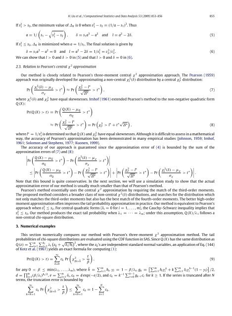
H. Liu et al. / Computational Statistics and Data Analysis 53 (2009) 853–856 855
1 > s2, the minimum value of ∆K is 0 when s 2
1 − s2 = (1/a − s1) 2 . Thus
� �
a = 1/ s1 − s 2
�
1 − s2 , δ = s1a 3 − a 2
If s 2
1 ≤ s2, ∆K is minimized when a = 1/s1. The final solution is given by
δ = s1a 3 − a 2 = 0 and l = a 2 − 2δ = 1/s 2
1 = c3
2 /c2
3
We can show that l > 0 and δ > 0 in (5) and that l > 0 and δ = 0 in (6).
2.3. Relation to Pearson’s central χ 2 approximation
and l = a 2 − 2δ. (5)
. (6)
Our method is closely related to Pearson’s three-moment central χ 2 approximation approach. The Pearson (1959)
approach was originally developed for approximating a non-central χ 2
l
Pr
where χ 2
l
Q (X):
� 2 χl (δ) − µχ
σχ
> t ∗
� � 2 χl ≈ Pr √
2l∗ ∗ − l∗
> t∗
2
(δ) distribution by a central χl∗ distribution:
�
, (7)
2 (δ) and χ ∗ have equal skewnesses. Imhof (1961) extended Pearson’s method to the non-negative quadratic form
Pr(Q (X) > t) = Pr
where l ∗ = 1/s 2
1
l
� Q (X) − µQ
σQ
� 2 χl ≈ Pr √
2l∗ ∗ − l∗
> t∗
> t ∗
�
�
�
= Pr χ 2
l∗ > l∗ + t ∗√ 2l∗ �
, (8)
2
is determined so that Q (X) and χl∗ have equal skewnesses. Although it is difficult to assess in a mathematical
way, the accuracy of Pearson’s approximation has been demonstrated in many empirical studies (Johnson, 1959; Imhof,
1961; Solomon and Stephens, 1977; Kuonen, 1999).
The accuracy of our approach is guaranteed since the approximation error of (4) is bounded by the sum of the
approximation errors of (7) and (8):
�
�
�
�Pr �
Q (X) − µQ
> t
σQ
∗
� � 2 χl (δ) − µχ
− Pr
> t
σχ
∗
��
���
�
�
≤ �
�Pr �
Q (X) − µQ
> t
σQ
∗
� � �� �
2 χl∗ − l∗ ��� �
− Pr √ > t∗ + �
2l∗ �Pr � � � 2
2
χl∗ − l∗
χl (δ) − µχ
√ > t∗ − Pr
> t
2l∗ σχ
∗
��
���
.
Note that this bound is quite conservative. In the next section, we will use a simulation study to show that the actual
approximation error of our method is usually much smaller than that of Pearson’s method.
Pearson’s method essentially uses the central χ 2 approximation by requiring the match of the third-order moments.
The proposed method considers a broader class of non-central χ 2 (δ) distributions, and searches for the distribution which
not only matches the third-order moments but also has the best match of the fourth-order moments. The better high-order
moment approximation often improves the tail probability approximation in practice. Our method is equivalent to Pearson’s
approach when s 2
1 ≤ s2. For central quadratic forms (δi = 0 for i = 1, . . . , m), the Cauchy–Schwarz inequality implies that
s 2
1 ≤ s2. Our method produces the exact tail probability when λ1 = · · · = λm; under this assumption, Q (X)/λ1 follows a
non-central chi-square distribution.
3. Numerical examples
This section numerically compares our method with Pearson’s three-moment χ 2 approximation method. The tail
probabilities of chi-square distributions are evaluated using the CDF function in SAS. Since Q (X) has the same distribution as
Q (z) = �m �hi i=1 j=1 λi
�
zij + √ �2, δi/hi where the zij’s are independent standard normal variables, an application of Eq. (144)
of Kotz et al. (1967) yields an exact formula for computing (1):
∞�
�
Pr(Q (X) > t) = ck Pr χ 2
�
t
> , (9)
2k+˜h β
k=0
for any 0 < β ≤ min(λ1, . . . , λm), where ˜h = � m
i=1 hi, γi = 1 − β/λi, gk = �� m
i=1
hiγ k
i + k � m
i=1
k−1
δiγi (1 − γi) � /2,
d = � m
i=1 (β/λi) h i/2 , e = � m
i=1 δi, c0 = d exp(−e/2), and ck = k −1 � k−1
r=0 gk−rcr for k ≥ 1. If the series is truncated after N
terms, the truncation error is bounded by
∞�
�
ck Pr χ 2
�
t
> ≤
2k+˜h β
∞�
ck = 1 −
k=N+1
k=N+1
N�
ck.
k=1