b) NMR: prediction of molecular alignment from structure

© 2008 

Nature 

Publishing 

Group 

http: 

/ / www. 

nature. 

com/ 

natureprotocols 

NMR: prediction of molecular alignment from 

structure using the PALES software 

Markus Zweckstetter 

Department for NMR-Based Structural Biology, Max Planck Institute for Biophysical Chemistry, Am Fassberg 11, 37077 Goettingen, Germany. Correspondence should be 

addressed to M.Z. (mzwecks@gwdg.de). 

Published online 27 March 2008; doi:10.1038/nprot.2008.36 

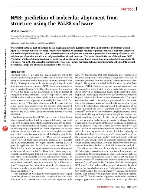
Orientational restraints such as residual dipolar couplings promise to overcome many of the problems that traditionally limited 

liquid-state nuclear magnetic resonance spectroscopy. Recently, we developed methods to predict a molecular alignment tensor and 

thus residual dipolar couplings for a given molecular structure. This provides many new opportunities for the study of the structure 

and dynamics of proteins, nucleic acids, oligosaccharides and small molecules. This protocol details the use of the software PALES 

(Prediction of AlignmEnt from Structure) for prediction of an alignment tensor from a known three-dimensional (3D) coordinate file 

of a solute. The method is applicable to alignment of molecules in many neutral and charged orienting media and takes into account 

the molecular shape and 3D charge distribution of the molecule. 

INTRODUCTION 

Structural studies of proteins and nucleic acids are critical for 

understanding biological processes at the molecular level. With the 

ability to determine atomic resolution structure, dynamics and 

folding of biological macromolecules in semiphysiological conditions, 

nuclear magnetic resonance (NMR) has become an eminent 

tool in structural biology 1 . Traditionally, structure determination 

by NMR has relied on the measurement of a large number of 

semiquantitative local restraints. The most important of these is the 

1 H– 1 H nuclear overhauser effect (NOE), which provides distance 

information for pairs of protons separated by less than B5 A ˚ .The 

accuracy of the NOE-derived distance usually decreases with the 

actual value of the distance because the precision of the measured 

intensity decreases with longer distance. Due to the strictly local 

nature of the NOE, several questions become difficult to answer 

with NMR. 

Residual dipolar couplings (RDCs) can be observed in solution 

when a molecule is aligned with the magnetic field: either as a result 

of its own magnetic susceptibility anisotropy, caused by an anisotropic 

environment such as an oriented liquid crystalline phase or 

an anisotropically compressed gel. When alignment can be kept 

sufficiently weak, the NMR spectra retain the simplicity normally 

observed in regular isotropic solution, while allowing quantitative 

measurement of a wide variety of RDCs, even in macromolecules 

2,3 . Several dilute liquid crystalline media are now available 

and RDC measurements are highly efficient, making RDCs a 

generally applicable tool for NMR structure determination 4,5 . 

RDCs describe the orientation of internuclear vectors with respect 

to the external magnetic field 6,7 . Thus, they contain long-range 

orientational information that can overcome many of the limitations 

of the traditional NMR structure determination process. For 

example, RDCs can be used to refine structures determined by 

conventional methods 8 , solve structures directly 9 ,validatestructures 

10 , analyze relative orientations of molecular fragments or 

domains 11 , study dynamic effects 12 or characterize intrinsically 

disordered proteins 13,14 . 

Weak alignment of biological macromolecules in dilute liquid 

crystalline phases or anisotropically compressed gels can result 

from steric or electrostatic interactions with the alignment med- 

PROTOCOL 

ium. We demonstrated that both magnitude and orientation of 

the steric component of the molecular alignment tensor can be 

accurately predicted from the molecule’s three-dimensional (3D) 

shape 15 . The approach is called Prediction of ALignmEnt from 

Structure (PALES). Further on, we and others demonstrated that 

the approach is not restricted to nearly neutral alignment media. 

RDCs observed for proteins and nucleic acids dissolved in dilute 

suspensions of the highly negatively charged filamentous phage can 

be predicted from the 3D structure of a biomolecule 16,17 . A highly 

oversimplified model, one which approximated the electrostatic 

interaction between a solute and an ordered phage particle (as that 

between the solute charge topography and the electric field of the 

phage), predicted the solute’s alignment tensor with reasonable 

accuracy 17 . Recently, we showed that the simple electrostatic model 

is also applicable to partial alignment at low pH and in surfactant 

liquid crystalline systems 18 . In the case of uniformly charged 

systems, as nucleic acids aligned in negatively charged bacteriophage, 

the rhombicity and orientation of the alignment tensor can 

also be predicted using only a steric interaction model 17,19 .The 

steric interaction model might be further simplified such that the 

molecule is not represented in atomic detail, but rather by its 

hydrodynamic shape 20 , gyration tensor 19 , moment of inertia 21 or 

the problem is solved analytically 22 . Fast and simple analytical 

solutions allow incorporation of alignment prediction into molecular 

dynamics simulations. However, these predictions are less 

accurate than those obtained by the PALES simulation method. 

The ability to predict a molecular alignment tensor and thus 

RDCs for a given molecular structure opens the door to many new 

opportunities: for example, it can be used to differentiate between 

monomeric and homodimeric states 15 ; validate 3D structures of 

protein complexes 23 ; determine the relative orientation of protein 

domains 24 ; classify protein-fold families on the basis of unassigned 

NMR data 25 ; refine nucleic acid structures 26 ; determine the global 

structure of branched nucleic acids 27 ; characterize the conformation 

of intrinsically disordered proteins 28–30 ; and analyze dynamic 

systems such as multidomain proteins, nucleic acids and oligosaccharides 

31,32 . The electrostatic alignment model offers additional 

unique opportunities, such as distinction between parallel and 

NATURE PROTOCOLS | VOL.3 NO.4 | 2008 | 679

© 2008 

Nature 

Publishing 

Group 

http: 

/ / www. 

nature. 

com/ 


PROTOCOL 

antiparallel arrangements of homodimeric systems 33 ,theidentification 

of domain swaps in oligomeric proteins (S. Rumpel and 

M.Z., personal communication) or the analysis of nonspecific 

protein–DNA interactions 34 . 

Here, I present a detailed protocol for prediction of an alignment 

tensor for a given 3D molecular structure using PALES. 

The PALES software 

Prediction of molecular alignment is at the heart of the PALES 

program. In addition, many other functions for analysis of RDCs 

are available in PALES. This includes the estimation of axial and 

rhombic components of molecular alignment tensors in the 

absence of structural information 35,36 , back-calculation of alignment 

tensors from RDCs using well-defined molecular fragments 

37 , analysis of uncertainty in back-calculated tensors 38 ,as 

well as efficient handling of dipolar couplings, alignment tensors 

and corresponding ProteinDataBank (PDB) files. The PALES software 

is fully applicable to proteins 15 , nucleic acids 17 and oligosaccharides. 

All tasks can be performed on the command line and 

more complex projects can be set up as scripts. Use of default 

parameters allows concise argument lists. For example, ‘pales -pdb 

ref.pdb’ performs a PALES shape-prediction for the molecular 

structure recorded in ‘ref.pdb’, using an infinite wall model with a 

sample volume fraction of 5% and a diameter of the liquid crystal 

particle of 40 A ˚ (see below for further details). Alternatively, a 

graphical user interface is available that integrates the various RDC 

analysis tools with the text editor Vi, the 2D plotting program 

Grace, and the molecular graphics program Rasmol. 

Molecular alignment 

The average orientation of a weakly aligned macromolecule with 

respect to the magnetic field is described by a second-rank tensor S, 

with a maximum of five independent elements 7 . The elements of 

this traceless tensor are 

dij4 

ði; j ¼ x; y; z; dij ¼ 1fori¼ j; dij ¼ 0fori6¼ jÞ 

Sij ¼1=2o3 cosyi cos yj 

where yi is the angle between the molecular axis i and the 

magnetic field, and the brackets o4 denote time or ensemble 

averaging. The eigenvectors and eigenvalues of this real and 

symmetric matrix S correspond to the axes, the magnitude and 

the rhombicity of the molecular alignment tensor. This tensor can 

be related to the coordinate system of the molecule by a 3D Euler 

rotation that accomplishes the diagonalization of the ordering 

matrix. 

For a pair of spin-1/2 nuclei P and Q, separated by a distance rPQ, 

the d PQ dipolar coupling is related to the average orientation of the 

whole molecule by 

d PQ ¼ SLS m 0g Pg Qh=ð8p 3 or 3 PQ 4Þ 

Si;j Sij cos f PQ 

i 

cos f PQ 

j 

S LS is the Lipari–Szabo generalized order parameter, which scales 

d PQ for the effect of fast librations of the internuclear vector 39 . g P 

and gQ are the gyromagnetic ratios, h is Planck’s constant, m0 is the 

magnetic permeability of vacuum, rPQ is the internuclear distance 

and fi PQ is the angle between the P–Q internuclear vector and the 

680 | VOL.3 NO.4 | 2008 | NATURE PROTOCOLS 

ð1Þ 

ð2Þ 

ith molecular axis. In the principal axis frame (superscript d), 

equation (2) can be rewritten as 

d PQ ¼ðyPQ; f PQÞ ¼1=2 D PQ 

max ½Aað3 cos 2 yPQ 1Þ 

+3=2 Ar sin 2 yPQ cosð2f PQÞŠ 

Aa ¼ Szz d is the axial component of the alignment tensor and 

Ar ¼ 2/3 (Sxx d Syy d ) is its rhombic component with |Szz d | 4 |Syy d | 

Z|Sxx d |, yPQ and fPQ being cylinder coordinates defining the 

vector orientation relative to this tensor; D PQ max ¼ SLS m0gPgQh/ 

(8p 3 hrPQ 3 i) is the dipolar interaction value for the P–Q internuclear 

vector. 

Back-calculation of the alignment tensor 

If well-defined structures of complete macromolecules, their domains 

or smaller fragments thereof are available, an alignment tensor S can be 

calculated from the observed dipolar couplings (‘-bestFit’ modulein 

PALES). All five independent elements of the alignment matrix can be 

determined, provided a minimum of five experimental RDCs are 

available. More couplings may be required if any pair of internuclear 

vectors are nearly parallel to each other, or if more than three vectors are 

located in a single plane. Two approaches for best-fitting an alignment 

tensor to experimental RDCs are in common use: iterative least-squares 

minimization and singular value decomposition (SVD). SVD obtains a 

solution for the linear equation system formed by equation (3) by 

calculating the Moore–Penrose inverse of the directional cosine 

matrix 37 . The transformation returns an alignment tensor for which 

calculated RDCs have the least-squares deviation from the observed 

ones. It is more stable than iterative least-squares minimization and 

requires only a minimum of five RDCs. Therefore, SVD is particularly 

useful when only a limited set of dipolar couplings are available. 

If previous knowledge of any of the alignment tensor parameters 

is available, an iterative least-squares procedure (Levenberg– 

Marquardt in the RDC software PALES) that minimizes the 

differences between experimentally observed d i PQ (exp) values and 

those back-calculated from equation (3) becomes the method of 

choice 40 . In this method, any of the five independent alignment 

parameters may be held fixed. Under these conditions, if threefold 

or higher symmetry exists, the rhombic component is known to be 

zero and the dimensionality of the search can be reduced to four. 

Evaluation of alignment tensor accuracy 

To estimate the uncertainty in alignment tensor values obtained by 

best-fitting experimental RDCs to a given structure, the backcalculation 

may be repeated many times (B1,000 times), but 

each time with different Gaussian noise added to the experimental 

RDCs. In this so-called Monte-Carlo approach, only those solutions 

are accepted for which all back-calculated RDCs are within a 

given margin of the original experimental dipolar couplings. This 

procedure works quite well when the error in the data is dominated 

by the random measurement error in the dipolar coupling. To 

indirectly account for uncertainties in the structure, it was suggested 

to set the amplitude of the added noise to 2–3 times higher 

than the measurement uncertainty 37 . In the program PALES, this 

approach is optimized by iteratively adjusting the amplitude of the 

noise added to the dipolar couplings such that an adjustable 

fraction of the solutions are accepted when using an acceptance 

margin that is twofold larger than the r.m.s. amplitude of the 

added noise. 

ð3Þ

© 2008 

Nature 

Publishing 

Group 

http: 

/ / www. 

nature. 

com/ 


When structural noise dominates the error in the SVD fit, the 

noise is effectively distributed very differently for different data 

points. Therefore, a second method for evaluating the uncertainty 

in the alignment tensor, the so-called ‘structural noise Monte-Carlo 

method’, was implemented 38 . In the ‘structural noise Monte-Carlo 

method’, noise is added to the original structure with an amplitude 

to match the root mean square deviation (RMSD) between the 

experimental and back-calculated RDCs. The noise is introduced 

into the structure by slightly reorienting the selected vector orientations 

in a random manner such that the deviations between the 

original and final vectors are described by a Gaussian cone-shaped 

distribution, with a standard deviation scone and a relative probability 

of sin(b)exp( b 2 /scone 2 ) for an angle b between the original 

and modified orientation. The spread in the alignment parameters 

obtained for these noise-corrupted structures, when using the 

coupling constants calculated for the original structure (i.e., yielding 

a perfect fit if no structural noise were added), then provides 

another unbiased measure for the spread in the alignment parameters. 

On average, the Losonczi Monte-Carlo method, when 

implemented in the way described above (‘-mcDc’ module in 

PALES), and the structural noise Monte-Carlo method (‘-mcStruc’ 

module in PALES) yield uncertainties that are quite similar to one 

another. However, some differences can occur when considering 

small fragments and the ‘structural noise Monte-Carlo method’ is 

recommended, in general. 

Prediction of molecular alignment from the 3D shape of a 

molecule 

When the interaction between the macromolecular solute and the 

nematogenic particles is predominantly steric in nature, the alignment 

tensor can be accurately predicted from the solute’s 3D shape 

(‘-stPales’ module in PALES) 15 . This is quite different from the 

procedures described above where the alignment tensor is derived 

from a fit of experimental RDCs to a known structure. Although 

the steric prediction approach by definition can never exceed the 

goodness of fit obtained by the SVD method, it offers different 

attractive features, as it predicts molecular ordering and RDCs from 

a simple steric obstruction model. 

The steric obstruction algorithm consists of a one-dimensional 

translational grid search combined with uniform sampling of 

molecular orientations (Fig. 1a): the nematogen is approximated 

by an infinite wall (bicelles; ‘-bic’ parameter in PALES) or infinite 

cylinder (Pf1 bacteriophage; ‘-pf1’ parameter in PALES), oriented 

parallel to the magnetic field (z axis). The center of gravity of the 

solute is moved on a one-dimensional grid, with a spacing between 

grid points of 0.2 A ˚ , away from the surface of the liquid crystal 

model (‘-dGrid’ parameter in PALES). At each step, a set of 2,196 

different molecular orientations is sampled. These 2,196 orienta- 

Figure 1 | Schematic outline of the PALES algorithm for the prediction of 

molecular alignment in the case of steric obstruction. (a) One-dimensional 

translational grid (black diamonds) in front of an infinite wall or cylinder 

(blue rectangle) on which the molecule is moved during the simulation. At 

each position, different orientations of the molecule are uniformly sampled 

(right panel). (b) When the molecule is close to the surface of a liquid crystal 

particle (blue rectangle), it clashes in certain orientations (shown in red), 

whereas other orientations are sterically allowed (shown in green). When the 

molecule is far away from the liquid crystal particle, all orientations are 

equally probable. For details, see the section ‘Prediction of molecular 

alignment from the 3D shape of a molecule’. 

tions are obtained in a two-step procedure. First, the z axis of the 

molecule samples 122 points (minimum number of points) on a 

unit sphere that were determined by a double cubic lattice method 

(‘-dot’ parameter in PALES) 41 . This provides a highly uniform 

sampling of the sphere. In a second step, the molecule is rotated 

around the z axis in steps of 201 (‘-digPsi’ parameter in PALES). 

For each orientation, the program evaluates whether the solute 

sterically clashes with the nematogen, that is, if any of the solute atoms 

has a coordinate within the wall or cylinder model. For example, for a 

disk-shaped nematogen and a rod-shaped solute molecule, a larger 

fraction of molecules oriented orthogonal to the disks will be 

obstructed than those molecules parallel to the disk surface, resulting 

in net ordering of the remaining nonobstructed molecules (Fig. 1b). 

For these nonobstructed orientations/positions, an alignment matrix 

S is calculated according to equation (1). The overall molecular 

alignment tensor S mol is simply the linear average over all nonexcluded 

S matrices. Using periodic boundary conditions, sampling is 

restricted to distances r between the solute center of gravity and the 

center of the bilayer or cylinder for which r o d/(2Vf) (wall model), 

or r o d/(4Vf) 1/2 (cylinder), where d (two times the ‘-rM’ parameter 

in PALES) is either the wall thickness (40 A ˚ for bicelles) or the 

cylinder diameter (67 A ˚ for Pf1) and Vf is the nematogen volume 

fraction. The imperfect alignment of liquid crystals is taken into 

account by multiplication of S mol with the order parameter of the 

liquid crystal (‘-lcS’ parameter in PALES). Note that the biomolecule 

is represented in atomic detail in PALES simulations. 

Prediction of molecular alignment from the 3D charge 

distribution and shape of a molecule 

The obstruction model only includes a steric term, and orientations 

of all nonobstructed orientations and positions of the protein 

are weighted equally. In the case of a charged liquid crystal as 

bacteriophage Pf1 (ref. 42), this simple model fails. Considering 

that bacteriophage is highly negatively charged (–0.47 e nm 2 

average surface charge density), it becomes clear that electrostatic 

interactions between protein molecules and liquid crystal particles 

cause the probabilities of sterically allowed solute orientations to 

depend strongly on this orientation and the distance from the 

liquid crystal particle (Fig. 2). 

a 

b 

PROTOCOL 


© 2008 

Nature 

Publishing 

Group 

http: 

/ / www. 

nature. 

com/ 


PROTOCOL 

To take into account electrostatic effects, each nonexcluded 

S matrix is weighted according to its Boltzmann probability, PB, 

after calculating the corresponding electrostatic potential of the 

solute (‘-elPales’ module in PALES). Continuum electrostatic 

theory43 is used for calculating the electrostatic interaction energy: 

the solute is embedded in a dielectric medium containing 

excess ions in addition to the counter ions neutralizing the solute 

and nematogen. The nonlinear Poisson–Boltzmann (PB) equation 

is used to derive the electrostatic potential44,45 . Even within 

the simplifications of a continuum description, calculations of 

the electrostatic potentials would require solving a full 3D electrostatics 

problem for each distance and orientation of the solute with 

respect to the surface of the charged liquid crystal particle. Instead, 

we further simplify the problem by treating the solute as a particle 

in the external field of the liquid crystal. Moreover, we assume 

that the nematogen carries a uniform charge density (‘-chSurf’ 

parameter in PALES) instead of discrete surface charges. 

The nonlinear 3D PB equation is then solved only once, in the 

absence of the solute, yielding an electrostatic potential j(r). The 

distance- and orientation-dependent electrostatic free energy of 

the protein comprising partial charges qi at positions ri are then 

approximated by 

DGelðr; OÞ ¼Si qi f½riðr; OÞŠ: 

The Boltzmann factor PB ¼ exp[ DGel(r,O)/kBT] provides relative 

electrostatic weights when averaging the individual alignment 

tensors, derived for each orientation and distance, to yield an 

overall solute alignment tensor: 

Z 

Z 

A mol 

ij 

¼ 

AijPBðr; OÞ dr dO= 

PBðr; OÞ dr dO: ð5Þ 

MATERIALS 

EQUIPMENT 

.Hardware: Computer running Unix, Linux, Mac OS X or Windows 

operating system 

.Software: PALES is available to academic users for free download from 

http://www.mpibpc.mpg.de/groups/griesinger/zweckstetter/_links/ 

software_pales.htm 

.Input files (see also Supplementary Data): 

. 3D coordinate file; most standard PDB files are recognized, including 

multiple chain and segment molecules 

P B = exp[–∆G e1 (r,Ω)/k B T ] 

Figure 2 | Schematic outline of the PALES algorithm simulating weak ordering 

of molecules in charged alignment media. A protein is embedded in the 

external electrostatic field of the liquid crystal. Electrostatic interactions 

between the protein molecule and a liquid crystal particle cause the 

probabilities of sterically allowed solute orientations to depend strongly on 

this orientation and the distance from the liquid crystal particle. For details, 

see the section ‘Prediction of molecular alignment from the 3D charge 

distribution and shape of a molecule’. 

For a flat surface (‘-bic’ parameter in PALES), an analytical solution 

of the nonlinear PB equation exists 44,45 . For uniformly charged 

cylinders such as bacteriophage (‘-pf1’ parameter in PALES), the 

method of Stigter 46 is used assuming symmetric monovalent ions 

and vanishing potential at infinity. 

Input and output files used in the protocol can be found in the 

Supplementary Data online. In addition, a shell script is provided 

for running the PALES tasks outlined in the protocol. 

. RDC table (Table 1); required for best-fitting RDCs to a molecular 

structure (‘-bestFit’ module of PALES), but not essential for prediction 

of molecular alignment (‘-stPales’ and‘-elPales’ modules of PALES) 

. For prediction of molecular alignment induced by uniformly charged 

cylinders (‘-elPales -pf1’): 

. File containing the charges of the molecule (Table 2; see also Step 14). 

. File containing the electrostatic potential (Table 3). 

PROCEDURE 

Preparation of input 

1| Prepare the coordinate file or download a 3D structure from the PDB (http://www.rcsb.org/pdb) (e.g.,‘pdb1ubq.ent’). When 

multiple models are present in the coordinate file, select one and remove the others by using your preferred editor. Remove 

unwanted parts of the structure (or use PALES selection flags (see Step 3)). If the PDB file does not contain protons, add 

protons to the structure using, for example, the program Reduce (http://kinemage.biochem.duke.edu/software/reduce.php) 

(e.g., ‘pdb1ubqH.ent’; see Supplementary Data to know how to add protons to a crystal structure using the program Reduce). 

If you are only interested in prediction of the molecular alignment tensor (and not RDCs), go to Step 9. 

m CRITICAL STEP For alignment prediction, all atoms in the PDB file will be used (including pseudo atoms such as ‘ANI’), 

when no appropriate selection command line arguments are specified. 

2| Prepare the RDC input table (e.g., ‘dObs.tab’; Supplementary Data). The table must include a ‘VARS’ line and a 

‘FORMAT’ line that label the corresponding columns of the table and define its data type, respectively (Table 1). Lines with a 

‘#’ sign as first character as well as empty lines are ignored. The table must include columns for residue ID, three-character 

682 | VOL.3 NO.4 | 2008 | NATURE PROTOCOLS

© 2008 

Nature 

Publishing 

Group 

http: 

/ / www. 

nature. 

com/ 


TABLE 1 | Example of a PALES RDC input table (selection of 1H-15N RDCs observed in the 76-residue protein ubiquitin weakly aligned in bicelles) 2 . 

VARS RESID_I RESNAME_I ATOMNAME_I RESID_J RESNAME_J ATOMNAME_J D DD W 

FORMAT %5d %6s %6s %5d %6s %6s %9.3f %9.3f %.2f 

3 ILE N 3 ILE H 8.271 1.000 1.00 

4 PHE N 4 PHE H 10.489 1.000 1.00 

5 VAL N 5 VAL H 9.871 1.000 1.00 

6 LYS N 6 LYS H 9.152 1.000 1.00 

7 THR N 7 THR H 3.700 1.000 1.00 

13 ILE N 13 ILE H 6.947 1.000 1.00 

14 THR N 14 THR H 9.713 1.000 1.00 

15 LEU N 15 LEU H 9.851 1.000 1.00 

16 GLU N 16 GLU H 1.909 1.000 1.00 

17 VAL N 17 VAL H 0.041 1.000 1.00 

18 GLU N 18 GLU H 10.513 1.000 1.00 

20 SER N 20 SER H 4.071 1.000 1.00 

21 ASP N 21 ASP H 2.119 1.000 1.00 

23 ILE N 23 ILE H 9.098 1.000 1.00 

25 ASN N 25 ASN H 2.948 1.000 1.00 

26 VAL N 26 VAL H 8.892 1.000 1.00 

residue name and the atom name for both atoms that are involved in the dipolar coupling. Segment ID and Chain ID are 

optional. The ‘D’ column gives the RDC value in Hz. Hetero- and homonuclear RDCs involving C, N, H, P and F atoms can be used 

simultaneously. When no experimental RDCs are available, any nonzero dummy values can be entered (in this case, go directly 

to Step 9). The ‘DD’ column gives an indication of the experimental RDC error (relative to 1 D NH). The weight column ‘W’ is used 

for comparison of input and calculated RDCs (e.g., for calculation of root-mean-square deviations between input and calculated 

RDCs) and should be normalized to 1 D NH according to the gyromagnetic ratios of the involved nuclei and the internuclear 

distance, that is, W( 1 D NH) ¼ 1.000, W( 1 D CC) B 5.05, W( 1 D NC) B 8.33, W( 1 D CH) B 0.48, W( 2 D HnC) B 3.33. Note that values 

in column ‘W’ do not influence best-fitting or prediction of 

TABLE 2 | Example of a PALES charge file for the 76-residue 

protein ubiquitin. 

1 Terminus Charge 0.711 

6 Default Charge 0.989 
























76 O Charge 0.491 

76 OXT Charge 0.491 

PROTOCOL 

molecular alignment tensors and therefore also not RDCs 

back-calculated from calculated/predicted alignment tensors. 

For best-fitting or prediction of molecular alignment, input 

and calculated RDCs are scaled automatically by the dipolar 

interaction value for a specific internuclear vector. For 

one-bond backbone RDCs, optimized values of the internuclear 

distance are used for calculation of the dipolar interaction 

value. For all other RDCs, internuclear distances are taken from 

the3Dcoordinatefile. 

m CRITICAL STEP The atom notation in the RDC table must 

match that of the PDB file. Check, in particular, the notation 

of amide protons (i.e., ‘H’ or ‘HN’). 

TABLE 3 | Part of a PALES input file that contains the values for the 

electrostatic potential. 

0.00 2.22 105 1.00E + 03 2.18 105 2.00E + 03 2.14 105 3.00E + 03 2.10 105 4.00E + 03 2.06 105 5.00E + 03 2.02 105 6.00E + 03 1.98 105 7.00E + 03 1.95 105 8.00E + 03 1.91 105 The first column specifies the distance from the surface of the alignment medium (in nm); the second 

column specifies the value of the electrostatic potential (in e kBT 1 ). Files containing the electrostatic 

potential of Pf1 phage at different salt concentrations can be downloaded from http://www.mpibpc. 

mpg.de/groups/griesinger/zweckstetter/_links/software_pales.htm. 


© 2008 

Nature 

Publishing 

Group 

http: 

/ / www. 

nature. 

com/ 


PROTOCOL 

TABLE 4 | Parameters reported by PALES in RDC output files (see Supplementary Data). 

Parameter Definition 

DATA SAUPE Five independent values (S(zz), S(xx-yy), S(xy), S(xz), S(yz)) of the alignment tensor7 DATA IRREDUCIBLE Irreducible representation of the alignment tensor47 DATA IRREDUCIBLE 

GENERAL_MAGNITUDE 

General magnitude of the alignment tensor4,47 DATA MAPPING Sauson–Flamsteed coordinates (i.e., x and y coordinates for the x, y and z axis of the alignment tensor) 

DATA MAPPING INV Sauson–Flamsteed coordinates of the inverted axes of the alignment tensor (relative to DATA MAPPING) 

DATA EIGENVALUES Eigenvalues (Sxx_d,Syy_d,Szz_d) of the alignment tensor (i.e., the values of the alignment tensor in the principal 

axis frame) 

DATA EIGENVECTORS Eigenvectors for diagonalization of the alignment tensor 

DATA Q_EULER_ANGLES Euler angles for rotation of the alignment tensor into the principal axis frame, that is, for diagonalization of the 

alignment tensor. Values are specified according to the definition used in quantum mechanics, that is, for clockwise 

rotation about the three independent axes z (angle ALPHA), y ¢ (angle BETA) and z 00 (angle GAMMA). Four different 

Euler angles are reported due to the fourfold degeneracy of alignment tensors 

DATA EULER_ANGLES Euler angles for rotation into the principal axis frame using a rotation about three dependent axes x (angle psi), 

y (angle theta) and z (angle phi). Two solutions are provided 

DATA Da Da ¼ 1 / 2 S d 

zz 

DATA Dr Dr ¼ 1 / 3 (S xx d S yy d ) 

DATA Aa Axial component of the alignment tensor Aa ¼ S d 

zz . 

DATA Ar Rhombic component of the tensor Ar ¼ 2 / 3 (S d 

xx S d 

yy ) 

DATA Da_HN Axial component (in Hz) of the alignment tensor normalized to the dipolar interaction constant of the one-bond NH 

internuclear vector (Da_HN ¼ 1 /2 D NH max Aa ¼ 1 /2 21585.19 Aa) 

DATA rhombicity Rhombicity R ¼ Ar/Aa of the alignment tensor (range: [0, 2 /3]) 

DATA N Number of RDCs used in the calculation 

DATA RMS Root-mean-square deviation between input and calculated RDCs 

DATA Chi2 w2 value between input and calculated RDCs 

DATA CORR R Pearson’s linear correlation coefficient between input and calculated RDCs (range: [ 1, 1]) 

DATA Q SAUPE RDC Q-factor calculated according to Q ¼ {Si¼1,..,N [d norm 

i (exp) di 

norm (calc)] 2 /N} 1/2 /Dr.m.s. ,withNbeing the 

number of measured and normalized couplings, d norm 

i (exp). Dr.m.s. refers to the root-mean-square value of RDCs for 

randomly distributed internuclear vectors. It can be calculated directly from experimental dipolar couplings 

Dr.m.s. ¼ [Si¼1,..,N (di norm ) 2 ] 1/2 (‘-qRms’ flag) or from the axial and rhombic component of the alignment tensor 

Dr.m.s. ¼ [2 (Da norm ) 2 (4 + 3R2 )/5] 1/2 ,withDa norm being the normalized axial component (‘-qDa’flag;thisisthedefault 

selection) 

DATA REGRESSION OFFSET Vertical offset of straight line fit to a comparison of input and calculated RDCs 

DATA REGRESSION SLOPE Slope of straight line fit to a comparison of input and calculated RDCs 

DATA REGRESSION BAX 

SLOPE 

Average of slope obtained from straight line fits of y ¼ ax + b and x ¼ cy + d, thatis,BAXSLOPE¼0.5 (a + 1/c) 

Best-fitting experimental RDCs to 3D structure 

3| Run PALES to best-fit experimental RDCs to the 3D structure by executing the following command on the command line: 

PALES -bestFit -pdb pdb1ubqH.ent -inD dObs.tab -outD dCalc.Svd.tab 

m CRITICAL STEP Include the ‘-bestFit’ flag. 

? TROUBLESHOOTING 

4| Check if the RDC table and PDB file were properly read in by PALES. PALES reports some information (including errors and 

warnings on the command line as stderr). The first two lines indicate which PDB file and RDC table were provided as input, how 

many residues and atoms were recognized in the PDB file and how many residues and couplings were there in the RDC table. The 

first line starting with ‘REMARK’ reports how many atom pairs (RDCs) in the input table could be matched to internuclear vectors 

in the PDB file (i.e., how many RDCs will be used for best-fitting). The second ‘REMARK’ line reports the selection criteria applied 

to the PDB file. 



© 2008 

Nature 

Publishing 

Group 

http: 

/ / www. 

nature. 

com/ 


PROTOCOL 

5| Inspect the output file (e.g., ‘dCalc.Svd.tab’). Determine the degree of alignment from the norm of the irreducible 

representation of the alignment tensor (‘DATA IRREDUCIBLE GENERAL_MAGNITUDE’) or the magnitude of its largest eigenvalue 

(‘Szz_d’). ‘Szz_d’ normalized to 1DNH can be found in the ‘DATA Da_HN’ parameter. ‘DATA Da_HN’ is generally in the range 

B5–20 Hz. Using ‘DATA Da_HN’ or ‘Szz_d’ can be misleading in the case of high rhombicity. Evaluate the orientation of the 

alignment tensor that is described by three Euler angles ‘ALPHA’(clockwiserotationaroundz,leadingtonewsystemx¢,y¢,z¢), ‘BETA’ 

(clockwise rotation around y’, leading to new system x00 ,y00 ,z00 ) and ‘GAMMA’ (clockwise rotation around z00 ). Four equivalent Euler 

orientations are reported due to the sign ambiguity of the eigenvectors. Check the RDC statistics, that is, did PALES use the number 

of RDCs you supplied (parameter ‘DATA N’), what is Pearson’s correlation coefficient between experimental and back-calculated 

RDCs (‘DATA CORR R’), is the dipolar coupling Q value sufficiently low (‘DATA Q SAUPE’; Q values for high-resolution structures range 

from 17% when comparing experimental ubiquitin dipolar couplings with its 1.8-A˚ X-ray structure to 11% when comparing dipolar 

couplings for the third IgG-binding domain of streptococcal protein G with its 1.1-A˚ X-ray structure), are there systematic errors 

in the experimental RDCs that cause an offset (‘DATA REGRESSION OFFSET’) between experimental and back-calculated RDCs or a 

slope (‘DATA REGRESSION SLOPE’) deviating from one (further details can be found in Table 4). 

m CRITICAL STEP For high-resolution X-ray structures (solved at a resolution of 2.5 A˚ or better), Pearson’s correlation coefficient 

between experimental and calculated couplings (‘DATA CORR R’) is expected to be above 0.9. 


6| Refine the RDC input table. Search the column ‘D_DIFF’, which lists the difference between experimental and calculated RDCs, for 

values that significantly exceed the values obtained for most of the other residues. Check the NMR spectra and determine, if signal 

overlap or low signal-to-noise ratio is responsible for the large deviations. Under these circumstances, remove the corresponding RDC 

values from the input table (e.g., by marking them out with a ‘#’ sign in the beginning of the line) and repeat Steps 3–6. 

7| Visualize the orientation of the alignment tensor (optional). Rerun PALES by including the ‘-pdbRot’ flag, that is, ‘PALES 

-bestFit -pdb pdb1ubqH.ent -inD dObs.tab -outD dCalc.Svd.tab -pdbRot rot.pdb -nosurf –H’. 

In the PDB output file (e.g., ‘rot.pdb’), the molecule will be rotated such that the alignment tensor is parallel to the laboratory 

frame. Load the PDB output file into any molecular visualization program and activate the axes of the laboratory frame. 


8| Determine the uncertainty in the alignment tensor parameters. Execute PALES with the command line flag ‘-mcStruc’ and 

set the number of Monte Carlo steps to B1,000 (‘-map 1000’): 

PALES -bestFit -pdb pdb1ubqH.ent -inD dObs.tab -outD dCalc.McStruc.tab -mcStruc -map 

1000 -outDa tMag.tab -outMap tCoor.tab -outAng tAng.tab -outA tSaupe.tab 

Alignment tensor parameters for each Monte Carlo step are written to files by specifying the ‘-outDa’, ‘-outMap’, 

‘-outAng’ and ‘-outA’ flags. Extract the uncertainty in the alignment tensor parameters from the ‘DATA STATISTICS 

MAPPING’ fields in the output file (e.g., ‘dCalc.McStruc.tab’). 

m CRITICAL STEP The RDC weight factors (in the column ‘W’ of the RDC input table) must have the correct values (see Step 2). 

Prediction of molecular alignment from the 3D shape of a biomolecule 

9| Perform the alignment prediction using the steric interaction model. When no RDCs are available (either experimental RDCs 

or dummy values), execute one of the following commands on the command line. 

PALES -pdb pdb1ubqH.ent -H 

If you have prepared an RDC input table (e.g., ‘dObs.tab’), execute 

PALES -pdb pdb1ubqH.ent -H -inD dObs.tab 

If you want to store the output into a file (e.g.,‘dCalc.Steric.tab’), execute 

PALES -pdb pdb1ubqH.ent -H -inD dObs.tab –outD dCalc.Steric.tab 

This is identical to executing 

PALES -stPales -bic -wv 0.05 -pdb pdb1ubqH.ent -inD dObs.tab -outD dCalc.Steric.tab -H 

The ‘-bic’ flag selects the infinite wall model (e.g., when using bicelles). For the infinite cylinder model, ‘-bic’ should 

be replaced by ‘-pf1’. The orientation of the bilayer/cylinder relative to the magnetic field cannot be changed. Specify the 

concentration of the liquid crystalline phase (‘-wv 0.05’ in g ml 1 ). 

m CRITICAL STEP Inclusion of protons (‘-H’ flag) can significantly influence the predicted alignment tensor. 


10| Evaluate the results of alignment prediction in the output file (e.g., ‘dCalc.Steric.tab’). Control the simulation parameters 

(lines starting with ‘DATA PALES’). The default value of the order parameter of the liquid crystal is 0.8 (‘DATA PALES LC_ORDER’). 

The magnitude of alignment (‘DATA Da_HN’) scales linearly with the concentration of the dilute liquid crystalline medium. 

Inspect the various quality measures of calculated RDCs such as root-mean-square deviation (‘DATA RMS’), Pearson’s linear 

correlation coefficient (‘DATA CORR R’) and RDC quality factor (‘DATA Q SAUPE’). 



© 2008 

Nature 

Publishing 

Group 

http: 

/ / www. 

nature. 

com/ 


PROTOCOL 

11| Test the influence of variations in the 3D structure. Discard flexible parts of the structure (in this case residues 73–76) by 

manually editing the PDB file or by using PALES PDB selection flags, for example, 

PALES -stPales -bic -wv 0.05 -pdb pdb1ubqH.ent -inD dObs.tab -outD dCalc.Steric.tab -H -r1 

1 -rN 72 

Repeat the procedure with differing selections (e.g., ‘-r1 2 -rN 72’ or ‘-r1 1 -rN 74’) and evaluate the influence on 

alignment prediction. 

m CRITICAL STEP Especially with nearly spherical and small proteins, ill-defined/flexible termini can strongly influence the simulation. 


12| Test the convergence of the alignment prediction. For most molecules, default simulation parameters give reasonable 

results. Rerun PALES with increased resolution of the orientational (‘-digPsi’ and ‘-dot’) and translational grid 

‘-dGrid’ (in A˚) and a modified value for the uniform atom radius ‘-rA’ (in A˚) (see this section). Additionally, the selection 

of surface accessible atoms can be suppressed by the inclusion of the ‘-nosurf ’ flag (i.e., all atoms are taken into account). 

PALES -stPales -bic -wv 0.05 -pdb pdb1ubqH.ent -inD dObs.tab -outD dCalc.StericHR.tab -H 

-dGrid 0.1 -dot 133 -digPsi 36 -rA 1.9 -nosurf 

Compare the correlation between experimental and predicted couplings obtained for different simulation parameters 

(e.g., ‘DATA CORR R’ values in ‘dCalc.Steric.tab’ and ‘dCalc.StericHR.tab’). 

m CRITICAL STEP The molecular alignment prediction can never exceed the goodness of fit obtained by the SVD method. 

13| Compare the predicted orientation of alignment with that obtained from best-fitting RDCs. Extract the alignment tensor 

values (‘DATA SAUPE’) from the output file obtained by SVD (e.g., ‘dCalc.McStruc.tab’ in Step 8) and from the output file obtained 

by alignment prediction (e.g., ‘dCalc.Steric.tab’ in Step 11). Run PALES with the following flags 

PALES -anA -inS1 -4.3110e-04 1.5328e-04 -2.0599e-04 -4.8808e-04 -3.9182e-04 -inS2 

-3.9955e-04 -6.7056e-05 -3.1392e-04 -7.6731e-04 -4.0968e-04 -outA dCp.Saupe.tab 

In the output file (e.g., ‘dCp.Saupe.tab’), seek out the following parameters that describe the angles between the axes of the 

two tensors in three and five dimensions, as well as their collinearity, respectively: ‘DATA ANGLE_3D_AXES (X/Y/Z)’, ‘DATA 

ANGLE_5D_SPACE’ and ‘DATA COLL_5D’. Further details regarding these parameters can be found in ref. 47. 

m CRITICAL STEP Saupe values have to be given in the order S(zz), S(xx-yy), S(xy), S(xz) and S(yz). 

Prediction of molecular alignment from the surface charge distribution and molecular shape 

14| Set up the file listing the charges of the molecule (Table 2). Generate an initial version of this file (e.g., ‘charge.tab’) by 

running PALES: 

PALES -anPdb -pdb pdb1ubqH.ent -outPka charge.tab -el -outP out.PdbSim.tab -pkaDef -pH 7.0 

Display the charge file (e.g., ‘charge.tab’) using your preferred editor. The file contains four columns. Columns 1–4 specify the 

residue number, the name of the atom where the charge is located, the type of information provided (i.e., the charge value or 

the pKa) and the charge or pKa value, respectively. When ‘default’ is specified in column 2, PALES distributes the total charge of 

a titratable group evenly over the heavy atoms involved (e.g., both N Z atoms for Arg, but only N z for Lys). For column 3, the 

two options are ‘charge’ and ‘pKa’. 

Check if all titratable groups (for proteins: aspartates, glutamates, arginines, lysines and histidines) are present in the charge 

file. Check, in particular, the ionizable residues in flexible loops/termini that are often missing in X-ray structures. Also confirm 

that PALES assigned charges to the N- and C-terminus. At pH 7, the N- and C-terminus should have a charge of 0.711 and 

0.982. Add any missing charges to the charge file. For missing/incomplete side-chain coordinates, specify ‘CB’ as charge 

location. Rerun PALES supplying the refined charge file: 

PALES -anPdb -pdb pdb1ubqH.ent -pka charge.tab -el -elInfo -outP out.PdbSim.tab -nopkaDef 

When executing this command, the serial number (from the PDB file) and the coordinates of the atoms at which the charges 

were placed are reported on the command line. Look at the information about the monopole and dipole moment of the charge 

distribution provided on the command line. 

m CRITICAL STEP The file containing the charges needs to be checked carefully. 

m CRITICAL STEP A PDB file with full protonation is required to correctly generate the charge.tab file. 


15| Perform alignment prediction using the electrostatic interaction model for an infinite cylinder: 

PALES -elPales -pf1 -wv 0.01 -H -nacl 0.2 -pot pot.M¼0.20_T¼25.tab -pdb pdb1ubqH.ent 

-pka charge.tab -inD dObs.tab -outD dCalc.Electrostatic.tab 

The ‘-pf1’ flag selects the infinite cylinder model (e.g., when using bacteriophage). Specify the concentration of the liquid 

crystalline phase (‘-wv 0.01’ in g ml 1 ). The file containing the electrostatic potential can be downloaded from http:// 

www.mpibpc.mpg.de/groups/griesinger/zweckstetter/_links/software_pales.htm (see also Table 3). 

m CRITICAL STEP Use the ‘-elPales’ flag to select the electrostatic prediction algorithm. 


© 2008 

Nature 

Publishing 

Group 

http: 

/ / www. 

nature. 

com/ 


m CRITICAL STEP Include the ‘-nacl’ command line argument specifying the salt concentration (in M; in the above example, 

0.2 M) at which the one-dimensional potential of the uniformly charged cylinder (e.g., ‘pot.M¼0.20_T¼25.tab’) was calculated. 


16| Look at the information reported on the command line. Check if any error messages (lines starting with ‘ERROR’) or 

warnings (lines starting with ‘WARNING’) were reported. Determine whether all files were properly read by PALES. 

m CRITICAL STEP The PDB file and all charges must have been read into PALES. 


17| Display the output file (e.g., ‘dCalc.Electrostatic.tab’). Control the simulation parameters (lines starting with ‘DATA PALES’). 

The default value of the order parameter of the liquid crystal in case of an infinite cylinder (i.e., bacteriophage) is set to 0.9 

(‘DATA PALES LC_ORDER’). Prediction of the magnitude of alignment (‘DATA IRREDUCIBLE GENERAL_MAGNITUDE’ or ‘DATA 

Da_HN’) is less accurate and generally provides only approximate values at intermediate salt concentrations (B0.1–0.2 M). 

Also check Pearson’s linear correlation coefficient (‘DATA CORR R’) between experimental and predicted RDCs. 


18| Test the convergence of the alignment prediction. For most molecules, default simulation parameters give reasonable 

results. Check this by running PALES according to the following (see also Step 12): 

PALES -elPales -pf1 -wv 0.01 -H -nacl 0.2 -pot pot.M¼0.20_T¼25.tab -pdb pdb1ubqH.ent -pka 

charge.tab -inD dObs.tab -outD dCalc.Electrostatic.tab -dot 133 -digPsi 36 -rA 1.9 -nosurf 

19| Test the influence of the used charge distribution. Copy the charge file (e.g., ‘charge.tab’) and rename it 

(e.g., ‘charge_Full.tab’). Replace all partial charges except for histidines by full charges (i.e., +1 or –1 in column 4 of 

‘charge_Full.tab’). Rerun the alignment prediction using the modified charge file: 

PALES -elPales -pf1 -wv 0.01 -H -nacl 0.2 -pot pot.M¼0.20_T¼25.tab -pdb pdb1ubqH.ent 

-pka charge_Full.tab -inD dObs.tab -outD dCalc.Electrostatic_Full.tab 

Compare the result of the prediction with that obtained in Step 15 (i.e., is the correlation between experimental and predicted 

RDCs improved). Change the charge assigned to histidines and repeat Steps 15–19. 

m CRITICAL STEP The degree of charge assigned to histidines can significantly influence the alignment prediction. 

20| Test the influence of variations in the 3D structure. Prediction of molecular alignment from the surface charge distribution 

and shape of a molecule is highly sensitive to the positions of the charges. This should be tested by using other models of an 

NMR ensemble or by using a different crystal structure and repeating Steps 15–19. 

m CRITICAL STEP Flexible termini containing ionizable residues can significantly influence the prediction. 


21| Compare the predicted orientation of the alignment with that obtained from the best-fitting of RDCs according to Step 13. 

TIMING 

Prediction of molecular alignment using the steric interaction model is straightforward. Download a coordinate file from the 

ProteinDataBank (Step 1) and perform an alignment prediction (Step 9). PALES runs take generally less than a second. The 

time-consuming steps are the setup of the RDC input table and, in the case of an electrostatic alignment prediction, 

the setup of the file containing the charges of the molecule. Once this has been performed, several PALES jobs can be 

executed simultaneously by using simple scripts. 


Troubleshooting advice can be found in Table 5. 

TABLE 5 | Troubleshooting table. 

Step Problem Possible reason Solution 

3 PALES cannot be executed Wrong binary file of PALES Download PALES compiled on the correct 

operating system. Note: There is a 

specific binary for MAC PowerPCs 

4, 9, 16 PALES reports ‘PDB Error opening PDB file 

pdb1ubqH.ent ’ 

PALES reports ‘RdTable File open error: dObs. 

tab ’and‘Error reading DC input dObs.tab ’ 

Wrong PDB file name or directory 

location 

PROTOCOL 

Correct name of file or specify correct 

directory 

RDC input table missing Correct name of file or specify correct 

directory 


© 2008 

Nature 

Publishing 

Group 

http: 

/ / www. 

nature. 

com/ 


PROTOCOL 

TABLE 5 | Troubleshooting table (continued). 

Step Problem Possible reason Solution 

Number of RDCs in RDC input table does not 

match number of RDCs selected by PALES 

PALES reports ‘REMARK 0 couplings selected 

(inclusive max)’ on the command line 

5 The correlation between experimental and 

back-calculated RDCs is unexpectedly low 

The RDC quality factor reported by PALES 

differs from that calculated by other programs 

‘PALES –pdb pdb1ubqH.ent –inD 

dObs.tab’ is executed, but PALES appears to 

perform alignment prediction instead of 

best-fitting RDCs 

5, 10, 17 The output file (e.g., ‘dCalc.Svd.tab’) is empty 

except for a few remark lines 

The dipolar interaction values (column ‘DD’ 

in output file) all have the same value, although 

the internuclear distances in the PDB file are 

different 

7 In ‘rot.pdb’, only one molecule is present, 

although the output file (e.g., ‘dCalc.Svd.tab’) 

contains four sets of Euler angles 

10, 17 No RDCs but the alignment tensor 

parameters are reported in the output file 

(e.g., ‘dCalc.Steric.tab’) 

11, 20 The number of atoms selected by PALES (e.g., 

‘REMARK 113 atoms selected for simulation’) is 

almost invariant to the removal of certain parts 

of the molecule 

14 There is no charge assigned to the N-terminal 

amino group of the protein in the charge 

file 

14, 15 PALES reports ‘WARNING: There is no residue 45 

or the proper atom in the given PDB file!’. 

16 PALES reports ‘Warning: Potentials between 

neighboring cells overlapping, cutoff 6.000000e- 

06! ---4 Magnitude of alignment tensor wrong!’ 


Atom names in RDC input file are 

not identical to those in the PDB 

file (e.g., amide protons are 

named ‘H’ and not ‘HN’) 

Atom names or residue numbers in 

RDC input file are not identical to 

those in the PDB file 

Wrong structure selected. 

Alternatively, residue numbering 

in RDC input table differs 

from that in PDB file 

Different definitions of the RDC 

quality factor 

Adjust atom names and residue numbers 

in RDC input table 

Adjust atom names in RDC input table 

Select correct structure. Correct for 

offset in residue numbering using the 

‘-s1’ and‘-a1’ PALES flags 

Try out two other methods for calculation 

of the RDC quality factor by specifying 

the ‘-qRms’ orthe‘-qStd’ flag when 

running PALES 

The ‘-bestFit’ flag was not included Include the ‘-bestFit’ flag when running 

PALES 

PALES selected zero RDCs from the 

input table 

PALES automatically adjusted the 

distances between backbone 

heavy atoms and their hydrogen 

atoms 

PALES randomly selects one of the 

four possible orientations 

Adjust atom names in RDC input table 

Include the ‘-nofixedDI’ flag when 

running PALES 

Include the ‘-rotID’ flag and specify the 

rotation number (from 0 to 3) you would 

like to select (e.g., ‘-rotID 2’) 

No RDC input table was specified Supply an RDC input table (Step 2). 

This is not used for the simulation itself, 

but tells PALES which RDCs you are 

interested in 

PALES selected only surface 

accessible atoms for the simulation 

Residue numbers in the PDB file do 

not start with 1 

A residue number or atom name has 

been specified in the charge file 

that is not present in the PDB file 

Concentration of alignment medium 

(specified by the ‘-wv’ flag) 

is too high for the used ionic 

strength 

Tell PALES to use all atoms by including 

the ‘-nosurf’ flag 

Manually assign a positive charge to the 

nitrogen atom of the first residue 

Modify charge file or PDB file 

Reduce the concentration of the 

alignment medium or the ionic strength 

at which the simulation is performed

© 2008 

Nature 

Publishing 

Group 

http: 

/ / www. 

nature. 

com/ 


ANTICIPATED RESULTS 

An order matrix describes the preferred orientation of 

molecules (proteins, nucleic acids, oligosaccharides, small 

molecules) that have been dissolved in media (dilute liquid 

crystalline phases, anisotropic gels) that preferentially interact 

with the solute through steric and electrostatic interactions. 

When the user defines which internuclear vectors he or she is 

interested in (by supplying an RDC input table), PALES also 

calculates RDCs from the predicted alignment matrices. 

Additional information about a predicted alignment tensor and 

RDCs can be found in the output files (Table 4 and 

Supplementary Data). This includes the PALES simulation 

parameters, the irreducible representation of the order matrix, 

Sauson–Flamsteed coordinates to visualize tensor orientations, 

the tensor eigensystem and its corresponding Euler angles, 

and various quantities for quality assessment of calculated 

RDCs: root-mean-square deviation, Pearson’s linear correlation 

coefficient and RDC quality factor (Fig. 3). 

Note: Supplementary information is available via the HTML version of this article. 

ACKNOWLEDGMENTS I am grateful to Ad Bax for his guidance during my 

postdoctoral stay in his lab and his continuous support to develop PALES. Many 

thanks also to Frank Delaglio for useful discussions and access to source code 

handling input/output of dipolar couplings and PDB files, as well as best-fit of 

dipolar couplings to PDB files. This work was supported by the Max Planck Society 

and the DFG through grants ZW71/1-1 to 3-1. 

Published online at http://www.natureprotocols.com 

Reprints and permissions information is available online at http://npg.nature.com/ 

reprintsandpermissions 

1. Wuthrich, K. NMR studies of structure and function of biological macromolecules 

(Nobel Lecture). Angew. Chem. Int. Ed. 42, 3340–3363 (2003). 

2. Tjandra, N. & Bax, A. Direct measurement of distances and angles in biomolecules 

by NMR in a dilute liquid crystalline medium. Science 278, 1111–1114 

(1997). 

3. Tolman, J.R., Flanagan, J.M., Kennedy, M.A. & Prestegard, J.H. Nuclear magnetic 

dipole interactions in field-oriented proteins—information for structure 

determination in solution. Proc. Natl. Acad. Sci. USA 92, 9279–9283 

(1995). 

4. Prestegard, J.H., Al-Hashimi, H.M. & Tolman, J.R. NMR structures of biomolecules 

using field oriented media and residual dipolar couplings. Q. Rev. Biophys. 33, 

371–424 (2000). 

5. Bax, A., Kontaxis, G. & Tjandra, N. Nuclear magnetic resonance of biological 

macromolecules. Part B, 127–174 (2001). 

6. Bothner-By, A.A. Magnetic field induced alignment of molecules. In Encyclopedia 

of Nuclear Magnetic Resonance. (eds. Grant, D.M. & Harris, R.K.) 2932–2938 

(Wiley, Chichester, 1996). 

7. Saupe, A. & Englert, G. Phys. Rev. Lett. 11, 462–464 (1963). 

8. Tjandra, N., Omichinski, J.G., Gronenborn, A.M., Clore, G.M. & Bax, A. Use of 

dipolar H-1-N-15 and H-1-C-13 couplings in the structure determination of 

magnetically oriented macromolecules in solution. Nat. Struct. Biol. 4, 732–738 

(1997). 

9. Delaglio, F., Kontaxis, G. & Bax, A. Protein structure determination using 

molecular fragment replacement and NMR dipolar couplings. J. Am. Chem. Soc. 

122, 2142–2143 (2000). 

10. Cornilescu, G., Marquardt, J.L., Ottiger, M. & Bax, A. Validation of protein 

structure from anisotropic carbonyl chemical shifts in a dilute liquid crystalline 

phase. J. Am. Chem. Soc. 120, 6836–6837 (1998). 

11. Fischer, M.W.F., Losonczi, J.A., Weaver, J.L. & Prestegard, J.H. Domain orientation 

and dynamics in multidomain proteins from residual dipolar couplings. 

Biochemistry 38, 9013–9022 (1999). 

12. Meiler, J., Prompers, J.J., Peti, W., Griesinger, C. & Bruschweiler, R. Model-free 

approach to the dynamic interpretation of residual dipolar couplings in globular 

proteins. J. Am. Chem. Soc. 123, 6098–6107 (2001). 

RDC predicted [Hz] 

60 

40 

20 

0 

–20 

–40 

–20 0 20 

RDC experimental [Hz] 

PROTOCOL 

Figure 3 | Comparison between experimental one-bond 1 H- 15 NRDCsand 

values predicted from the 3D charge distribution and shape of the 76-residue 

protein ubiquitin (PDB code: 1D3Z; mean structure). Experimental values were 

measured in 5 mg ml 1 Pf1 bacteriophage, 50 mM NaCl, 10 mM NaH2PO4/ 

Na 2HPO 4,pH6.5. 

13. Mohana-Borges, R., Goto, N.K., Kroon, G.J.A., Dyson, H.J. & Wright, P.E. 

Structural characterization of unfolded states of apomyoglobin using residual 

dipolar couplings. J. Mol. Biol. 340, 1131–1142 (2004). 

14. Bertoncini, C.W. et al. Release of long-range tertiary interactions potentiates 

aggregation of natively unstructured alpha-synuclein. Proc. Natl. Acad. Sci. USA 

102, 1430–1435 (2005). 

15. Zweckstetter, M. & Bax, A. Prediction of sterically induced alignment in a dilute 

liquid crystalline phase: aid to protein structure determination by NMR. J. Am. 

Chem. Soc. 122, 3791–3792 (2000). 

16. Ferrarini, A. Modeling of macromolecular alignment in nematic virus suspensions. 

Application to the prediction of NMR residual dipolar couplings. J. Phys. Chem. B 

107, 7923–7931 (2003). 

17. Zweckstetter, M., Hummer, G. & Bax, A. Prediction of charge-induced molecular 

alignment of biomolecules dissolved in dilute liquid crystalline phases. Biophys. J. 

86, 3444–3460 (2004). 

18. Zweckstetter, M. Prediction of charge-induced molecular alignment: residual 

dipolar couplings at pH 3 and alignment in surfactant liquid crystalline phases. 

Eur. Biophys. J. 35, 170–180 (2006). 

19. Wu, B., Petersen, M., Girard, F., Tessari, M. & Wijmenga, S.S. Prediction of 

molecular alignment of nucleic acids in aligned media. J. Biomol. NMR 35, 

103–115 (2006). 

20. Almond, A. & Axelsen, J.B. Physical interpretation of residual dipolar couplings in 

neutral aligned media. J. Am. Chem. Soc. 124, 9986–9987 (2002). 

21. Azurmendi, H.F. & Bush, C.A. Tracking alignment from the moment of inertia 

tensor (TRAMITE) of biomolecules in neutral dilute liquid crystal solutions. 

J. Am. Chem. Soc. 124, 2426–2427 (2002). 

22. Fernandes, M.X., Bernado, P., Pons, M. & de la Torre, J.G. An analytical solution 

to the problem of the orientation of rigid particles by planar obstacles. 

Application to membrane systems and to the calculation of dipolar couplings 

in protein NMR spectroscopy. J. Am. Chem. Soc. 123, 12037–12047 

(2001). 

23. Bewley, C.A. Rapid validation of the overall structure of an internal 

domain-swapped mutant of the anti-HIV protein cyanovirin-N using residual 

dipolar couplings. J. Am. Chem. Soc. 123, 1014–1015 (2001). 

24. Bewley, C.A. & Clore, G.M. Determination of the relative orientation of the two 

halves of the domain-swapped dimer of cyanovirin-N in solution using dipolar 

couplings and rigid body minimization. J. Am. Chem. Soc. 122, 6009–6016 

(2000). 

25. Valafar, H. & Prestegard, J.H. Rapid classification of a protein fold family using 

a statistical analysis of dipolar couplings. Bioinformatics 19, 1549–1555 

(2003). 

26. Warren, J.J. & Moore, P.B. Application of dipolar coupling data to the refinement 

of the solution structure of the Sarcin–Ricin loop RNA. J. Biomol. NMR 20, 

311–323 (2001). 

27. van Buuren, B.N.M. et al. NMR spectroscopic determination of the solution 

structure of a branched nucleic acid from residual dipolar couplings by using 

isotopically labeled nucleotides. Angew. Chem. Int. Ed. 43, 187–192 (2004). 


© 2008 

Nature 

Publishing 

Group 

http: 

/ / www. 

nature. 

com/ 


PROTOCOL 

28. Bernado, P. et al. A structural model for unfolded proteins from residual dipolar 

couplings and small-angle x-ray scattering. Proc. Natl. Acad. Sci. USA 102, 

17002–17007 (2005). 

29. Mukrasch, M.D. et al. Highly populated turn conformations in natively unfolded 

Tau protein identified from residual dipolar couplings and molecular simulation. 

J. Am. Chem. Soc. 129, 5235–5243 (2007). 

30. Skora, L. et al. Charge-induced molecular alignment of intrinsically disordered 

proteins. Angew. Chem. Int. Ed. 45, 7012–7015 (2006). 

31. Azurmendi, H.F., Martin-Pastor, M. & Bush, C.A. Conformational studies of Lewis X 

and Lewis A trisaccharides using NMR residual dipolar couplings. Biopolymers 63, 

89–98 (2002). 

32. Zhang, Q., Throolin, R., Pitt, S.W., Serganov, A. & Al-Hashimi, H.M. Probing 

motions between equivalent RNA domains using magnetic field induced residual 

dipolar couplings: accounting for correlations between motions and alignment. 

J. Am. Chem. Soc. 125, 10530–10531 (2003). 

33. Zweckstetter, M., Schnell, J.R. & Chou, J.J. Determination of the packing mode of 

the coiled-coil domain of cGMP-Dependent protein kinase I alpha in solution 

using charge-predicted dipolar couplings. J. Am. Chem. Soc. 127, 11918–11919 

(2005). 

34. Iwahara, J., Zweckstetter, M. & Clore, G.M. NMR structural and kinetic 

characterization of a homeodomain diffusing and hopping on nonspecific DNA. 

Proc. Natl. Acad. Sci. USA 103, 15062–15067 (2006). 

35. Clore, G.M., Gronenborn, A.M. & Bax, A. A robust method for determining the 

magnitude of the fully asymmetric alignment tensor of oriented macromolecules 

in the absence of structural information. J. Magn. Reson. 133, 216–221 

(1998). 

36. Warren, J.J. & Moore, P.B. A maximum likelihood method for determining 

Da(PQ) and R for sets of dipolar coupling data. J. Magn. Reson. 149, 271–275 

(2001). 


37. Losonczi, J.A., Andrec, M., Fischer, M.W.F. & Prestegard, J.H. Order matrix analysis 

of residual dipolar couplings using singular value decomposition. J. Magn. Reson. 

138, 334–342 (1999). 

38. Zweckstetter, M. & Bax, A. Evaluation of uncertainty in alignment tensors 

obtained from dipolar couplings. J. Biomol. NMR 23, 127–137 (2002). 

39. Lipari, G. & Szabo, A. Model-free approach to the interpretation of nuclear 

magnetic-resonance relaxation in macromolecules .1. Theory and range of 

validity. J. Am. Chem. Soc. 104, 4546–4559 (1982). 

40. Tjandra, N., Grzesiek, S. & Bax, A. Magnetic field dependence of nitrogen-proton J 

splittings in N-15-enriched human ubiquitin resulting from relaxation 

interference and residual dipolar coupling. J. Am. Chem. Soc. 118, 6264–6272 

(1996). 

41. Eisenhaber, F., Lijnzaad, P., Argos, P., Sander, C. & Scharf, M. The double cubic 

lattice method—efficient approaches to numerical-integration of surface-area 

and volume and to dot surface contouring of molecular assemblies. J. Comput. 

Chem. 16, 273–284 (1995). 

42. Hansen, M.R., Mueller, L. & Pardi, A. Tunable alignment of macromolecules 

by filamentous phage yields dipolar coupling interactions. Nat. Struct. Biol. 5, 

1065–1074 (1998). 

43. Debye, P. & Hueckel, E. Zur Theorie der elektrolyte. I. Gefrierpunktserniedrigung 

und verwandte erscheinungen. Physikalische Zeitschrift 24, 185–206 (1923). 

44. Chapman, D.L. A contribution to the theory of electrocapillarity. Philosophical 

Magazine 25, 475–481 (1913). 

45. Gouy, D.L. Sur la constitution de la charge électrique a la surface d’un électrolyte. 

Anniue Physique 9, 457–468 (1910). 

46. Stigter, D. Coil expansion in poly-electrolyte solutions. Macromolecules 15, 

635–641 (1982). 

47. Sass, J. et al. Purple membrane induced alignment of biological macromolecules 

in the magnetic field. J. Am. Chem. Soc. 121, 2047–2055 (1999).

b) NMR: prediction of molecular alignment from structure

Create successful ePaper yourself

Delete template?

Save as template?