Using ecological niche modeling for quantitative biogeographic ...

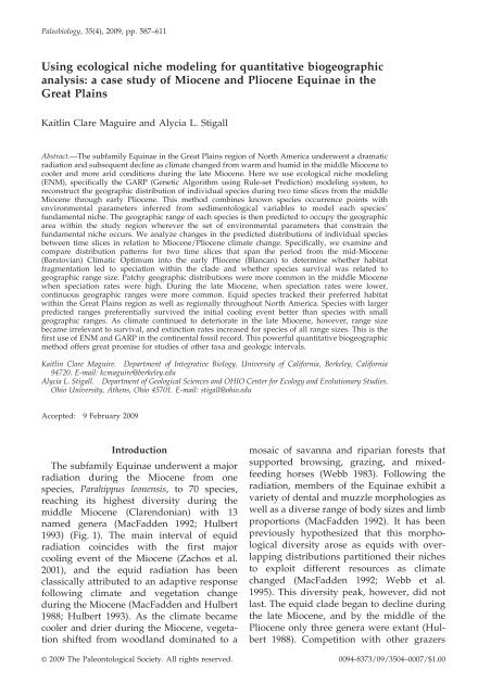
Paleobiology, 35(4), 2009, pp. 587–611 

Using ecological niche modeling for quantitative biogeographic 

analysis: a case study of Miocene and Pliocene Equinae in the 

Great Plains 

Kaitlin Clare Maguire and Alycia L. Stigall 

Abstract.—The subfamily Equinae in the Great Plains region of North America underwent a dramatic 

radiation and subsequent decline as climate changed from warm and humid in the middle Miocene to 

cooler and more arid conditions during the late Miocene. Here we use ecological niche modeling 

(ENM), specifically the GARP (Genetic Algorithm using Rule-set Prediction) modeling system, to 

reconstruct the geographic distribution of individual species during two time slices from the middle 

Miocene through early Pliocene. This method combines known species occurrence points with 

environmental parameters inferred from sedimentological variables to model each species’ 

fundamental niche. The geographic range of each species is then predicted to occupy the geographic 

area within the study region wherever the set of environmental parameters that constrain the 

fundamental niche occurs. We analyze changes in the predicted distributions of individual species 

between time slices in relation to Miocene/Pliocene climate change. Specifically, we examine and 

compare distribution patterns for two time slices that span the period from the mid-Miocene 

(Barstovian) Climatic Optimum into the early Pliocene (Blancan) to determine whether habitat 

fragmentation led to speciation within the clade and whether species survival was related to 

geographic range size. Patchy geographic distributions were more common in the middle Miocene 

when speciation rates were high. During the late Miocene, when speciation rates were lower, 

continuous geographic ranges were more common. Equid species tracked their preferred habitat 

within the Great Plains region as well as regionally throughout North America. Species with larger 

predicted ranges preferentially survived the initial cooling event better than species with small 

geographic ranges. As climate continued to deteriorate in the late Miocene, however, range size 

became irrelevant to survival, and extinction rates increased for species of all range sizes. This is the 

first use of ENM and GARP in the continental fossil record. This powerful quantitative biogeographic 

method offers great promise for studies of other taxa and geologic intervals. 

Kaitlin Clare Maguire. Department of Integrative Biology, University of California, Berkeley, California 

94720. E-mail: kcmaguire@berkeley.edu 

Alycia L. Stigall. Department of Geological Sciences and OHIO Center for Ecology and Evolutionary Studies, 

Ohio University, Athens, Ohio 45701. E-mail: stigall@ohio.edu 

Accepted: 9 February 2009 

Introduction 

The subfamily Equinae underwent a major 

radiation during the Miocene from one 

species, Parahippus leonensis, to 70 species, 

reaching its highest diversity during the 

middle Miocene (Clarendonian) with 13 

named genera (MacFadden 1992; Hulbert 

1993) (Fig. 1). The main interval of equid 

radiation coincides with the first major 

cooling event of the Miocene (Zachos et al. 

2001), and the equid radiation has been 

classically attributed to an adaptive response 

following climate and vegetation change 

during the Miocene (MacFadden and Hulbert 

1988; Hulbert 1993). As the climate became 

cooler and drier during the Miocene, vegetation 

shifted from woodland dominated to a 

mosaic of savanna and riparian forests that 

supported browsing, grazing, and mixedfeeding 

horses (Webb 1983). Following the 

radiation, members of the Equinae exhibit a 

variety of dental and muzzle morphologies as 

well as a diverse range of body sizes and limb 

proportions (MacFadden 1992). It has been 

previously hypothesized that this morphological 

diversity arose as equids with overlapping 

distributions partitioned their niches 

to exploit different resources as climate 

changed (MacFadden 1992; Webb et al. 

1995). This diversity peak, however, did not 

last. The equid clade began to decline during 

the late Miocene, and by the middle of the 

Pliocene only three genera were extant (Hulbert 

1988). Competition with other grazers 

’ 2009 The Paleontological Society. All rights reserved. 0094-8373/09/3504–0007/$1.00

588 KAITLIN C. MAGUIRE AND ALYCIA L. STIGALL 

FIGURE 1. Temporally calibrated cladogram of Equinae modified from Maguire and Stigall (2008). Time slice divisions 

are indicated at the top. Narrow horizontal lines indicate ghost lineages, whereas bold horizontal lines indicate the 

recorded range. Thick gray lines indicate species whose ranges were modeled in this analysis.

(e.g., artiodactyls, rodents) was previously 

inferred to have caused the decline of the 

clade (Simpson 1953; Webb 1969, 1984; Stanley 

1974), but it is now attributed to the 

continuation of cooling temperatures and 

more arid climatic conditions (MacFadden 

1992; Webb et al. 1995). 

Most paleobiogeographic studies of equids 

have focused on large-scale patterns, such as 

migration patterns from North America to the 

Old World (e.g., MacFadden 1992). Other 

paleobiogeographic studies have grouped 

equids with other Miocene mammalian clades 

to demonstrate general patterns, such as 

retreat to the Gulf Coast region as the climate 

became cooler and more arid in northern areas 

of North America during the late Miocene 

(e.g., Webb 1987; Webb et al. 1995). A more 

focused study examining the distribution of 

individual equid species can provide a framework 

in which to analyze habitat fragmentation, 

niche partitioning, and speciation. Because 

the radiation is hypothesized to have 

resulted from climate change, an integrated 

assessment of the ecology and biogeography is 

necessary to fully understand evolutionary 

patterns in the clade. Shotwell (1961) recognized 

this relationship in his study on the 

biogeography of horses in the northern Great 

Basin, in which he observed changes in species 

composition that coincided with vegetation 

change. Shotwell concluded that this shift 

resulted from immigration of equid species 

adapted to the new vegetative regime from 

other regions into the Great Basin. 

Recent advances in understanding the 

phylogenetic relationships provide a more 

robust framework for new analyses. Furthermore, 

numerous recent studies have investigated 

the environmental and climatic conditions 

of the Great Plains during the Miocene. 

These studies comprise analyses of vegetation 

type (e.g., Fox and Koch 2003; Strömberg 

2004; Thomasson 2005), paleosol composition 

(e.g., Retallack 1997, 2007), and climate 

proxies including stable oxygen and carbon 

isotopes of foraminifera from deep-sea cores 

(e.g., Woodruff et al. 1981; Zachos et al. 2001) 

that provide a rich source of environmental 

information previously unavailable for equid 

ecological biogeographic analyses. 

ECOLOGICAL NICHE MODELING OF EQUINAE 589 

Although the diversification of the Equinae 

is hypothesized to have resulted from climate 

change and ecological specialization, the 

interaction between individual species and 

environmental conditions has not previously 

been quantitatively analyzed. Here we reconstruct 

the geographic ranges for individual 

species of Miocene to early Pliocene horses in 

concert with environmental conditions to 

assess how changing climate and shifting 

habitats affected evolutionary patterns in the 

Equinae. In order to study the distribution of 

horses relative to ecological changes, we use 

ecological niche modeling (ENM). A species’ 

ecological, or fundamental, niche is defined as 

the set of environmental tolerances and limits 

in multidimensional space that defines where 

a species is potentially able to maintain 

populations (Grinnell 1917; Hutchinson 

1957). Determining the ecological niche of a 

taxon is essential in determining its potential 

distribution (Peterson 2001) as well as taxon/ 

environment interactions. A species may 

potentially occupy the entire geographic 

region in which its ecological niche occurs; 

although biotic interactions, including competition 

and predation may limit a species 

range to a smaller ‘‘realized niche’’ (Lomolino 

et al. 2006). Because determination of these 

biotic interactions from the fossil record is 

rarely possible, we turn here instead to 

modeling species’ ecological niches. 

Ecological niche modeling is a GIS-based 

method in which species’ environmental 

tolerances are modeled on the basis of a set 

of environmental conditions at locations 

where the species is known to occur. The 

species range is then predicted to occupy 

areas where the same set of environmental 

conditions occurs in the study region. Fundamentally, 

this approach directly utilizes sedimentary 

data to determine the likely distribution 

of taxa, thus providing a framework to 

examine interactions between abiotic and 

biotic factors that control species distribution 

and how these shift through time. ENMbased 

range prediction provides a framework 

to test hypotheses about similarities/differences 

in evolutionary and/or biogeographic 

patterns exhibited as climate and environments 

shifts through time (Stigall and Lieber-


man 2006; Stigall 2008). ENM methods were 

originally developed for modern taxa, and 

high levels of predictive accuracy have been 

documented (Peterson and Cohoon 1999; 

Peterson 2001; Stockwell and Peterson 2002). 

In particular, analyzing niche conservatism 

versus niche shifts in ecological time (e.g., 

Peterson et al. 2001, 2002; Nunes et al. 2007) 

and predicting the extent of species occurrences 

for conservation purposes (e.g., Peterson 

et al. 1999; Raxworthy et al. 2003) have 

been highly productive. The only prior use of 

ENM methods for the fossil record examined 

the geographic ranges of Late Devonian 

brachiopods in the north Appalachian Basin 

across the Frasnian/Famennian (Late Devonian) 

boundary (Stigall Rode and Lieberman 

2005). Results of that study indicated that the 

computer-learning-based algorithms used in 

ENM have excellent potential to predict fossil 

species ranges from sedimentary parameters. 

This study uses the GARP (Genetic Algorithm 

using Rule-set Prediction) modeling system, a 

computer-learning-based analytical ENM 

package (Stockwell and Peters 1999). GARP 

has been successfully used with numerous 

modern mammalian studies investigating 

ecological and environmental questions (e.g., 

Lim et al. 2002; Illoldi-Rangel and Sánchez- 

Cordero 2004) and in studies of marine 

invertebrates in the fossil record (Stigall Rode 

and Lieberman 2005). This study represents 

the first application of ENM and GARP to 

fossil vertebrates. The fossil record of equids 

is densely sampled and abundant locality 

information provides a robust record of 

where each species lived in North America 

(MacFadden 1992). This clade, therefore, is an 

excellent candidate for ENM analysis. Direct 

mapping of species ranges from known 

occurrence points may underestimate a species’ 

actual geographic range because of the 

inherent biases of the paleontological record 

(Kidwell and Flessa 1996; Stigall Rode 2005). 

More accurate ranges can be constructed by 

using ENM to model species ranges on the 

basis of known occurrence points and environmental 

parameters estimated from the 

sedimentary record (Maguire 2008). 

In this study, the distribution patterns of 

individual species are examined to better 

constrain the rise and fall of the Equinae in 

relation to environmental and climatic 

change. We model ecological niches and 

predict geographic ranges in order to study 

how species’ distributions shifted through 

time as a result of climatic and vegetative 

changes. Specifically, we test hypotheses that 

habitat fragmentation led to the diversification 

of the clade and that distributional 

patterns and range size affected the survivorship 

of individual species are tested. 

Methods 

Geographic and Stratigraphic Intervals 

Geographic Extent.—The geographic distributions 

of equid species were reconstructed 

for each of two successive time slices during 

the middle Miocene through early Pliocene in 

the Great Plains region of North America 

(Table 1). The study area incorporated regions 

of the High Plains, as defined by 

Trimble (1980), which comprises northern 

Texas, western Oklahoma, western Kansas, 

Nebraska, eastern Colorado, southeastern 

Wyoming, and southern South Dakota 

(Fig. 2). Although equid species also inhabited 

regions of North America outside the 

study area, we focus our analysis on the 

Great Plains region because there is abundant 

published data on both the distribution of 

equid fossil material and the environmental 

setting of the region during the Miocene and 

Pliocene. To facilitate analysis of environmental 

data, we divided the study region into grid 

boxes of 1u longitude by 1u latitude (Fig. 2). 

Subdivision of geographic regions at this 

scale is standard procedure for ENM analyses 

of modern organisms (e.g., Stockwell and 

Peterson 2002; Wiley et al. 2003; Illoldi-Rangel 

and Sánchez-Cordero 2004), and modern 

environmental data are typically presented 

in this format. Environmental parameter data 

were collected for as many 1u grid boxes as 

possible from literature sources (Tables 2, 3, 4). 

Climatic, Temporal, and Stratigraphic Framework.—Data 

were collected for two time slices 

(Barstovian–Clarendonian and Hemphillian– 

Blancan) in order to analyze the distribution 

of species through the climatic changes of the 

Miocene and Pliocene. Boundaries for each

FIGURE 2. Study area overlain with 1u 3 1u grid boxes illustrating the distribution of environmental data (black circles) 

and species occurrence data (white triangles) for the Barstovian–Clarendonian (A) and Hemphillian–Blancan (B) time 

slices. Base map indicates paleoelevation in meters, modified from Markwick (2007). 

time slice (Table 1, Fig. 1) were based on 

changes in slope or directional reversals of 

temperature trends in the Cenozoic climate 

curve of Zachos et al. (2001). This climate 

curve is a compilation of global deep-sea 

oxygen and carbon isotope records of benthic 

foraminifera from over 40 Deep Sea Drilling 

Project and Ocean Drilling Program sites 

culled from the literature (Zachos et al. 2001) 

and is the Cenozoic climate curve most 


widely used in the literature (e.g., Barnosky 

and Kraatz 2007; Berger 2007; Costeur and 

Legendre 2008; Gamble et al. 2008; Williams 

et al. 2008). 

The first interval examined in this analysis 

spans a 5.5 Ma interval from the middle 

Barstovian North American Land Mammal 

Age (NALMA), as temperatures began to 

drop dramatically following the Mid-Miocene 

Climatic Optimum (ca. 11.5 Ma), through the 

TABLE 1. Species included in niche modeling analysis by time slice. Number in parentheses indicates number of 

spatially distinct species occurrences included in modeling analysis. 

Barstovian–Clarendonian Hemphillian–Blancan 

Calippus martini (25) Astrohippus ansae (9) 

Calippus placidus (24) Astrohippus stockii (7) 

Calippus regulus (17) Cormohipparion occidentale (8) 

Cormohipparion occidentale (44) Dinohippus interpolatus (12) 

Cormohipparion quinni (12) Dinohippus leidyanus (8) 

Hipparion tehonense (11) Equus simplicidens (19) 

Merychippus coloradensis (12) Nannippus aztecus (8) 

Merychippus insignis (15) Nannippus lenticularis (18) 

Merychippus republicanus (18) Nannippus peninsulatus (8) 

Neohipparion affine (30) Neohipparion eurystyle (27) 

Neohipparion trampasense (5) Neohipparion leptode (10) 

Pliohippus mirabilis (11) Pliohippus nobilis (9) 

Pliohippus pernix (28) 

Protohippus perditus (18) 

Protohippus supremus (26) 

Pseudhipparion gratum (37) 

Pseudhipparion hessei (10) 

Pseudhipparion retrusum (24) 

Protohippus gidleyi (5)


TABLE 2. Environmental variables studied and 

primary references. 

1. Percent C4 vegetation (stable isotope data based on 

tooth enamel* or paleosols{) 

Fox and Fisher 2004* 

Fox and Koch 2003{ 

Passey et al. 2002* 

Wang et al. 1994* 

Clouthier 1994* 

2. Mean annual precipitation (MAP) 

Damuth et al. 2002 

Retallack 2007 

Retallack unpublished data 

3. Mollic epipedon 

Retallack 1997 

Retallack unpublished data 

4. Ecotope 

Axelrod 1985 

Gabel et al. 1998 

MacGinitie 1962 

Strömberg 2004 

Thomasson 1980, 1983, 1990, 1991, 2005 

Wheeler and Mayden 1977 

5. Crocodilian distribution 

Markwick 2007 

end of the Clarendonian NALMA. Stable 

oxygen isotope data from benthic foraminifera 

indicate falling temperatures during this 

time that fluctuated with an overall drop from 

13uC to about 7.5–9.5uC (Cooke et al. 2008). 

This interval of global cooling was mediated 

by the formation of permanent ice sheets on 

Antarctica (Woodruff et al. 1981; Zachos et al. 

2001; Rocchi et al. 2006; Lewis et al. 2007). 

Uplift of the Cordilleran region during the 

Miocene resulted in development of a rainshadow 

effect, which in concert with the 

cooling temperatures, resulted in increased 

aridity in the Great Plains during the middle 

Miocene (Zubakov and Borzenkova 1990; 

Ward and Carter 1999). Mean annual precipitation 

fluctuated between 1000 mm and 

500 mm during this period, with an overall 

trend of decreasing precipitation (Retallack 

2007). Streams flowing eastward from the 

Cordillera deposited sediment on the Great 

Plains forming the Ogallala Group, an east- 

TABLE 3. Environmental data for each grid box in the Barstovian–Clarendonian. MAP 5 mean annual precipitation. 

Values in parentheses indicate number of data points within the grid box. Coding for environmental variables as 

follows: Mollic epipedon: 1 5 mollic, 2 5 near-mollic, 3 5 non-mollic. Ecotope: 1 5 woodland, 2 5 savanna with 

surrounding woodland, 3 5 savanna, 4 5 grassland/steppe. Crocodiles: 0 5 absence, 1 5 presence. Decimal values 

represent averaged values where multiple data points occur in a single grid box. 

Long. Lat. % C4 MAP (mm) Mollic epipedon Ecotope Crocodilian presence 

2102.5 43.5 - - - 3 (1) - 

2101.5 43.5 - 266.17 (1) 3 (1) 3 (11) - 

2100.5 43.5 - - - - 0 (1) 

299.5 43.5 - 356.31 (17) 2.9 (17) 3 (9) 0 (1) 

297.5 42.5 13 (1) - - - 1 (2) 

298.5 42.5 16 (3) 1590.65 (1) - 2.5 (2) 1 (1) 

299.5 42.5 18.4 (6) 819.07 (4) 2 (3) 3 (7) 0 (3) 

2100.5 42.5 10.6 (5) 519.57 (15) 2.1 (13) 3 (12) 1 (1) 

2101.5 42.5 15 (1) 825 (1) - 2.8 (4) - 

2102.5 42.5 16 (1) - - - 0 (1) 

2103.5 42.5 13.5 (3) 410.34 (9) 1 (8) - 1 (2) 

2104.5 41.5 - 325.86 (1) - - 0 (1) 

2103.5 41.5 18.5 (2) - - - 0 (1) 

2102.5 41.5 28 (1) 479.59 (3) 2 (2) 2 (1) - 

2101.5 41.5 16 (1) - - - - 

298.5 40.5 0 (1) 1888.09 (1) - - 0 (1) 

2100.5 40.5 23 (1) - - - - 

2103.5 40.5 - 1143.92 (1) - 1 (1) - 

2104.5 40.5 - 633.87 (1) - - - 

2100.5 39.5 21 (1) 402.61 (2) 2.5 (2) 2 (1) - 

299.5 39.5 - 266.53 (1) - - 0 (1) 

299.5 37.5 - - - - - 

299.5 36.5 17.3 (3) - - - - 

2100.5 36.5 18 (1) 825 (1) - - 1 (1) 

2101.5 36.5 12 (1) - - - 1 (1) 

2100.5 35.5 5 (1) - - - 1 (2) 

2100.5 34.5 1 (1) 760 (1) - 3 (1) 0 (1) 

2101.5 33.5 29 (2) - - - -

TABLE 4. Environmental data for each grid box in the Hemphillian–Blancan time slice. Refer to Table 3 for explanation. 

Long. Lat. % C4 MAP (mm) Mollic epipedon Ecotope Crocodilian presence 

298.5 43.5 59 (1) 323.53 (1) - - - 

297.5 42.5 55 (1) 661.38 (2) - - 0 (1) 

298.5 42.5 15 (1) 486.91 (2) - - - 

299.5 42.5 37 (3) 379.16 (5) 1.8 (5) - 0 (1) 

2100.5 42.5 0 (1) 393.11 (1) 2 (1) - - 

2101.5 42.5 58 (1) - - - - 

2103.5 42.5 12 (3) 533.87 (1) - - - 

2103.5 41.5 26 (2) 335.94 (6) 2.2 (6) - - 

2102.5 41.5 27 (5) 349.42 (23) 2.5 (22) 2.7 (3) - 

2101.5 41.5 19 (2) 339.2 (5) 2.3 (4) 2 (1) - 

2100.5 41.5 - 275.54 (1) - - - 

299.5 41.5 15 (1) - - - - 

298.5 41.5 21 (1) - - - - 

297.5 41.5 69 (2) - - - - 

2100.5 40.5 12 (1) 820.2 (1) - - - 

2102.5 40.5 - 520.47 (1) - - - 

2101.5 39.5 - 646.52 (1) - 4 (1) - 

2100.5 39.5 - 429.28 (17) 1.6 (16) - - 

299.5 39.5 - 365.76 (27) 2.3 (27) 2 (2) - 

297.5 39.5 - 181.26 (1) - - - 

299.5 38.5 - 252.52 (2) 3 (2) - - 

2100.5 38.5 - 356.51 (27) 2.9 (27) 2 (1) - 

2100.5 37.5 38 (2) 503.01 (42) 2.5 (41) - 0 (5) 

299.5 37.5 8 (1) 148.43 (1) - - - 

299.5 36.5 4 (1) - - - 0 (2) 

2100.5 36.5 9.5 (2) - - 3 (1) 0 (3) 

2101.5 36.5 - - - - 1 (1) 

2102.5 35.5 - - - - 0 (1) 

2101.5 35.5 37 (2) - - - 0 (3) 

2100.5 35.5 21 (1) - - - 0 (1) 

299.5 34.5 - - - - 0 (1) 

2100.5 34.5 0 (1) - - - - 

2101.5 34.5 43 (3) - - - 0 (2) 

2102.5 34.5 20 (1) - - - 0 (1) 

2102.5 33.5 11 (1) - - - - 

2101.5 33.5 21.5 (2) - - - 1 (3) 

2100.5 33.5 - - - - 0 (1) 

299.5 33.5 - - - - 1 (1) 

ward sloping wedge of coarse fluvial sediments 

that eroded from the Laramie and 

Front Ranges (Condon 2005). The Ogallala 

Group sediments include braided stream, 

alluvial fan, low-relief alluvial plain, and 

lacustrine deposits (Goodwin and Diffendal 

1987; Scott 1982; Swinehart and Diffendal 

1989; Flanagan and Montagne 1993). 

The second time slice comprises 6.5 million 

years and includes the Hemphillian through 

the Blancan North American Land Mammal 

Ages and spans the Miocene-Pliocene boundary. 

Climate fluctuated during this interval, 

but an overall cooling trend continued. 

During the early Hemphillian, temperatures 

stabilized at approximately 8uC but then 

continued to decline, reaching a minimum 

of 4.5uC before rising back to 8uC by the end 


of the Miocene (Zachos et al. 2001; Cooke et 

al. 2008). This cooling was associated with 

increased aridity during the Miocene as mean 

annual precipitation dropped to 250 mm 

(Retallack 2007). During the early Pliocene, 

however, mean annual precipitation increased 

to approximately 1050 mm although 

temperatures continued to cool reaching 

modern temperatures (Chapin and Kelley 

1997; Elias and Mathews 2002). Around 

4 Ma, temperatures rose by 10uC, leading to 

the mid-Pliocene thermal optimum (Elias and 

Mathews 2002). Deposition of the Ogallala 

Group continued during the first half (late 

Miocene portion) of this time slice. Erosion of 

the western mountain ranges slowed during 

the Pliocene, and as deposition slowed, an 

unconformity formed above the Ogallala


Group (Condon 2005). Furthermore, the Great 

Plains region began to slowly uplift (Morrison 

1987). As the region rose, sediments in the 

western Great Plains were eroded and either 

redeposited on top of the Ogallala Group or 

removed completely; however, sediments 

accumulated in Nebraska during the Pliocene 

due to its northeastward slope at the time 

(Steven et al. 1997). 

Species Occurrence Data 

Species occurrence data were collected 

from the primary literature as well as online 

databases (Miocene Mammal Mapping Project 

[MIOMAP]; Carrasco et al. 2005) and the 

Paleobiology Database [PBDB]). Species 

name, geographic occurrence (latitude and 

longitude), and stratigraphic position were 

recorded for each species assigned to the 

subfamily Equinae (see Supplementary Material 

online at http://dx.doi.org/10.1666/ 

08048.s1:). Alroy’s (2002, 2007) reidentifications 

of several specimens in the PBDB 

record were honored. The occurrence data 

were split into the two times slices described 

above. Although species occurrence data 

were collected for all species considered 

valid in recent phylogenetic hypotheses (e.g., 

Hulbert 1993; Kelly 1995, 1998; Prado and 

Alberdi 1996; Woodburne 1996) (Fig. 1), 

species with fewer than five spatially 

distinct occurrences in the study region per 

time slice were excluded from the analysis. 

This cutoff number has been determined from 

modeling experiments to be the minimum 

data required to produce robust ecological 

niche models using the GARP modeling 

system (Peterson and Cohoon 1999; Stockwell 

and Peterson 2002). A recent revision of 

Cormohipparion by Woodburne (2007) was not 

included in this study because that revision 

utilized highly typological species concepts 

that differ from all previous analyses. 

Environmental Data 

A variety of environmental factors (e.g., 

temperature, climate, vegetation, resource 

availability) may determine the ecological 

niche of a horse species. Although biotic 

competition may have played a role in further 

constraining the ranges of certain species, 

particularly species with sympatric ranges 

(e.g., Calippus regulus, C. placidus, and C. 

martini), it is not possible to model these 

interactions within a paleobiologic framework 

or with ENM methods. This analysis, 

therefore, focuses on reconstructing a species’ 

fundamental niche and not its realized niche. 

To model fundamental niches of extinct 

species, environmental factors are estimated 

from sedimentological variables collected 

from the sedimentary record (Stigall Rode 

and Lieberman 2005). This study focused on 

five environmental parameters: percent C 4 

vegetation, mean annual precipitation, soil 

type, ecotope, and crocodilian occurrence (a 

temperature proxy). Each of these parameters 

can be determined from the sedimentary 

record, either through fossils or directly from 

sedimentary deposits. The combination of 

these variables produces a robust data set of 

environmental and climatic factors that can be 

used to reconstruct the distribution of horse 

species. The use of five environmental variables 

is consistent with standard ENM methodology; 

analyses with the GARP modeling 

system have been successful with as few as 

four and as many as 19 environmental factors 

(e.g., Peterson and Cohoon 1999; Anderson et 

al. 2002; Feria and Peterson 2002). Although 

covariation among these environmental variables 

exists (e.g., ecotope and percent C 4 

vegetation), GARP is not sensitive to covariation 

among environmental variables because 

it is a Bayesian-based system that produces 

accurate results for a wide range of domains, 

such as numerical function optimization, 

adaptive control system design, and artificial 

intelligence tasks (Stockwell and Peters 1999). 

Classical and parametric statistics, on the 

other hand, are sensitive to covariation within 

data and, therefore, are not applicable for this 

study. The five environmental parameters are 

discussed individually below, and data are 

presented in Tables 3 and 4. 

Stable Carbon Isotopes.—During the Cenozoic, 

the dominant vegetation type shifted from 

enclosed forests with leafy shrubs and trees 

(C3 plants) to grasslands (C4 plants). This shift 

in vegetation created a mosaic of food sources 

for equid taxa during the Miocene, promoting 

a diverse range of morphological feeding

adaptations in the Equinae clade (MacFadden 

1992; Webb et al. 1995). The distribution of a 

species’ food resource is the primary factor 

determining its ecological niche and geographic 

range (Fox and Fisher 2004; Lomolino 

et al. 2006). Carbon isotope composition (d 13 C) 

can be used as a proxy for vegetation type (C 3 

or C4) in the Great Plains. C3 and C4 plants 

use different photosynthetic pathways (Calvin 

cycle and Hatch-Slack cycle, respectively) 

for fixing atmospheric CO2 (Cerling and 

Quade 1993). Each pathway fractionates 

carbon isotopes to a different degree, producing 

nonoverlapping carbon isotope compositions. 

Modern C 3 plants exhibit a d 13 C range 

of 222% to 235% with an average of 227% 

(O’Leary 1988; Tieszen and Boutton 1989), 

whereas modern C4 plants exhibit a range of 

210% to 214% with an average of 213% 

(O’Leary 1988; Tieszen and Boutton 1989). A 

third pathway, crassulacean acid metabolism 

(CAM), results in carbon isotope compositions 

intermediate to the other two pathways, 

but it is primarily utilized by succulent plants 

in arid conditions (Cerling and Quade 1993) 

and uncommon in the study area. 

Stable carbon isotope data included in this 

study were assembled from published literature 

sources that analyzed d 13 C primarily 

from paleosols (Table 2). Stable carbon isotope 

data from tooth enamel of equids and 

proboscideans were also used to supplement 

the larger paleosol data set (Table 2). The use 

of stable carbon isotope values from tooth 

enamel has been used as a vegetation proxy 

in previous analyses (e.g., Wang et al. 1994; 

Cerling et al. 1997; Passey et al. 2002). While 

we recognize that values from tooth enamel 

may be more indicative of diet type than of 

overall environment in certain taxa, we have 

combined stable carbon isotope data from 

multiple taxa in order to prevent bias in the 

data set. Studies of carbon isotopes in 

paleosols applied an enrichment value of 

+14–17% to all values according to Cerling 

et al. (1989, 1991). Enamel studies applied an 

enrichment factor of +14% to all values 

according to Cerling and Harris (1999). 

Published d 13 C values also control for the 

1.5% decrease in the atmospheric composition 

of CO2 that has occurred since the onset 


of human fossil fuel burning (Friedli et al. 

1986). We used the results of Fox and Koch 

(2003) and Passey et al. (2002) to convert raw 

stable carbon isotope data into percent C4 

vegetation. Percent C 4 vegetation was used as 

an index of the vegetative composition. Low 

C4 percentages are interpreted as predominantly 

leafy vegetation preferred by browsers, 

high percentages are interpreted as 

predominantly grassy vegetation preferred 

by grazers, and intermediate percentages 

represent vegetation preferred by mixed 

feeders. 

Mean Annual Precipitation.—Rainfall would 

have directly influenced the vegetation and 

water resources available to equid species 

and thus represents a fundamental parameter 

of a species’ ecological niche (e.g., Anderson 

et al. 2002; Illoldi-Rangel and Sánchez-Cordero 

2004). Mean annual precipitation (MAP) 

values determined from paleosols, ungulate 

tooth size, and vegetation were compiled for 

analysis (Table 2). The depth of the Bk 

horizon in paleosols can be utilized to 

estimate MAP with the equation: p 5 137.24 

+ 6.45D 2 0.013D 2 , where D is depth in cm 

(Jenny 1941; Retallack 1994, 2005). A second 

measure of MAP, which uses ungulate tooth 

size within a community, is ‘‘per-species 

mean hypsodonty’’ (PMH). Developed by 

Damuth et al. (2002), PMH is the average 

hypsodonty of the ungulate fauna divided by 

the number of all mammalian species present 

in a community (Janis et al. 2004). Lastly, we 

used MAP ranges interpreted from plant 

assemblages (Axelrod 1985; Thomasson 1980). 

Mollic Horizon.—Soil horizons can provide 

information about precipitation, climate, and 

vegetation cover. As discussed above, these 

factors influence the distribution of species. 

Modern soils supporting grassy vegetation 

have a mollic epipedon, a surface layer 

consisting of dark organic clayey soil about 

2–5 mm thick (Retallack 1997). In paleosols, 

mollic epipedons are recognized by common 

dark, thin, clayey rinds to abundant small 

rounded soil peds and by abundant fine root 

traces. In addition, fossilized mollic epipedons 

are nutrient-rich and often contain 

carbonate or easily weathered minerals. Retallack 

(1997, personal communication 2007)


divided paleosols containing calcareous nodules 

from the Great Plains during the Miocene 

into three categories. The first category, mollic, 

contained all paleosols that adhered to the 

above criteria. The second category, nearmollic, 

was assigned to paleosols that had 

surface horizons with ‘‘a structure of subangular 

to rounded peds some 5–10 mm in size, 

along with abundant fine root traces and 

darker color than associated horizons’’ (Retallack 

1997). Near-mollic epipedons are found 

under bunch grasslands of woodlands or 

under desert grasslands (Retallack 1997). The 

third category, non-mollic, was assigned to all 

other paleosols included in the study. This 

third group consisted primarily of paleosols 

similar to soils of deserts and woodlands 

(Retallack 1997). We coded the vegetation 

cover interpreted from the three categories of 

mollic epipedons as 1, 2, and 3, respectively. 

Ecotope.—The fourth environmental variable 

included in this analysis is ecosystem 

type as determined from paleobotanical studies 

(Table 2). Although an extensive collection 

of paleobotanical occurrences and taxonomic 

descriptions exists in the literature, only 

studies that included a paleoenvironmental 

description were included in the data set for 

this analysis. These environmental descriptions 

were coded and divided into four 

categories: 

1. Woodland (e.g., ‘‘deciduous valley and 

riparian forests with scattered grasslands’’ 

[Axelrod 1985]) 

2. Savanna or subtropical grassland with 

surrounding wooded areas (e.g., ‘‘subtropical 

grassland with associated mesic 

and woody components’’ [Thomasson 

2005]) 

3. Savanna or subtropical grassland (e.g., 

‘‘grassland savanna’’ [Gabel et al. 1998]) 

4. Dominantly grassland/Steppe (e.g., 

‘‘grassland, shrubs, with limited trees’’ 

[Thomasson 1990]) 

Crocodilian Distribution.—In the fossil record, 

crocodilian occurrence has traditionally 

been used as a paleotemperature proxy (Lyell 

1830; Owen 1850). Ecological analysis of 

modern crocodilians indicates that temperature 

is the most influential factor determining 

their distribution (Woodburne 1959; Martin 

1984; Markwick 1996). The data set used in this 

analysis is derived from the comprehensive 

work of Markwick (1996, 2007). Markwick 

(1996) compiled a global database of vertebrate 

assemblages and used the distribution of 

crocodilians as a paleotemperature proxy from 

the Cretaceous through the Neogene. Markwick 

(1996) includes crocodilians that belong to 

the ‘‘crown group’’ (Alligatoridae, Crocodylidae, 

and Gavialidae families). The climatic 

tolerance of the modern American alligator, 

Alligator mississippiensis, was used as the 

minimum temperature tolerance of extinct 

crocodilians. Alligator mississippiensis can tolerate 

a mean temperature range of 25–35uC. 

Because crocodilians are well documented in 

the fossil record and Markwick (1996, 2007) 

includes vertebrate sites lacking crocodilians as 

a control group, crocodilian absences in his 

database are considered true absences. This 

study includes 95 assemblages from Markwick 

(2007) that fall within the study area. For this 

study, crocodilian presence and absences were 

coded 1 and 0, respectively. 

Creation of Environmental Layers 

For analysis of environmental data, the 

study region was divided into 1u grid boxes 

using latitude and longitude coordinates, as 

discussed above, and environmental parameters 

derived from the literature were assigned 

to the appropriate grid box. When 

multiple data points occurred in one grid box, 

the values were averaged to account for 

environmental variability. This method of 

intermediate coding has been successful with 

ENM analysis and is an effective method of 

representing environmental variability (Stigall 

Rode and Lieberman 2005). Raw data are 

included in the supplementary material. 

Environmental data points for both time 

slices were imported into ArcGIS 9.2 (ESRI 

Inc. 2006). For each environmental variable 

we used four data points to create an 

interpolated surface using inverse distance 

weighting, a method that allows us to use a 

set of scattered points to assign values to 

unknown points. Each interpolated surface 

had a power of 3 (exponent of distance) and

an output cell size of 0.1u (8 3 11 km). 

Interpolation was based on four data points 

because this was the largest number of data 

points appropriate for interpolation that were 

available from all environmental data sets. The 

interpolated environmental area for the Barstovian–Clarendonian 

and the Hemphillian– 

Blancan time slices covered from 104uW,44uNto 

98uW,34uNandfrom104uW,44uNto97uW,33uN, 

respectively. Examples of interpolated environmentalcoveragesareshowninFigure3. 

Distribution Modeling 

A genetic algorithm approach was chosen 

to model the distribution of Equinae species. 

Genetic algorithms have been successfully 


FIGURE 3. Examples of environmental variable interpolations. A, Interpolation of the percentage of C 4 vegetation 

derived from stable isotope data in the Hemphillian–Blancan time slice. B, Interpolation of crocodilian presence/ 

absence data for Barstovian–Clarendonian; 0 5 absence, 1 5 presence. See Figure 2 for base map explanation. 

used in previous niche modeling analyses of 

paleontological data (Stigall Rode and Lieberman 

2005) because genetic algorithms are 

effective for data sets with unequal sampling 

and poorly structured domains (Stockwell 

and Peterson 2002). Other statistical methods 

such as multiple regression and logistic 

regression, assume multivariate normality 

and true absence data. Because absence in 

paleontological data does not necessarily 

represent true absence and multivariate normality 

is unlikely with paleontological data, 

these methods are not suitable here. Genetic 

algorithms apply a series of rules in an 

iterative, evolving manner to the data set 

until maximum significance is reached (Stock-


well and Peters 1999). GARP was specifically 

designed to predict a species’ range from its 

fundamental niche as estimated from environmental 

variables (Peterson and Vieglais 

2001). Another advantage of the GARP 

modeling system is that it was originally 

designed to accommodate for data from 

museum collections; in particular, GARP is 

able to analyze non-uniformly distributed, 

sparse, or patchy data (Peterson and Cohoon 

1999; Stockwell and Peters 1999). Furthermore, 

covariance between environmental variables 

does not negatively affect the model’s 

results (Stockwell and Peters 1999). 

All species distribution modeling was 

performed using DesktopGARP 1.1.4 (www. 

nhm.ku.edu/desktopgarp). GARP is composed 

of eight programs that include data 

preparation, model development, model 

application, and model communication 

(Stockwell and Peters 1999). The GARP 

system divides the data in half to create two 

groups, the test group and the training group. 

A rule (e.g., logit, envelope) is randomly 

selected and applied to the training set. The 

accuracy of the rule is assessed by using 

1250 points from the test data set and 

1250 points randomly resampled from the 

area as a whole. The rule is then modified 

(mutated) and tested again. If accuracy 

increases, the modified rule is incorporated 

into the model; if not, it is excluded. GARP 

creates separate rule sets for each region 

within the study area, rather than forcing a 

global rule across the data. The resulting 

models are more accurate and precise than 

those using global rule methods (Stockwell 

and Peters 1999; Stockwell and Peterson 

2002). The algorithm continues until further 

modification of the rules no longer results in 

improved accuracy or the maximum number 

of iterations set by the operator is reached 

(Stockwell and Noble 1992; Stockwell and 

Peters 1999). 

Prior to performing the modeling analysis, 

the statistical significance of each environmental 

variable was tested using a jackknifing 

procedure. This was accomplished by selecting 

all combinations of rules and selected 

layers for the GARP analysis following Stigall 

Rode and Lieberman (2005). The five most 

abundant species from the Barstovian–Clarendonian 

time slice (Cormohipparion occidentale, 

Neohipparion affine, Pliohippus pernix, 

Protohippus supremus, Pseudhipparion gratum) 

were used in the jackknifing procedure. The 

contribution of each environmental variable 

to model error, measured by omission and 

commission, was analyzed using a multiple 

linear regression analysis in Minitab 14 

(Minitab Inc. 2003). An environmental variable 

was inferred to increase error in the 

model if it was significantly correlated with 

either omission or commission. A multiple 

linear regression analysis was conducted for 

the five species in the Barstovian–Clarendonian 

time slice together as well as each 

individual species in the Barstovian–Clarendonian 

time slice. Although each environmental 

variable is significantly correlated 

with error with at least one species; no 

environmental variable contributed significant 

error in all species. All variables were 

therefore considered valid as environmental 

predictors and were included in the niche 

modeling analysis. 

Niche modeling was performed individually 

for each species in each time slice. All 

rules and all environmental layers to be used 

were selected, and 500 replicate models were 

run for each species with the convergence 

interval set at 0.01. Training points were set to 

50% as discussed above. The best subset 

selection was utilized so that the ten best 

models were chosen, with an omission threshold 

of 10% and a commission threshold of 50%. 

Range predictions were output as ASCII grids 

and the ten best models were imported into 

ArcGIS 9.2. The ASCII grids were converted 

into raster files and weight-summed to derive 

the final range prediction maps (Fig. 4). The 

geographic area occupied by each species was 

quantified for biogeographic analysis by using 

the Zonal Geometry Tool in the Spatial Analyst 

Toolbox of ArcGIS and then converting the 

number of rasters occupied into percent area 

occupied in km 2 (Table 5). 

Examination of Distributional Patterns and 

Habitat Tracking 

Habitat Fragmentation.—We analyzed the 

relative prevalence of patchy ranges, ranges


FIGURE 4. GARP predicted species distribution maps for Pseudhipparion gratum in the Barstovian–Clarendonian time 

slice (A), Nannippus lenticularis in the Hemphillian–Blancan time slice (B), N. azetecus in the Hemphillian–Blancan time 

slice (C), Astrohippus ansae in the Hemphillian–Blancan time slice (D), Dinohippus interpolatus in the Hemphillian– 

Blancan time slice (E), Pliohippus mirabilis in the Barstovian–Clarendonian time slice (F), P. pernix in the Barstovian– 

Clarendonian time slice (G), and P. nobilis in the Hemphillian–Blancan time slice (H). Color ramp indicates number of 

the ten best models predicting species occurrence.


TABLE 5. Geographic ranges predicted for species in the Barstovian–Clarendonian and Hemphillian–Blancan time 

slices from GARP modeling. Explanation of column headings and abbreviations: Area (km 2 ), total area of predicted 

species range. Coverage, percentage of the study region that is occupied by the predicted species range. Survivor, 

species survival. S, species survived the NALMA boundary. E, species went extinct by the NALMA boundary. 

Southern coverage, percentage of area below 39uN (Hemphillian–Blancan time slice) or 38.5uN (Barstovian– 

Clarendonian time slice) in the study region that is occupied by the predicted species range. No. of populations, the 

number of distinct populations within a predicted species range. NALMA boundary abbreviations: Bar, Barstovian; 

Clar, Clarendonian; Hemph, Hemphillian; Bla, Blancan. 

Species 

Area 

(km 2 ) 

Coverage 

(%) 

Survivor 

Bar/Clar 

in which a species’ distribution includes 

multiple discrete areas of occurrence, versus 

widespread continuous ranges. Habitat fragmentation 

has been hypothesized to contribute 

to the radiation of numerous clades (e.g., 

birds [Mayr 1942]; fishes [Wiley and Mayden 

1985]; mammals [Vrba 1992]). If geographic 

patchiness did promote speciation in equids, 

species should exhibit a higher frequency of 

discrete patches in their predicted ranges 

during the Barstovian–Clarendonian time 

slice when speciation rates were higher 

(Hulbert 1993), than species in the Hemphillian–Blancan 

time slice, when the clade was in 

decline. For each species in each time slice, we 

counted the number of discrete populations 

or patches occupied (Table 5). The extent of a 

Survivor 

Clar/Hemph 

Southern 

coverage (%) 

No. of 

populations Time slice 

Cormohipparion occidentale 2.29 3 10 5 37.45 S S 36.97 2 Bar–Clar 

Calippus martini 2.32 3 10 5 37.88 S E 44.83 2 Bar–Clar 

Calippus placidus 2.64 3 10 5 43.07 S E 50.07 3 Bar–Clar 

Calippus regulus 9.15 3 10 4 14.93 S E 7.13 4 Bar–Clar 

Cormohipparion quinni 6.45 3 10 4 10.53 E - 0.17 2 Bar–Clar 

Hipparion tehonense 1.17 3 10 5 27.93 S S 36.93 3 Bar–Clar 

Merychippus coloradensis 6.76 3 10 4 11.03 E - 0.00 3 Bar–Clar 

Merychippus insignis 1.10 3 10 5 17.95 E - 1.33 3 Bar–Clar 

Merychippus republicanus 8.40 3 10 4 12.70 E - 0.00 2 Bar–Clar 

Neohipparion affine 1.67 3 10 5 27.25 S E 12.93 3 Bar–Clar 

Neohipparion trampasense 9.34 3 10 4 15.25 S S 19.20 2 Bar–Clar 

Pliohippus mirabilis 1.49 3 10 5 24.28 E - 3.57 2 Bar–Clar 

Pliohippus pernix 2.66 3 10 5 43.35 S E 54.20 2 Bar–Clar 

Protohippus perditus 1.52 3 10 5 24.76 E - 6.10 2 Bar–Clar 

Protohippus supremus 1.31 3 10 5 21.30 S E 14.43 2 Bar–Clar 

Pseudhipparion gratum 2.23 3 10 5 36.42 - E 37.23 2 Bar–Clar 

Pseudhipparion hessei 2.05 3 10 5 33.40 - E 49.10 1 Bar–Clar 

Pseudhipparion retrusum 6.83 3 10 4 11.13 E - 0.00 3 Bar–Clar 

Astrohippus ansae 2.35 3 10 5 29.33 - S 31.27 1 Hemph–Bla 

Astrohippus stockii 2.11 3 10 5 26.40 - S 46.83 1 Hemph–Bla 

Cormohipparion occidentale 2.58 3 10 5 32.21 - S 36.47 1 Hemph–Bla 

Dinohippus interpolatus 2.65 3 10 5 33.13 - S 33.79 1 Hemph–Bla 

Dinohippus leidyanus 3.11 3 10 5 38.87 - S 22.52 1 Hemph–Bla 

Equus simplicidens 2.82 3 10 5 35.30 - - 52.00 3 Hemph–Bla 

Nannippus aztecus 1.19 3 10 5 23.87 - - 39.25 1 Hemph–Bla 

Nannippus lenticularis 4.34 3 10 5 54.13 - - 33.04 1 Hemph–Bla 

Nannippus peninsulatus 2.00 3 10 5 24.96 - - 39.25 1 Hemph–Bla 

Neohipparion eurystyle 4.29 3 10 5 53.53 - - 30.42 2 Hemph–Bla 

Neohipparion leptode 3.67 3 10 5 45.80 - - 36.62 2 Hemph–Bla 

Pliohippus nobilis 2.24 3 10 5 28.00 - S 33.45 1 Hemph–Bla 

Protohippus gidleyi 2.64 3 10 5 32.91 - S 29.12 1 Hemph–Bla 

population or patch was defined by a 

contained area that did not have a geographic 

connection with a second population. The 

number of populations per species for each 

time slice was statistically analyzed using a 

two-sample t-test (Table 6). 

Range Shift and Habitat Tracking.—Initial 

examination of range models indicated an 

apparent southward shift of species between 

the time slices, which we analyzed statistically. 

The study area for each species was 

divided in half along the 39uN latitudinal in 

the Barstovian–Clarendonian time slice time 

slice and the 38.5uN latitudinal in the Hemphillian–Blancan 

time slice. For both time 

slices, the percent area occupied by each 

species was calculated using ArcGIS (Ta-

TABLE 6. Two-sample t-test comparing number of discrete populations per time slice. 

Source Sample size (n) Mean Standard deviation SE mean 

Barstovian–Clarendonian 18 2.389 0.698 0.16 

Hemphillian–Blancan 

t statistic 524.50. 

p 5 1.154 3 10 

13 1.308 0.630 0.17 

24 . 

d.f. 5 24. 

ble 5). A two-sample t-test was applied to 

determine whether species in the Hemphillian–Blancan 

time slice occupied a statistically 

larger portion of the southern region of the 

Great Plains than species of the Barstovian– 

Clarendonian time slice, indicating a range 

shift to the south (Table 7). 

Only one species, Cormohipparion occidentale, 

was extant in both time slices. To determine 

whether the shifting distribution of C. occidentale 

from one time slice to another was a 

function of habitat tracking, the niche model 

for the Barstovian–Clarendonian time slice 

was projected onto the Hemphillian–Blancan 

time slice environmental layers (Peterson et al. 

2001) (Fig. 5). If the resulting distributional 

pattern matches the original predicted distribution 

of C. occidentale for the Hemphillian– 

Blancan time slice, then C. occidentale tracked 

its preferred habitat from the Barstovian– 

Clarendonian time slice to the Hemphillian– 

Blancan time slice (i.e., niche conservatism). If 

the distributional patterns do not have a high 

degree of overlap, C. occidentale did not occupy 

the same niche in both time slices, and the 

species would be interpreted to have altered its 

fundamental niche through time (i.e., niche 

evolution). To determine whether the distributions 

were equivalent, the area of overlap 

and areal extent not shared were measured in 

ArcGIS and compared as a percentage of the 

total study area. 

Examination of Species Survival versus 

Range Size.—Whether a general relationship 


between species longevity and predicted 

distribution area occurs was also assessed 

through regression analysis (Table 8). Specifically, 

we tested the hypothesis that species 

with larger range sizes live longer. The 

longevity of each species was determined 

from the literature as illustrated in the 

stratocladogram in Figure 1. We also examined 

the relationship between species survival 

across NALMA divisions and the geographic 

extent of a species’ distributional range. 

Statistical analyses were performed for each 

Land Mammal Age division within the 

temporal extent of this study (Barstovian/ 

Clarendonian, Clarendonian/Hemphillian, and 

Hemphillian/Blancan boundaries). Survival 

across the boundary was compared with the 

size of the species’ predicted range. The area 

of each species range was determined within 

ArcGIS by calculating the sum of the areas in 

which seven or more of the ten best models 

predict occurrence (Table 5). Previous methods 

have summed three of the five best (Lim 

et al. 2002), six of the ten best (e.g., Stigall 

Rode and Lieberman 2005), or all of the ten 

best (Peterson et al. 2002; Nunes et al. 2007), 

so our approach is more conservative. Raw 

area counts were converted into percentage of 

total model areas for the time slice because the 

extent of the niche modeling area differs 

slightly between time slices (Table 5). A 

nonparametric statistical method, Kruskal- 

Wallis, was used to analyze the relationship 

between survival and area because the data 

TABLE 7. Two-sample t-test comparing the area of a species’ geographic range in the Southern Great Plains per 

time slice. 

Source Sample size (n) Mean Standard deviation SE mean 

Barstovian–Clarendonian 18 20.80 20.40 4.8 

Hemphillian–Blancan 

t statistic 522.84. 

p 5 0.009. 

d.f. 5 23. 

13 35.69 7.62 2.1


FIGURE 5. GARP predicted distribution maps. A, Cormohipparion occidentale Barstovian–Clarendonian model projected 

onto the Barstovian–Clarendonian environmental layers. B, C. occidentale range when the Barstovian–Clarendonian 

model is projected onto the Hemphillian–Blancan environmental layers. C, C. occidentale Hemphillian–Blancan model 

projected onto the Hemphillian–Blancan environmental layers. D, C. occidentale range when the Hemphillian–Blancan 

model is projected onto the Barstovian–Clarendonian environment. 

are not normally distributed even after log, 

square root, and arcsine transformations were 

applied (Tables 9, 10). 

Results and Discussion 

Geographic ranges were modeled for 18 

equid species from the Barstovian–Clarendonian 

time slice and 13 species from the 

Hemphillian–Blancan time slice (Table 1, 

Fig. 4). All modeled ranges are included in 

the online Supplementary Material. 

Habitat Fragmentation 

During the Barstovian–Clarendonian time 

slice, species ranges were divided into more 

discrete populations or patches than during 

the Hemphillian–Blancan time slice (twosample 

t-test, p 5 1.15 3 1024 ) (Table 6, cf.

TABLE 8. Linear regression analysis of species longevity 

versus the area of a species’ geographic range. 

Predictor Coefficient SE coefficient t p 

Constant 2.84 0.81 3.51 0.001 

Area 0.01 0.03 0.43 0.670 

Longevity 5 2.84 + 0.01(Area). 

SD 5 1.66. 

R2 5 0.6. 

Fig. 4A,F vs. 4B,E). The relative abundance of 

patchy habitats in the Barstovian–Clarendonian 

time slice correlates with the mid- 

Miocene interval of rapid cooling. Rapid 

cooling has been shown to promote local 

response of the plant communities resulting 

in fragmentation of the previously widespread 

woodlands into isolated patches (Vrba 

1992). Speciation was high during the Barstovian–Clarendonian 

time slice and the 

Equinae reached its highest diversity at this 

time (MacFadden 1992; Hulbert 1993). Fragmentation 

of habitats would necessarily have 

resulted in patchy species distributions. This 

in turn would have promoted niche partitioning 

and speciation via vicariance, giving 

rise to the diverse group of mixed feeders, 

browsers, and grazers that inhabited the 

mosaic of vegetation in the Great Plains 

(Webb et al. 1995). 

Environmental coverages of the Barstovian–Clarendonian 

time slice indicate an area 

of low precipitation, high percentage of C 4 

plants, and an absence of crocodilians that 

spans the central part of the Great Plains 

(Fig. 3B). In several predicted ranges for the 

Barstovian–Clarendonian time slice, this area 

is unoccupied (e.g., Fig. 4A). The environmental 

coverages for the Hemphillian–Blancan 

time slice indicate a return to wetter 

conditions in this area and a more uniform 

environmental distribution throughout the 

TABLE 9. Kruskal-Wallis test comparing the area of 

species’ geographic range versus species survival across 

the Barstovian/Clarendonian boundary. 

Source 

Sample 

size (n) Median 

Average 

rank Z value 

Survive 9 27.93 11.1 2.49 

Extinct 7 13.70 5.1 22.49 

H 5 6.19. 

p 5 0.013. 

d.f. 5 1. 


TABLE 10. Kruskal-Wallis test comparing the area of 

species’ geographic range versus species survival across 

the Clarendonian/Hemphillian boundary. 

Source 

Sample size 

(n) Median 

Average 

rank Z Value 

Survive 9 33.40 10.0 0.40 

Extinct 9 32.21 9.0 20.40 

H 5 0.16. 

p 5 0.691. 

d.f. 5 1. 

study area. Chapin and Kelley (1997) reported 

increased precipitation in the Pliocene based 

on the establishment of drainage systems, the 

erosion of Mesozoic and Cenozoic sediments, 

the opening of previously closed basins, and 

stable isotope compositions of paleosol carbonates 

in arid lands. Modeled species ranges 

for the Hemphillian–Blancan time slice predict 

species occurrence in the central area 

resulting in more continuous ranges from the 

northern to southern part of the study area 

(Fig. 4B). 

Increased continuity of species ranges of 

the Hemphillian–Blancan time slice may 

result partly from the spreading of grasslands 

ca. 6–7 Ma into wetter climatic regions (Retallack 

1997). As grasslands spread throughout 

the Great Plains in the late Miocene and 

Pliocene, habitats became more homogeneous 

(Axelrod 1985; Webb et al. 1995). The available 

range for species adapted to open 

grassland and steppe habitats increased, 

promoting large continuous geographic distributions. 

Continuous ranges resulting from 

lack of geographic barriers between populations 

may have contributed to the reduced 

speciation rates observed within the clade 

(Hulbert 1993) by eliminating opportunities 

for geographic isolation by vicariance, a 

pattern previously observed in Late Devonian 

marine taxa (Stigall 2009). 

Whereas the diversification of the Equinae 

has been attributed to habitat fragmentation 

and niche partitioning (MacFadden 1992), its 

decline has been attributed to the inability of 

species to adapt to climatic deteriorations 

during the late Miocene and Pliocene (Webb 

1983; MacFadden 1992). In Hulbert’s (1993) 

analysis of biodiversity overturn in Miocene 

to Pliocene Equinae, the observed high 

extinction rates in the late Miocene were


coupled with low speciation rates that eventually 

decline to zero. Although climatic 

deterioration, as hypothesized by MacFadden 

(1992), may explain the increased rate of 

extinction, the increase in continuous habitat 

following the spread of grasslands, and the 

concomitant reduction in opportunities for 

speciation, likely contributed significantly to 

the observed reduction in speciation. Maguire 

and Stigall (2008) previously noted that 

speciation by vicariance occurred much less 

frequently in equids than in modern continental 

taxa (e.g., Wiley and Mayden 1985). 

Consequently, this additional reduction in the 

amount of vicariant speciation in the Equinae 

due to geographic continuity during the late 

Miocene and early Pliocene may have been 

influential in the decline of the clade. 

Habitat Tracking 

As temperatures decreased during the 

Miocene and the climate became more arid, 

several species adapted to woodlands and 

savannas rather than open grasslands retreated 

to warmer and wetter regions of North 

America, specifically the southern Great 

Plains and Gulf Coast regions (e.g., Nannippus 

aztecus, Fig. 4C) (Webb et al. 1995). Using data 

from carbonate nodules, Retallack (2007) 

identified a climatic gradient from warm 

and humid in the coastal regions to cool and 

arid in the northern Great Plains region. 

Species of Equinae in the Hemphillian–Blancan 

time slice of this study occupied larger 

ranges south of 38.5uN, than species of the 

Barstovian–Clarendonian time slice below 

39uN (two-sample t-test, p 5 0.009) (Table 7). 

This southward biogeographic shift indicates 

that species tracked their preferred habitat 

toward the south as climate changed more 

drastically in the northern regions of North 

America. This demonstrates the potential use 

of ENM and the fossil record as tools to track 

patterns of climate change and biogeographical 

responses. Further examination of morphological 

differences and dietary adaptations 

between species that migrated south 

and those that retained a northern range 

would further test this hypothesis. The 

southward range shift may partially result 

from the distribution of species occurrence 

points (Fig. 2). The early time slice has a 

higher concentration of species occurrence 

points in the northern part of the Great Plains, 

whereas the late time slice has a more even 

distribution of points across the Great Plains. 

Because the GARP algorithm is designed to 

analyze data from poorly structured domains 

including unevenly distributed species occurrence 

data (Stockwell and Peterson 2002), the 

uneven data distribution is unlikely to skew 

the resulting range predictions significantly. 

Furthermore, the distribution of occurrence 

points in the early time slice may in fact be an 

accurate representation of the distribution of 

Equinae species, and thus the more northern 

range of equids relative to the late time slice. 

By the Hemphillian, the southwestern 

region of North America was semiarid and 

dominated by shrubland vegetation (Axelrod 

1985). Many ungulates retreated from this 

region into the Great Plains (Webb et al. 1995). 

This included five species that were modeled 

in the Hemphillian–Blancan time slice: Dinohippus 

leidyanus, Dinohippus interpolatus, Equus 

simplicidens, Astrohippus ansae, and Astrohippus 

stockii (Maguire and Stigall 2008). Maguire 

and Stigall (2008) determined that speciation 

of these five taxa was a result of geodispersal 

across the Rocky Mountains from the Southwest 

to the Great Plains. Predicted geographic 

distributions of these five species are similar 

and occur predominantly on the western edge 

of the Great Plains region (Fig. 4D,E). During 

the Neogene, the uplift of the Rocky Mountains 

was interrupted by intervals of tectonic 

quiescence (Condon 2005). Consequently, 

during these intervals of quiescence and 

erosion, equid species could migrate across 

the Cordilleran region, whereas orogenic 

pulses resulted in barriers to species movement. 

The distribution patterns predicted 

from niche modeling supports the conclusion 

of Maguire and Stigall (2008) that speciation 

of these five species was a result of a cyclical 

geodispersal process as habitat tracking occurred 

across the Rocky Mountains during 

these tectonic cycles. 

As mentioned previously, one species, 

Cormohipparion occidentale, was extant during 

both time slices. The species’ predicted 

distributions for the Barstovian–Clarendonian

and Hemphillian–Blancan time slices are 

illustrated in Figure 5A and 5C, respectively. 

Any ecological niche model, for example the 

Barstovian–Clarendonian time slice model, is 

based on the relationship between a species 

and its inferred habitat. Once the ecological 

niche of a species is quantified through 

GARP, it is possible to project the model of 

species occurrence onto either the set of 

environmental variables for the same time 

slice (which was conducted for all taxa in the 

data set) or a different time slice. To test for 

patterns of habitat tracking, the ecological 

niche model of C. occidentale developed from 

the Barstovian–Clarendonian time slice was 

projected onto the environmental layers of 

both the Barstovian–Clarendonian and Hemphillian–Blancan 

time slices, as illustrated in 

Figure 5A and 5B, respectively. Similarly, the 

ecological niche model developed from the 

Hemphillian–Blancan time slice environmental 

data for C. occidentale was projected onto 

both the Barstovian–Clarendonian and Hemphillian–Blancan 

time slices, as illustrated in 

Figure 5C and 5D, respectively. The percentage 

of overlap of the original projection and 

the new prediction in the second time slice 

indicates the extent to which the relationship 

between the species and its preferred habitat 

held constant between both time slices. The 

consistency of this relationship can be referred 

to as habitat tracking. 

Projection of the GARP model for the 

Barstovian–Clarendonian time slice onto the 

environmental layers of the Hemphillian– 

Blancan time slice produced a distribution 

that covered 49% of the area originally 

predicted for the Hemphillian–Blancan time 

slice (Fig. 5B,C). This percentage of overlap 

suggests that Cormohipparion occidentale 

tracked its preferred habitat from the Barstovian–Clarendonian 

time slice into the Hemphillian–Blancan 

time slice. In addition, projection 

of the Hemphillian–Blancan time slice 

GARP model onto the Barstovian–Clarendonian 

time slice environmental layers produced 

a distribution that was 52% similar to 

the original distribution for the Barstovian– 

Clarendonian time slice (Fig. 5A,D). The 

predicted distribution maps show that during 

the Barstovian–Clarendonian time slice, the 


species’ niche does not occupy the central 

region of the study area (Fig. 5A). In the 

Hemphillian–Blancan time slice, however, the 

predicted range does cover this central area, 

indicating that C. occidentale spread through 

this region as it tracked its habitat (Fig. 5D). 

Unlike other genera of Equinae, Cormohipparion 

migrated to the Old World during the 

Miocene (Skinner and MacFadden 1977; Mac- 

Fadden 1992) possibly along with the genus 

Hipparion (but see Bernor and Armour-Chelu 

1999). Cormohippairon was also one of the last 

genera remaining in North America at the 

end of the Miocene (C. emsliei survived in the 

coastal regions through the Blancan). The 

combination of its longevity and large range 

may be a result of its ability to track its 

preferred habitat when climate shifted. 

Range Size versus Survival 

A positive relationship between geographic 

range size and species longevity has been 

documented in many clades (Stanley 1979; 

Vrba 1987; Rode and Lieberman 2004; Hendricks 

et al. 2008). This relationship has not 

been quantitatively assessed in prior analyses 

of equid biogeography; however, this relationship 

can be analyzed statistically with the 

niche models constructed in this study. No 

significant relationship between predicted 

range size and longevity was recovered when 

all species ranges modeled from both time 

slices were combined in a single regression 

analysis (p 5 0.670; Table 8). However, when 

the size of a species’ geographic range was 

compared with survival or extinction across 

specific boundaries between NALMA divisions, 

a significant relationship emerged. The 

NALMA divisions (Alroy 2003) are based on 

first and last appearance data of all mammals 

in North America and are neither dependent 

on ‘‘immigrant first appearance datum’’ nor 

heavily dependent on geochronology data. 

Species living in the Barstovian that survived 

into the Clarendonian had statistically larger 

ranges than species that became extinct by the 

end of the Barstovian (Kruskal-Wallis test, p 

5 0.013; Table 9). Clarendonian species that 

survived into the Hemphillian did not have 

significantly larger ranges than species that 

became extinct (Kruskal-Wallis test, p 5 0.691;


Table 10). Because only one species of Equinae 

modeled in this study had a stratigraphic 

range through the Miocene/Pliocene boundary, 

analysis of range size and survival from 

the Hemphillian to the Blancan was not 

possible. 

The relationship between survival from one 

NALMA to another and species range size is 

likely related to changes in climate and 

vegetation during these intervals. During the 

Barstovian, temperatures dropped quickly 

from 13uC to 7.5–9.5uC (Zachos et al. 2001; 

Cooke et al. 2008). During this interval of 

climate change, vegetation cover was shifting 

and patchy. Under those conditions, the range 

size of individual species was related to 

survival into the Clarendonian. Range size is 

a function of ecological tolerance; consequently 

species with larger ranges were potentially 

more broadly adapted and better able to 

persist through the changing environmental 

conditions. The rapidly changing conditions, 

however, likely were too severe for those with 

smaller ranges and more restricted ecological 

tolerances to survive. During the late Miocene, 

however, species range size was irrelevant 

to survival. Temperatures continued to 

drop to approximately 2.3uC during the 

Clarendonian and Hemphillian, accompanied 

by decreasing MAP that reached 500 mm 

(Zachos et al. 2001; Retallack 2007; Cooke et 

al. 2008). Climatic deterioration became too 

severe even for those species with large 

ranges and broad ecological tolerances to 

survive. 

Regional Trends 

Although the Great Plains is analyzed as a 

case study for niche modeling because of its 

wealth of available data, equid species also 

inhabited other regions of North America 

during the Miocene. Dispersal between the 

Great Plains and other regions was frequent, 

and the resulting distribution patterns influenced 

speciation patterns within the clade 

(Maguire and Stigall 2008). One particular 

genus, Pliohippus, clearly demonstrates the 

relationship between regional patterns and 

local (ecological) patterns in the Great Plains 

region. 

Pliohippus mirabilis occupied a patchy distribution 

in the Great Plains during the 

Barstovian–Clarendonian time slice (Fig. 4F) 

that covered 24.3% of the study area. Pliohippus 

pernix has been hypothesized to have 

evolved from P. mirabilis via anagenetic 

speciation (Hulbert 1993). The patchy pattern 

of P. mirabilis supports the interpretation that 

vicariance following habitat fragmentation 

could have led to the speciation of P. pernix 

from an isolated population of P. mirabilis. 

During the Barstovian–Clarendonian time 

slice, Pliohippus pernix occupied a continuous 

range throughout the Great Plains that covered 

43.4% of the study area (Fig. 4G). This 

range is larger and more continuous than 

other ranges modeled for middle Miocene 

equid species and suggests that P. pernix may 

have been an ecological generalist. In fact, P. 

pernix dispersed into the Gulf Coast in the 

Barstovian–Clarendonian time slice, which 

further supports a generalist interpretation 

(Maguire and Stigall 2008). The populations 

of P. pernix that remained in the Great Plains 

are hypothesized to have evolved anagenetically 

into P. nobilis (Hulbert 1993). Pliohippus 

nobilis occupied a patchy predicted distribution 

in the Great Plains that covered 28% of 

the total area (Fig. 4H). Although P. nobilis 

occupied a predominantly southern distribution 

in the Great Plains, this species remained 

in the Great Plains during the late Miocene 

and did not disperse to other regions of North 

America. The patchy geographic range of P. 

nobilis indicates the limited extent of suitable 

habitat for the species in the Great Plains, 

potentially an ecological specialist. This ecological 

restriction may have prevented P. 

nobilis from migrating to other regions of 

North America, for example the Gulf Coast, 

and resulted in its extinction when its 

preferred habitat disappeared in the Great 

Plains during the early Hemphillian (Fig. 1). 

The combination of regional and local 

distribution patterns provides a more complete 

picture of the biogeography and evolution 

of Equinae during the Miocene than 

either does alone. Here, Pliohippus provides 

an example of how the local distribution 

pattern is consistent with the regional pattern. 

These five species that migrated into the

Great Plains from the southwest are another 

example of how the local pattern supports the 

regional pattern. Their predicted western 

distribution pattern in the Great Plains suggests 

(Fig. 4D,E) that they or their ancestors 

dispersed from the southwestern region of 

North America, which is consistent with 

interpretations based on phylogenetic biogeographic 

analyses (Maguire and Stigall 2008). 

Conclusions 

The geographic ranges of middle Miocene 

equid species comprised a higher number of 

discrete populations than late Miocene–early 

Pliocene species. Diversification of the Equinae 

occurred just prior to the middle Miocene, 

indicating that high rates of speciation 

coincided with the distribution of patchy 

habitats. Habitat fragmentation resulted from 

changes in vegetation within the Great Plains 

as the climate cooled and became more arid. 

Following dramatic cooling in the Barstovian, 

species with larger ranges survived into the 

Clarendonian better than species with smaller 

geographic distributions. During the late 

Miocene, however, when temperatures were 

even cooler and the climate more arid, species 

range size was irrelevant to survival. The 

dichotomy between these intervals may reflect 

differential response of species to rate of 

climatic deterioration (rapid versus gradual) 

or that a climatic threshold had been passed 

during the Clarendonian that affected ecological 

specialists and generalists equally. Some 

species, such as Cormohipparion occidentale, 

exhibited niche conservatism (habitat tracking) 

within the Great Plains as the climate 

deteriorated. Other species, such as Dinohippus 

interpolatus and Astrohippus ansae, tracked 

their preferred habitats from the southwestern 

region of North America to the Great 

Plains, while others, such as Pliohippus pernix, 

tracked their preferred habitats from the 

Great Plains to the Gulf Coast (Webb et al. 

1995). Within the Great Plains region, distribution 

patterns show invasion of species from 

the southwest and an overall southward 

migration of taxa from the Great Plains 

toward the Gulf Coast. 

Species ranges were more continuous during 

the late Miocene to early Pliocene than 


during the middle Miocene. Continuous 

ranges may have led to a decrease in 

speciation rate of the clade due to lack of 

subpopulation isolation. Low speciation rate 

coupled with increased extinction rate from 

the deteriorating climate resulted in the 

decline of Equinae in North America. While 

hipparion genera such as Cormohipparion and 

Pseudhipparion became extinct in the Great 

Plains, species of these two genera did 

survive in the coastal regions of North 

America until the Blancan and Irvingtonian, 

respectively. The genus Equus, however, did 

survive into the early Pliocene on the Great 

Plains and was represented by one dominant 

species, Equus simplicidens. Further diversification 

of Equus began only after the hipparion 

lineages became extinct later in the Pliocene 

(ca. 2 Ma) (MacFadden 1992). 

Finally, niche modeling of horse species in 

this study has produced a quantitative, 

detailed framework in which to analyze 

further hypotheses about the relationship 

between morphology, ecology, and evolution. 

Niche modeling of species ranges in additional 

regions, such as the Gulf Coast, would 

provide further insight into the final decline 

of the clade. In addition, correlating morphological 

characteristics of individual species 

with the environmental parameters of their 

predicted niches would provide more detailed 

information about niche partitioning 

and habitat tracking during the Miocene. For 

example, examining the muzzle morphology 

of species in this study that showed significant 

migration southward versus those that 

did not may demonstrate whether all species 

migrated south or only those not specialized 

in open grassland grazing. 

This study is the first quantitative analysis 

of ecological biogeography using ENM in a 

vertebrate fossil clade. The combination of a 

densely sampled fossil record of Miocene 

equids and detailed sedimentological information 

available for the Great Plains allowed 

detailed quantitative projections of individual 

species’ geographic ranges not attainable 

through traditional historical biogeographic 

methods. Results of this study support ENM 

as both an effective tool for modeling the 

ranges of fossil vertebrate species and one


that allows analysis of biogeographic patterns 

within a hypothesis-testing framework. Detailed 

range models provide a robust framework 

to interpret changes in geographic 

range size and distributional patterns across 

a significant climatic change and can potentially 

allow additional analyses of fine-scale 

patterns of ecological resource utilization. 

This study, combined with the successful 

results of Stigall Rode and Lieberman (2005) 

using ENM to model marine invertebrate 

taxa, suggests that ENM, and specifically the 

GARP method, offers great potential to 

investigate the relationship between abiotic 

and biotic controls on species distribution in 

the fossil record across many clades and 

geologic intervals. 

Acknowledgments 

We thank D. I. Hembree, K. A. Milam, and 

P. M. O’Connor for reviewing initial drafts. 

We would also like to thank G. J. Retallack, P. 

J. Markwick, B. H. Passey, and J. D. Damuth 

for providing data, and C. M. Janis and Y. 

Wang for help with finding additional data. 

Thanks to J. Alroy and R. C. Hulbert for 

clarification with the phylogenetic relationships 

in the clade and R. Purdy for assistance 

with access to the collections at the National 

Museum of Natural History. C. Dobel assisted 

with data collection and database development. 

This project was funded by Ohio 

University Geological Sciences Alumni Student 

Grant, Geological Society of America 

Grants-in-Aid Award, and Ohio Center for 

Ecology and Evolutionary Studies Fellowship 

(all to Maguire), and an ACS Petroleum 

Research Fund Starter Grant and Ohio University 

Baker Fund Award to Stigall. 

Literature Cited 

Alroy, J. 2002. Synonymies and reidentifications of North 

American fossil mammals. The Paleobiology Database http:// 

paleodb.org/ 

——— . 2003. A quantitative North American mammalian 

timescale. www.nceas.ucsb.edu/,alroy/TimeScale.html 

———. 2007. Synonymies and reidentifications of North American 

fossil vertebrates and so forth. The Paleobiology Database, 

http://paleodb.org/ 

Anderson, R. P., A. T. Peterson, and M. Gómez-Laverde. 2002. 

Using niche-based GIS modeling to test geographic predictions 

of competitive exclusion and competitive release in South 

American pocket mice. OIKOS 98:3–16. 

Axelrod, D. I. 1985. Rise of the grassland biome, Central North 

America. Botanical Review 51:163–201. 

Barnosky, A. D., and B. P. Kraatz. 2007. The role of climatic 

change in the evolution of mammals. Bioscience 57:523–532. 

Berger, W. H. 2007. Cenozoic cooling, Antarctic nutrient pump, 

and the evolution of whales. Deep-Sea Research, Part II, 

Tropical Studies in Oceanography 54:2399–2421. 

Bernor, R. L., and M. Armour-Chelu. 1999. Family Equidae. Pp. 

193–202 in G. E. Rössner and K. Heissig, eds. The Miocene: land 

mammals of Europe. Dr. Friedrich Pfeil, Munich. 

Carrasco, M. A., B. P. Kraatz, E. B. Davis, and A. D. Barnosky. 

2005. Miocene Mammal Mapping Project (MIOMAP). University 

of California Museum of Paleontology, http://www.ucmp. 

berkeley.edu/miomap/ 

Cerling, T. E., and J. M. Harris. 1999. Carbon isotope fractionation 

between diet and bioapatite in ungulate mammals and 

implications for ecological and paleoecological studies. Oecologia 

120:347–363. 

Cerling, T. E., and J. Quade. 1993. Stable carbon and oxygen 

isotopes in soil carbonates. In P. K. Swart, K. C. Lohmann, J. 

McKenzie, and S. Savin, eds. Climate change in continental 

isotopic records. Geophysical Monograph 78:217–231. American 

Geophysical Union, Washington, D.C. 

Cerling, T. E., J. Quade, Y. Wang, and J. R. Bowman. 1989. Carbon 

isotopes in soils and palaeosols as ecology and palaeoecology 

indicators. Nature 341:138–139. 

Cerling, T. E., D. K. Solomon, J. Quade, and J. R. Bowman. 1991. 

On the isotopic composition of carbon in soil carbon dioxide. 

Geochimica et Cosmochimica Acta 55:3403–3405. 

Cerling, T. E., J. M. Harris, B. J. MacFadden, M. G. Leakey, J. 

Quade, V. Eisenmann, and J. R. Ehleringer. 1997. Global 

vegetation change through the Miocene/Pliocene boundary. 

Nature 389:153–158. 

Chapin, C. E., and S. A. Kelley. 1997. The Rocky Mountain erosion 

surface in the Front Range of Colorado. Pp. 101–113 in D. W. 

Bolyard and S. A. Sonnenberg, eds. Geologic history of the 

Colorado Front Range. RMS-AAPG Field Trip No. 7. Rocky 

Mountain Association of Geologists, Denver. 

Clouthier, S. G. 1994. Carbon and nitrogen isotopic evidence for 

tertiary grassland distributions and the evolution of hypsodonty 

in North American Great Plains horses (32 Ma to recent). 

Master’s thesis. Michigan State University, East Lansing. 

Condon, S. M. 2005. Geological studies of the Platte River, southcentral 

Nebraska and adjacent areas; geologic maps, subsurface 

study, and geologic history. U.S. Geological Survey Professional 

Paper 1706. 

Cooke, P. J., C. S. Nelson, and M. P. Crundwell. 2008. Miocene 

isotope zones, paleotemperatures, and carbon maxima events 

at intermediate water-depth, Site 593, Southwest Pacific. New 

Zealand Journal of Geology and Geophysics 51:1–22. 

Costeur, L., and S. Legendre. 2008. Spatial and temporal variation 

in European Neogene large mammals diversity. Palaeogeography, 

Palaeoclimatology, Palaeoecology 261:160–176. 

Damuth, J. D., M. Fortelius, P. Andrews, C. Badgley, E. A. 

Hadley, S. Hixon, C. M. Janis, R. H. Madden, K. Reed, J. M. 

Smith, J. M. Theodor, J. A. van Dam, B. Van Valkenburgh, and 

L. Werdelin. 2002. Reconstructing mean annual precipitation, 

based on mammalian dental morphology and local species 

richness. Journal of Paleontology 22(Suppl. 3):48A. 

Elias, S. A., and J. V. Matthews. 2002. Arctic North American 

seasonal temperatures from the latest Miocene to the Early 

Pleistocene, based on mutual climatic range analysis of fossil 

beetle assemblage. Canadian Journal of Earth Sciences 39:911– 

920. 

ESRI Inc. 2006. ArcGIS 9.2 Release. Redlands, Calif. 

Feria, T. P., and A. T. Peterson. 2002. Prediction of bird 

community composition based on point-occurrence data and

inferential algorithms: a valuable tool in biodiversity assessments. 

Diversity and Distributions 8:49–56. 

Flanagan, K. M., and J. Montagne. 1993. Neogene stratigraphy 

and tectonics of Wyoming. In A. W. Snoke, J. R. Steidtmann, 

and S. M. Roberts, eds. Geology of Wyoming. Geological 

Survey of Wyoming Memoir 5:572–607. 

Fox, D. L., and D. C. Fisher. 2004. Dietary reconstruction of 

Miocene Gomphotherium (Mammalia, Proboscidea) from the 

Great Plains region, USA, based on the carbon isotope 

composition of tusk and molar enamel. Palaeogeography, 


Fox, D. L., and P. L. Koch. 2003. Tertiary history of C 4 biomass in 

the Great Plains, USA. Geology 31:809–812. 

Friedli, H., H. Lötshcer, H. Oeschger, U. Siegenthaler, and B. 

Stauffer. 1986. 13 C/ 12 C ratio of atmospheric CO2 in the past two 

centuries. Nature 324:237–238. 

Gabel, M. L., D. C. Backlund, and J. Haffner. 1998. The Miocene 

macroflora of the northern Ogallala Group, northern Nebraska 

and southern South Dakota. Journal of Paleontology 72:388– 

397. 

Gamble, T., A. M. Simons, G. R. Colli, and L. J. Vitt. 2008. Tertiary 

climate change and the diversification of the Amazonian gecko 

genus Gonatodes (Sphaerodactylidae, Squamata). Molecular 

Phylogenetics and Evolution 46:269–277. 

Goodwin, R. G., and R. F. Diffendal. 1987. Paleohydrology of 

some Ogallala (Neogene) streams in the southern panhandle of 

Nebraska. In R. G. Ethridge, R. M. Flores, M. D. Harvey, and J. 

N. Weaver eds. Recent developments in fluvial sedimentology. 

Society of Economic Paleontologists and Mineralogists Special 

Publication 39:149–157. 

Grinnell, J. 1917. Field tests of theories concerning distributional 

control. American Naturalist 51:115–128. 

Hendricks, J. R., B. S. Lieberman, and A. L. Stigall. 2008. Using 

GIS to study the paleobiogeography of soft-bodied Cambrian 

arthropods. Palaeogeography, Palaeoclimatology, Palaeoecology 

264:163–175. 

Hulbert, R. C., Jr. 1993. Taxonomic evolution in North American 

Neogene horses (Subfamily Equinae): the rise and fall of an 

adaptive radiation. Paleobiology 19:216–234. 

Hutchinson, G. E. 1957. Concluding remarks. Cold Spring Harbor 

Symposium on Quaternary Biology 22:415–427. 

Illoldi-Rangel, P., and V. Sánchez-Cordero. 2004. Predicting 

distributions of Mexican mammals using ecological niche 

modeling. Journal of Mammalogy 85:658–662. 

Janis, C. M., J. Damuth, and J. M. Theodor. 2004. The species 

richness of Miocene browsers, and implications for habitat type 

and primary productivity in the North American grassland 

biome. Palaeogeography, Palaeoclimatology, Palaeoecology 

207:371–398. 

Jenny, H. J. 1941. Factors of soil formation. McGraw-Hill, New 

York. 

Kelly, T. S. 1995. New Miocene horses from the Caliente 

Formation, Cuyama Valley Badlands, California. Natural 

History Museum of Los Angeles County, Contributions in 

Science 455:1–33. 

———. 1998. New Middle Miocene equid crania from California 

and their implications for the phylogeny of the Equini. Natural 

History Museum of Los Angeles County, Contributions in 

Science 473:1–43. 

Kidwell, S. M., and K. W. Flessa. 1996. The quality of the fossil 

record: Populations, species and communities. Annual Review 

of Ecology and Systematics 24:433–464. 

Lewis, A. R., D. R. Marchant, A. C. Ashworth, S. R. Hemming, 

and M. L. Machlus. 2007. Major middle Miocene global climate 

change: evidence from East Antarctica and the Transantarctic 

Mountains. Geological Society of America Bulletin 119:1449– 

1461. 


Lim, B. K., A. T. Peterson, and M. D. Engstrom. 2002. Robustness 

of ecological niche modeling algorithms for mammals in 

Guyana. Biodiversity and Conservation 11:1237–1246. 

Lomolino, M. V., B. R. Riddle, and J. H. Brown. 2006. 

Biogeography, 3d ed. Sinauer, Sunderland, Mass. 

Lyell, C. 1830. Principles of geology, being an attempt to explain 

the former changes of the earth’s surface, by reference to causes 

now in operation, Vol. 1. J. Murray, London. 

MacFadden, B. J. 1992. Fossil horses: systematics, paleobiology, 

and evolution of the family Equidae. Cambridge University 

Press, Cambridge. 

MacFadden, B. J., and R. C. Hulbert Jr. 1988. Explosive speciation 

at the base of the adaptive radiation of Miocene grazing horses. 

Nature 336:466–468. 

MacGinitie, H. D. 1962. The Kilgore flora, a late Miocene flora 

from Northern Nebraska. University of California Publications 

in Geological Sciences 35:67–158. 

Maguire, K. C. 2008. Paleobiogeography of Miocene to Pliocene 

Equinae of North America: a phylogenetic biogeographic and 

niche modeling approach. Master’s thesis. Ohio University, 

Athens. 

Maguire, K. C., and A. L. Stigall. 2008. Paleobiogeography of 

Miocene Equinae of North America: a phylogenetic biogeographic 

analysis of the relative roles of climate, vicariance, and 

dispersal. Palaeogeography, Palaeoclimatology, Palaeoecology 

267:175–184. 

Markwick, P. J. 1996. Late Cretaceous to Pleistocene climates: 

nature of the transition from a ‘hot-house’ to an ‘ice-house’ 

world. Ph.D. dissertation. University of Chicago, Chicago. 

———. 2007. The palaeogeographic and palaeoclimatic significance 

of climate proxies for data-model comparisons. Pp. 251– 

312 in M. Williams, A. M. Haywood, F. J. Gregory, and D. N. 

Schmidt, eds. Deep-time perspectives on climate change. The 

Micropalaeontological Society and the Geological Society of 

London, London. 

Martin, J. E. 1984. A crocodilian from the Miocene (Hemingfordian) 

Sheep Creek Formation in northwestern Nebraska. 

Proceedings of the South Dakota Academy of Science 63:48– 

55. 

Mayr, E. 1942. Systematics and the origin of species from the 

viewpoint of a zoologist. Columbia University Press, New 

York. 

Minitab Inc. 2003. Minitab Release 14. State College, Penn. 

Morrison, R. B. 1987. Long-term perspective: changing rates and 

types of Quaternary surficial processes: erosion-depositionstability 

cycles. In W. L. Grag, ed. Geomorphic systems of 

North America: Geological Society of America Centennial 

Special 2:163–210. 

Nunes, M. F. C., M. Galetti, S. Marsden, R. S. Pereira, and A. T. 

Peterson. 2007. Are large-scale distributional shifts of the bluewinged 

macaw (Primolius maracana) related to climate change? 

Journal of Biogeography 34:816–827. 

O’Leary, M. H. 1988. Carbon isotopes in photosynthesis. 

Bioscience 38:328–336. 

Owen, R. 1850. On the fossil Crocodilia of England. Edinburgh 

New Philosophical Journal 49:248–250. 

Passey, B. H., T. E. Cerling, M. E. Perkins, M. R. Voorhies, J. M. 

Harris, and S. T. Tucker. 2002. Environmental change in the 

Great Plains: an isotopic record from fossil horses. The Journal 

of Geology 110:123–140. 

Peterson, A. T. 2001. Predicting species’ geographic distributions 

based on ecological niche modeling. Condor 103:599–605. 

Peterson, A. T., and K. P. Cohoon. 1999. Sensitivity of distributional 

prediction algorithms to geographic data completeness. 

Ecological Modeling 117:159–164. 

Peterson, A. T., and D. A. Vieglais. 2001. Predicting species 

invasions using ecological niche modeling: new approaches


from bioinformatics attack a pressing problem. BioScience 

51:363–371. 

Peterson, A. T., J. Soberón, V. Sánchez-Cordero. 1999. Conservatism 

of ecological niches in evolutionary time. Science 

285:1265–1267. 

Peterson, A. T., V. Sánchez-Cordero, J. Soberón, J. Bartley, R. W. 

Buddemeier, and A. G. Navarro-Sigüenza. 2001. Effects of 

global climate change on geographic distributions of Mexican 

Cracidae. Ecological Modelling 144:21–30. 

Peterson, A. T., L. G. Ball, and K. P. Cohoon. 2002. Predicting 

distributions of Mexican birds using ecological niche modeling 

methods. Ibis 144:E27–E32. 

Prado, J. L., and M. T. Alberdi. 1996. A cladistic analysis of the 

horses of the tribe Equini. Palaeontology 39:663–680. 

Raxworthy, C. J., E. Martinez-Meyer, N. Horning, R. A. 

Nussbaum, G. E. Schneider, M. A. Ortega-Huerta, A. T. 

Peterson. 2003. Predicting distributions of known and unknown 

reptile species in Madagascar. Nature 426:837–841. 

Retallack, G. J. 1994. The environmental factor approach to the 

interpretation of paleosols. In R. J. Luxmore, ed. Factors of soil 

formation: a fiftieth anniversary retrospective. SSA Special 

Publication 33:31–64. Social Science Society of America, 

Madison, Wisc. 

———. 1997. Neogene expansion of the North American Prairie. 

Palaios 12:380–390. 

———. 2005. Pedogenic carbonate proxies for amount and 

seasonality of precipitation in paleosols. Geology 33:333–336. 

———. 2007. Cenozoic paleoclimate on land in North America. 

Journal of Geology 115:271–294. 

Rocchi, S., G. Di Vincenzo, and W. E. LeMasurier. 2006. Oligocene 

to Holocene erosion and glacial history in Marie Byrd Land, 

West Antarctica, inferred from exhumation of the Dorrel Rock 

intrusive complex and from volcano morphologies. Geological 

Society of America Bulletin 118:991–1005. 

Rode, A. L., and B. S. Lieberman. 2004. Using GIS to unlock the 

interactions between biogeography, environment, and evolution 

in Middle and Late Devonian brachiopods and bivalves. 

Palaeogeography, Palaeoclimatology, Palaeoecology 211:345– 

359. 

Scott, G. R. 1982. Paleovalley and geologic map of northeastern 

Colorado. U.S. Geological Survey Miscellaneous Investigation 

Series Map I-378. 

Shotwell, J. A. 1961. Late Tertiary biogeography of horses in the 

Northern Great Basin. Journal of Paleontology 35:203–217. 

Simpson, G. G. 1953. The major features of evolution. Columbia 

University Press, New York. 

Skinner, M. F., and B. J. MacFadden. 1977. Cormohipparion n. gen. 

(Mammalia, Equidae) from the North American Miocene 

(Barstovian–Clarendonian). Journal of Paleontology 51:912–926. 

Stanley, S. M. 1974. Effects of competition on rates of evolution, 

with special reference to bivalve mollusks and mammals. 

Systematic Zoology 22:486–506. 

———. 1979. Macroevolution, pattern and process. W. H. 

Freeman, San Francisco, Calif. 

Steven, T. A., E. Evanoff, and R. H. Yuhas, 1997. Middle and Late 

Cenozoic tectonic and geomorphic development of the Front 

Range of Colorado. Pp. 115–124 in E. W. Bolyard and S. A. 

Sonnenberg, eds. Geologic history of the Colorado Front Range. 

RMS-AAPG Field Trip No. 7. Rocky Mountain Association of 

Geologists, Denver, Colo. 

Stigall, A. L. 2008. Tracking species in space and time: assessing 

the relationships between paleobiogeography, paleoecology, 

and macroevolution. In P. H. Kelly and R. K. Bambach, eds. 

From evolution to geobiology: research questions driving 

paleontology at the start of a new century. Paleontological 

Society Papers 14:227–242. 

———. 2009. Integrating GIS and phylogenetic biogeography to 

assess species-level biogeographic patterns: a case study of Late 

Devonian faunal dynamics. In P. Upchurch, A. McGowan, and 

C. Slater eds. Palaeogeography and palaeobiogeography: 

biodiversity in space and time. CRC Press, Boca Raton, Fla. 

(in press). 

Stigall, A. L., and B. S. Lieberman. 2006. Quantitative paleobiogeography: 

GIS, phylogenetic biogeographic analysis, and 

conservation insights. Journal of Biogeography 33: 2051–2060. 

Stigall Rode, A. L. 2005. The application of geographic information 

systems to paleobiogeography: implications for the study 

of invasions and mass extinctions. In B. S. Lieberman and A. L. 

Stigall Rode, eds. Paleobiogeography: generating new insights 

into the coevolution of the earth and its biota. Paleontological 

Society Papers 11:77–88. 

Stigall Rode, A. L., and B. S. Lieberman. 2005. Using environmental 

niche modeling to study the Late Devonian biodiversity 

crisis. Pp. 93–127 in D. J. Over, J. R. Morrow, and P. B. Wignall, 

eds. Understanding Late Devonian and Permian-Triassic biotic 

and climatic events: towards an integrated approach (Developments 

in Paleontology and Stratigraphy, Vol. 20). Elsevier, 

Amsterdam. 

Stockwell, D. R. B., and I. R. Noble. 1992. Induction of sets of rules 

from animal distribution data: a robust and informative 

method of data analysis. Mathematical and COMPUTER 

Simulation 33:385–390. 

Stockwell, D. R. B., and D. Peters. 1999. The GARP modeling 

system: problems and solutions to automated spatial prediction. 

International Journal of Geographical Information Science 

13:143–158. 

Stockwell, D. R. B., and A. T. Peterson. 2002. Effects of sample size 

on accuracy of species distribution models. Ecological Modelling 

148:1–13. 

Strömberg, C. A. 2004. Using phytolith assemblages to reconstruct 

the origin and spread of grass-dominated habitats in the Great 

Plains of North America during the late Eocene to early 

Miocene. Palaeogeography, Palaeoclimatology, Palaeoecology 

207:239–275. 

Swinehart, J. B., and R. F. Diffendal. 1989. Geology of the predune 

strata. Pp. 29–42 in A. S. Bleed and C. A. Flowerday, eds. 

An atlas of the Sand Hills (Resource Atlas 5b). Conservation 

and Survey Division, Institute of Agriculture and Natural 

Resources, University of Nebraska-Lincoln. 

Thomasson, J. R. 1980. Archaeoleersia nebraskensis gen. et sp. nov. 

(Gramineae-Oryzeae), a new fossil grass from the late Tertiary 

of Nebraska. American Journal of Botany 67:876–882. 

———. 1983. Carex graceii sp. n., Cyperocarpus eliasii sp. n., 

Cyperocarpus terrestris sp. n., and Cyperocarpus pulcherrima sp. n. 

(Cyperaceae) from the Miocene of Nebraska. American Journal 

of Botany 70:435–449. 

———. 1990. Fossil plants from the late Miocene Ogallala 

Formation of central North America: possible paleoenvironmental 

and biostratigraphic significance. Pp. 99–114 in T. C. 

Gustavson, ed. Geologic framework and regional hydrology: 

Upper Cenozoic Blackwater Draw Ogallala Formations, Great 

Plains. Bureau of Economic Geology, University of Texas, 

Austin. 

———. 1991. Sediment-borne ‘‘seeds’’ from Sand Creek, northwestern 

Kansas: taphonomic significance and paleoecological 

and paleoenvironmental implications. Palaeogeography, Palaeoclimatology, 

Palaeoecology 85:213–225. 

———. 2005. Berriochloa gabeli and Berriochloa huletti (Gramineae: 

Stipeae), two new grass species from the late Miocene Ash 

Hollow Formation of Nebraska and Kansas. Journal of 

Paleontology 79:185–199. 

Tieszen, L. L., and T. W. Boutton. 1989. Stable carbon isotopes in 

terrestrial ecosystems research. Pp. 167–195 in P. W. Rundel, 

J. R. Ehleringer, and N. A. Nagy, eds. Stable isotopes in 

ecological research. Springer, New York.

Trimble, D. E. 1980. The geologic story of the Great Plains. 

Geological Survey Bulletin 1493. U.S. Government Printing 

Office, Washington, D.C. 

Vrba, E. S. 1987. Ecology in relation to speciation rates: some case 

histories of Miocene-Recent mammal clades. Evolutionary 

Ecology 1:283–300. 

———. 1992. Mammals as a key to evolutionary-theory. Journal 

of Mammalogy 73:1–28. 

Wang, Y., T. E. Cerling, and B. J. MacFadden. 1994. Fossil horses 

and carbon isotopes: new evidence for Cenozoic dietary, 

habitat, and ecosystem change in North America. Palaeogeography, 


Ward, P. A., III, and B. J. Carter. 1999. Rates of stream incision in 

the middle part of the Arkansas River basin based on late 

Tertiary to mid-Pleistocene volcanic ash. Geomorphology 

27:205–228. 

Webb, S. D. 1969. Extinction-origination equilibria in late 

Cenozoic land mammals of North America. Evolution 23:688– 

702. 

———. 1983. The rise and fall of the Late Miocene ungulate fauna 

in North America. Pp. 267–306 in M. H. Nitecki, ed. 

Coevolution. University of Chicago Press, Chicago. 

———. 1984. Ten million years of mammal extinctions in North 

America. Pp. 189–210 in P. S. Martin and R. G. Klein, eds. 

Quaternary extinctions: a prehistoric revolution. University of 

Arizona Press, Tucson. 

———. 1987. Community patterns in extinct terrestrial vertebrates. 

Pp. 439–466 in J. H. R. Gee and P. S. Giller, eds. 

Organization of communities past and present. Blackwell, 

Oxford. 

Webb, S. D., R. C. Hulbert Jr., and W. D. Lambert, 1995. Climatic 

implications of large-herbivore distributions in the Miocene of 

North America. Pp. 91–108 in E. S. Vrba, G. H. Denton, T. C. 

Partridge, and L. H. Burckle, eds. Paleoclimate and evolution 

with emphasis on human origins. Yale University Press, New 

Haven, Conn. 


Wheeler, E. F., and L. C. Matten. 1977. Fossil wood from an upper 

Miocene locality in northeastern Colorado. Botanical Gazette 

138:112–118. 

Wiley, E. O., and R. L. Mayden. 1985. Species and speciation in 

phylogenetic systematics, with examples from the North- 

American fish fauna. Annals of the Missouri Botanical Garden 

72:596–635. 

Wiley, E. O., K. M. McNyset, A. T. Townsend, C. R. Robins, and 

A. M. Stewart. 2003. Niche modeling and geographic range 

predictions in the marine environment using a machinelearning 

algorithm. Oceanography 16:120–127. 

Williams, C. J., E. K. Mendell, J. Murphy, W. M. Court, A. H. 

Johnson, and S. L. Richter. 2008. Paleoenvironmental reconstruction 

of a Middle Miocene forest from the western 

Canadian Arctic. Palaeogeography, Palaeoclimatology, Palaeoecology 

261:160–176. 

Woodburne, M. O. 1959. A fossil alligator from the lower Pliocene 

of Oklahoma and its climatic significance. Papers of the 

Michigan Academy of Science, Arts, and Letters 44:47–50. 

——— . 1996. Reappraisal of the Cormohipparion from the 

Valentine Formation, Nebraska. American Museum Novitates 

3163:1–56. 

——— . 2007. Phyletic diversification of the Cormohipparion 

occidentale complex (Mammalia; Perissodactyla, Equidae), Late 

Miocene, North America, and the origin of the Old World 

Hippotherium datum. Bulletin of the American Museum of 

Natural History 306:1–138. 

Woodruff, R., S. M. Savin, and R. G. Douglas. 1981. Miocene 

stable isotope record: a detailed deep Pacific Ocean study and 

its paleoclimatic implications. Science 212:665–668. 

Zachos, J. C., M. Pagani, L. Stone, E. Thomas, and K. Billups. 2001. 

Trends, rhythms, and aberrations in global climate 65 Ma to 

present. Science 292:686–693. 

Zubakov, V. A., and I. I. Borzenkova. 1990. Global palaeoclimate 

of the late Cenozoic. Elsevier, Amsterdam.

Using ecological niche modeling for quantitative biogeographic ...

Create successful ePaper yourself

Delete template?

Save as template?