WACCM: The High-Top Model - CESM - UCAR
WACCM: The High-Top Model - CESM - UCAR
WACCM: The High-Top Model - CESM - UCAR
- TAGS
- cesm
- ucar
- www.cesm.ucar.edu

Create successful ePaper yourself
Turn your PDF publications into a flip-book with our unique Google optimized e-Paper software.
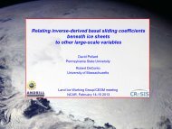
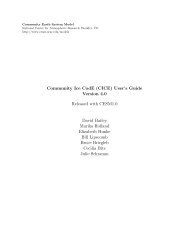
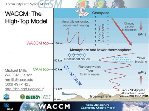
<strong>WACCM</strong>: <strong>The</strong><br />
<strong>High</strong>-<strong>Top</strong> <strong>Model</strong><br />
<strong>WACCM</strong> top<br />
Michael Mills<br />
<strong>WACCM</strong> Liaison<br />
mmills@ucar.edu<br />
(303) 497-1425<br />
http://bb.cgd.ucar.edu/<br />
CAM top 40 km<br />
Ozone Layer<br />
Jarvis, “Bridging the<br />
Atmospheric Divide”,<br />
Science, 293, 2218, 2001
<strong>WACCM</strong> Additions to CAM<br />
• Extends from surface to 5.1x10 -6 hPa (~150 km), with 66 vertical levels<br />
• Detailed neutral chemistry model for the middle atmosphere,<br />
• catalytic cycles affecting ozone<br />
• heterogeneous chemistry on PSCs and sulfate aerosol<br />
• heating due to chemical reactions<br />
• <strong>Model</strong> of ion chemistry in the mesosphere/lower thermosphere (MLT), ion drag,<br />
auroral processes, and solar proton events<br />
• EUV and non-LTE longwave radiation parameterizations<br />
• Imposed QBO, based on cyclic, fixed-phase, or observed winds<br />
• Volcanic aerosol heating calculated explicitly<br />
• Gravity wave drag deposition from vertically propagating GWs generated by<br />
orography, fronts, and convection<br />
• Molecular diffusion and constituent separation<br />
• <strong>The</strong>rmosphere extension (<strong>WACCM</strong>-X) to ~500 km
<strong>WACCM</strong> Motivation<br />
Roble, Geophysical Monograph, v. 123, p. 53, 2000<br />
• Coupling between atmospheric layers:<br />
• Waves transport energy and momentum from the lower<br />
atmosphere to drive the QBO, SAO, sudden warmings,<br />
mean meridional circulation<br />
• Solar inputs, e.g. auroral production of NO in the mesosphere and<br />
downward transport to the stratosphere<br />
• Stratosphere-troposphere exchange<br />
• Climate Variability and Climate Change:<br />
• What is the impact of the stratosphere on tropospheric variability?<br />
• How important is coupling among radiation, chemistry, and circulation?<br />
(e.g., in the response to O3 depletion or CO2 increase)<br />
• Response to solar variability: impacts mediated by chemistry?<br />
• Interpretation of Satellite Observations
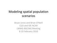
<strong>CESM</strong>-<strong>WACCM</strong> component configurations<br />
CAM<br />
specified chemistry<br />
free-running<br />
specified dynamics<br />
free-running<br />
atmosphere ocean<br />
<strong>WACCM</strong><br />
static<br />
(pre-industrial or<br />
present-day)<br />
transient<br />
free-running<br />
data<br />
observations<br />
climatology<br />
land sea ice<br />
data<br />
observations<br />
climatology<br />
freerunning<br />
data<br />
observations<br />
climatology
50N<br />
EQ<br />
50S<br />
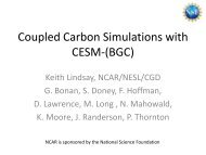
Stratospheric Sulfate Surface Area Density Climatology<br />
50N<br />
EQ<br />
50S<br />
El Chichón<br />
17°N, 93°W<br />
Agung<br />
8°S, 115°E<br />
Sulfate Surface Area Density, 43 hPa<br />
Mt Pinatubo:<br />
15°N, 120°E<br />
1960 1970 1980 1990 2000 2010<br />
Krakatau:<br />
6°S, 105°E,<br />
27-28 Aug 1883<br />
1880 1885 1890 1895 1900 1905 1910<br />
Santa<br />
Maria:<br />
14°N,<br />
91°W,<br />
24 Oct.<br />
1902<br />
• Observations<br />
used: SAGE I,<br />
SAGE II, SAM II,<br />
and SME<br />
instruments.<br />
• Non-volcanic<br />
periods filled<br />
with monthly<br />
mean of<br />
1998-2002<br />
values.<br />
• Used Pinatubo<br />
aerosol for<br />
Krakatau and<br />
Santa Maria.
Krakatoa 1883<br />
Krakatoa 1883<br />
Santa Maria 1902<br />
Santa Maria 1902<br />
Agung 1963<br />
Agung 1963<br />
Pinatubo 1991<br />
Chichón 1982<br />
Chichón 1982<br />
Pinatubo 1991<br />
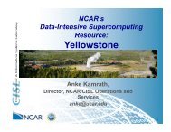
Surface Temperature Anomalies<br />
normalized to 1961-90<br />
—CCSM-CAM4 1deg<br />
—<strong>WACCM</strong>4 Pre-Indusrtrial<br />
—<strong>WACCM</strong>4 20th Century<br />
—<strong>WACCM</strong>4 1955-2005<br />
—Observations (HadCRUT3)<br />
Krakatoa 1883<br />
Santa Maria 1902<br />
Agung 1963<br />
Chichón 1982<br />
Pinatubo 1991
Volcanic heating in <strong>WACCM</strong><br />
2°N<br />
Surface Area (cm 2 cm -3 )<br />
Sulfate Mass (µg m -3 )<br />
Multiple aerosol independent<br />
parameters derived from<br />
observations used as inputs.<br />
2°N 2°N<br />
Effective Radius (cm)
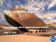
D12305 TILMES ET AL.: IMPACT OF THE GEOENGINEERED AEROSOLS D12305<br />
Volcanic heating in <strong>WACCM</strong><br />
D12305 TILMES ET AL.: IMPACT OF THE 30 GEOENGINEERED hPa occurred after AEROSOLS 1991 for both the differencesD12305 in the<br />
simulations (black line) and radiosonde anomalies (grey<br />
30 line) hPa (Figure occurred 1). For afterall 1991 three forpressure both thelevels, differences temperature in the<br />
simulations anomalies<br />
Temperature<br />
agree (blackwell line) between and radiosonde model<br />
anomalies<br />
and anomalies observations. (grey<br />
line) <strong>The</strong>refore, (Figurewe 1). expect For alla three reliable pressure response levels, of temperature the aerosol<br />
anomalies heating in the agree model well runbetween when using model geoengineered and observations. volcanic-<br />
<strong>The</strong>refore, sized aerosols. we expect a reliable response of the aerosol<br />
heating in the model run when using geoengineered volcanicsized<br />
2.2. aerosols. Setup of the Future Control and Geoengineering<br />
<strong>Model</strong> Runs<br />
pressures in the lower<br />
2.2. [14] Setup We performed of the Future two simulations Control and to analyze Geoengineering the impact<br />
<strong>Model</strong> of geoengineered Runs aerosols on the tropospheric and stratospheric<br />
[14] We dynamics, performed andtwo stratospheric simulations chemistry. to analyze<strong>The</strong> thecontrol, impact<br />
of or ‘‘baseline’’ geoengineered model aerosols run, is on initialized the tropospheric as a REF2 and model strato- run,<br />
spheric following dynamics, the CCMVal and stratospheric definition [Eyring chemistry. et al., <strong>The</strong> 2006],and control,<br />
or covers ‘‘baseline’’ the period modelbetween run, is initialized 2010 and as a2050. REF2 model Increasing run,<br />
following greenhousethe gases, CCMVal baseddefinition on the IPCC [Eyring A1Betscenario al., 2006],and [IPCC,<br />
covers 2007], are theincluded period in between this simulation, 2010 and as well 2050. as Increasing changes in<br />
greenhouse anthropogenic gases, halogen basedemissions. on the IPCC Initialized A1B scenario SAD and [IPCC, the<br />
2007], resulting areHincluded 2SO4 mass in this in the simulation, model are as prescribed well as changes usingina anthropogenic climatology for halogen a nonvolcanic emissions. Initialized period from SADSAGE and the II<br />
resulting [Thomason H et al.,<br />
2SO4 mass 1997]. in the model are prescribed using a<br />
climatology [15] <strong>The</strong> geoengineering for a nonvolcanic model run period is set from up identically SAGE to II<br />
[Thomason the baselineet run al., between 1997]. 2010 and 2020. However, starting<br />
in[15] the year <strong>The</strong> geoengineering 2020, the SAD model is increased run isfrom set upbackground identically to to<br />
the an enhanced, baseline run fixed between SAD2010 distribution. and 2020. This However, SAD isstarting calcu-<br />
in lated the from year 2020, the SO the4 SAD distribution is increased derived frominbackground the study of to<br />
an Rasch enhanced, et al. [2008b]. fixed SAD Rasch distribution. et al. [2008b] Thisused SADtheisNCAR calculated<br />
CAM from model thetoSO derive<br />
4 distribution aerosol distributions derived in the for study different of<br />
Rasch scenarios, et al. with [2008b]. varying Rasch amounts et al. of [2008b] sulfur used injection the NCAR in the<br />
CAM tropics,<br />
Figure model two<br />
1.<br />
different-sized toTemperature derive aerosol aerosol<br />
difference distributions types,<br />
between<br />
and two forthe different<br />
REF1.3v<br />
Pinatubo 1991<br />
Pinatubo 1991<br />
calculated with <strong>WACCM</strong> (black<br />
lines) and observed (grey lines) at<br />
stratosphere (Tilmes et al., 2009)<br />
Pinatubo 1991<br />
<strong>Model</strong> Run<br />
[14] We p<br />
of geoengin<br />
spheric dyn<br />
or ‘‘baseline<br />
following th<br />
covers the<br />
greenhouse<br />
2007], are i<br />
anthropogen<br />
resulting H 2<br />
climatology<br />
[Thomason<br />
[15] <strong>The</strong> g<br />
the baseline<br />
in the year 2<br />
an enhance<br />
lated from<br />
Rasch et al.<br />
CAM mode<br />
scenarios, w<br />
tropics, two<br />
CO 2 conditi<br />
al. [2008b],<br />
into a prese<br />
sols are assu<br />
astandardd<br />
effective rad<br />
[16] <strong>The</strong><br />
is an appro<br />
size spectru<br />
ulation time<br />
scheme (in<br />
aerosols alr<br />
by Rasch et<br />
distribution<br />
considered<br />
Tilmes et a
Grading of Chemistry in CCMs: Chapter 6 of the<br />
SPaRC CCMVal<br />
• CCMs were evaluated on<br />
their ability to represent longlived<br />
constituents<br />
(precursors) and short-lived<br />
substances (radicals).<br />
• <strong>WACCM</strong> graded out high in<br />
all categories (i.e., grade of 1<br />
is the highest possible).<br />
• This is a reflection of the:<br />
1) completeness of the<br />
chemical processes<br />
included<br />
2) accuracy of photolysis<br />
rates (J’s)<br />
3) and accuracy of the<br />
numerical solution<br />
approach.<br />
SPARC CCMVal, Report on the Evaluation of Chemistry-Climate <strong>Model</strong>s, V.Eyring, T. G. Shepherd, D. W. Waugh<br />
(EDs.), SPARC Reprot No.4, WCRP-X, WMO/TD-No. X, http://www.atmosp.physics.utoronto.ca/SPARC, 2010.
Temperature<br />
<strong>WACCM</strong> Heterogeneous Chemistry Module<br />
>200 K<br />
188 K<br />
(T sat)<br />
185 K<br />
(T nuc)<br />
Sulfate Aerosols (H 2O, H 2SO 4) - LBS<br />
k=1/4*V*SAD*γ (SAD from SAGEII)<br />
Sulfate Aerosols (H 2O, HNO 3, H 2SO 4) - STS<br />
<strong>The</strong>rmo. <strong>Model</strong> (Tabazadeh)<br />
Nitric Acid Hydrate (H 2O, HNO 3) – NAT<br />
R NAT = ƒ {Log Normal Size; # particles cc;<br />
width distribution; condensed phase HNO 3}<br />
ICE (H 2O, with NAT Coating)<br />
R ice= 10-30 μm<br />
?<br />
R lbs = 0.1 μm<br />
R sts = 0.5 μm
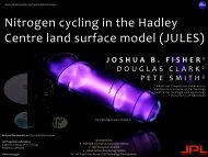
<strong>WACCM</strong> Ozone Trend: CCMVal and WMO<br />
Antarctic Spring <strong>WACCM</strong><br />
Redrawn from: Austin, J., et al., J. Geophys. Res., in press., 2010.<br />
does better<br />
than most<br />
models at<br />
calculating<br />
the evolution<br />
of the ozone<br />
hole.
Antarctic sea-ice extent<br />
CCSM4 (CAM4)<br />
-- Pre-Industrial<br />
— 1979-2005<br />
<strong>WACCM</strong>4<br />
-- Pre-Industrial<br />
— 1979-2005<br />
Observed 1979-2005 ave<br />
-- ice-ocean hindcast<br />
— Satellite<br />
CCSM4 (CAM)<br />
dashed lines:<br />
(1960-1979 ave) - PI<br />
solid lines:<br />
(1979-2005 ave) - PI<br />
<strong>WACCM</strong>4<br />
<strong>The</strong> more realistic ozone loss in <strong>WACCM</strong> drives changes in winds that enhance<br />
sea-ice loss, producing sea-ice extent closer to modern observations.
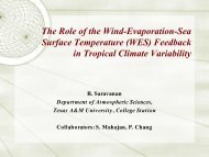
Acceleration of the Brewer–Dobson Circulation due to Increases in Greenhouse Gases<br />
L OF THE ATMOSPHERIC SCIENCES VOLUME<br />
Garcia and Randel, J. Atmos. Sci., vol. 65 (8), pp. 2731-2739, 2008.<br />
65<br />
and lower stratopper<br />
stratosphere<br />
sphere to enhanced and therere<br />
were made at<br />
5° longitude. <strong>The</strong><br />
idation activity of<br />
Role subtropics in Climate<br />
scribed in detail<br />
(specifically for<br />
• faster circulation in<br />
greenhouse world due<br />
propagation of wave<br />
activity into the lower<br />
stratosphere and its<br />
dissipation in the<br />
• changes in meridional<br />
temperature gradient<br />
affect zonal winds,<br />
which change the<br />
regions where waves<br />
dissipate, increasing<br />
momentum deposition<br />
of three ensemble<br />
rst, or reference<br />
ive” simulation of<br />
with sea surface<br />
HG and halogen<br />
<strong>The</strong> second simu-<br />
20th<br />
Century<br />
Age of Air (y),<br />
~10 hPa, tropics<br />
Future,<br />
increasing GHGs<br />
Future,<br />
fixed GHGs
Impact of geoengineered aerosols on the troposphere and stratosphere<br />
Tilmes et al., J. Geophys. Res., vol. 114, pp. 12305, 2009.<br />
• ~5 years for adjustment of temperatures<br />
• Constant temperature offset<br />
Annual mean, zonally averaged global temperature difference between present day (2010–<br />
uture (2040–2050) for (a) the baseline run and (b) the geoengineering run. (c) Annual mean,<br />
raged global temperature difference between geoengineering and baseline runs for future<br />
) conditions. Hatched areas are not significant at 95% level based on Student’s t test.<br />
of geoengineered aerosols is constant.<br />
d in the case of geoengineering would<br />
elmed by increasing greenhouse gases<br />
ission scenario, unless the content of<br />
tosphere were adjusted. In our case,<br />
ys global warming by approximately<br />
appreciated from Figure 4. <strong>The</strong>refore,<br />
of 2 Tg S per year of volcanic-sized<br />
Temperature:<br />
Geoengineering - Baseline<br />
• <strong>The</strong> fixed amount of sulfur cools the Earth’s<br />
surface by ~0.9 K (Tropics), ~1.2 K (Global)<br />
aerosols is shown to counteract global warming through<br />
about 2050 with respect to the situation in 2010.<br />
• Delay of global warming by ~ 40 years<br />
• Dependence on continuous injection of sulfur<br />
4. Impact of Geoengineered Aerosols on Surface<br />
Temperatures and Climate<br />
[28] Increasing greenhouse gases result in increasing<br />
tropospheric and decreasing stratospheric temperatures.<br />
T anomaly (K) Baseline / Geoengineering<br />
40 km<br />
year 2020 2030 2040 2050<br />
30 km<br />
year 2020 2030 2040 2050<br />
10 km<br />
year 2020 2030 2040 2050<br />
surface<br />
year 2020 2030 2040 2050
Altitude (km)<br />
Impact of geoengineered aerosols on the troposphere and stratosphere<br />
Tilmes et al., J. Geophys. Res., vol. 114, pp. 12305, 2009.<br />
Impacts of geoengineering on ozone<br />
in the lower stratosphere compared to<br />
arcia and Randel, 2008]. Further, the<br />
D12305 TILMES ET AL.: IMPACT OF THE GEOENGINEERED AEROSO<br />
Baseline –Geoengineering<br />
Latitude<br />
Difference of annual mean zonally averaged global ozone values between present day (2010–<br />
future (2040–2050) for (a) the baseline run and (b) the geoengineering run. (c) Difference of<br />
n zonally averaged global ozone values between geoengineering and baseline runs for future<br />
0) conditions. Hatched areas are not significant at 95% level based on Student’s t test.<br />
tion is discussed below for the tropics, midlatitudes and<br />
polar regions.<br />
Impact of geoengineering
Massive global ozone loss predicted following regional nuclear conflict<br />
Mills et al., PNAS, vol. 105, pp. 5307, 2008<br />
• <strong>WACCM</strong> input: new<br />
estimates of smoke<br />
produced by fires in<br />
contemporary cities<br />
following a regional<br />
nuclear war between<br />
India and Pakistan<br />
• Solar radiation heats<br />
the soot, lofting it to<br />
the stratopause,<br />
heating the the entire<br />
stratosphere for 10<br />
years, altering<br />
reaction rates<br />
affecting ozone.<br />
• Calculated ozone losses exceed 20% globally, 25-45% at midlatitudes, and 50-70% at northern high<br />
latitudes persisting for 5 years, with substantial losses continuing for 5 additional years. Column ozone<br />
amounts remain below that which defines the Antarctic ozone hole everywhere outside of the tropics.
Nuclear winter in <strong>WACCM</strong>4<br />
Black Carbon Input<br />
150-300 hPa<br />
GISS <strong>Model</strong>E<br />
(Robock et al., 1997)<br />
Year<br />
<strong>WACCM</strong>4<br />
GISS <strong>Model</strong>E<br />
Year<br />
<strong>WACCM</strong>4<br />
GISS <strong>Model</strong>E<br />
<strong>WACCM</strong>4
<strong>WACCM</strong> and CAM-Chem Customer Support<br />
CGD Forum: http://bb.cgd.ucar.edu/<br />
Mike Mills<br />
<strong>WACCM</strong> Liaison<br />
mmills@ucar.edu<br />
(303) 497-1425<br />
Simone Tilmes<br />
CAM-Chem Liaison<br />
tilmes@ucar.edu<br />
(303) 497-1425