R7.1 Polymerization

10 11 lb/yr 

Everyday Examples 

Polyethylene 

Softdrink cups 

Sandwich bags 

Poly (vinyl chloride) 

Pipes 

Shower curtains 

Tygon tubing 

Poly (vinyl acetate) 

Chewing gum 

Sec. R7.1 Polymerization 

R7.1 Polymerization 

Polymers are finding increasing use throughout our society. Well over 100 billion 

pounds of polymer are produced each year, and it is expected that this figure 

will double in the coming years as higher-strength plastics and composite materials 

replace metals in automobiles and other products. Consequently, the field 

of polymerization reaction engineering will have an even more prominent place 

in the chemical engineering profession. Because there are entire books on this 

field (see Supplementary Reading), 

it is the intention here to give only the most 

rudimentary thumbnail sketch of some of the principles of polymerization. 

A polymer is a molecule made up of repeating structural (monomer) 

units. For example, polyethylene is used for such things as tubing, and repeating 

units of ethylene are used to make electrical insulation: 

nCH2—CH2 ⎯⎯→ — [ CH — CH — ] 

where n may be 25,000 or higher. 

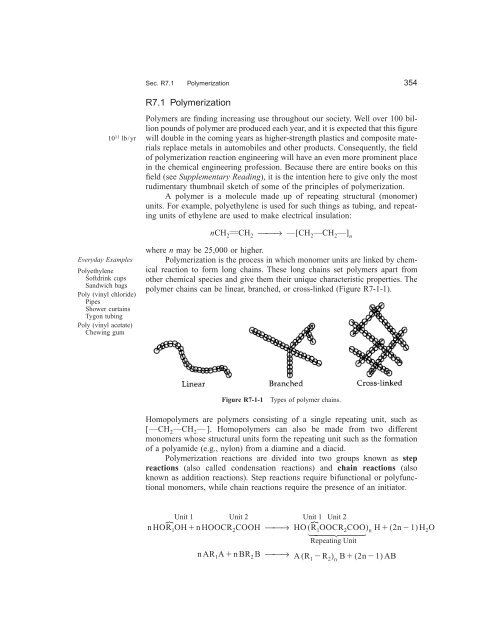
Polymerization is the process in which monomer units are linked by chemical 

reaction to form long chains. These long chains set polymers apart from 

other chemical species and give them their unique characteristic properties. The 

polymer chains can be linear, branched, or cross-linked (Figure R7-1-1). 

Figure R7-1-1 Types of polymer chains. 

Homopolymers are polymers consisting of a single repeating unit, such as 

[ —CH2—CH2— ]. Homopolymers can also be made from two different 

monomers whose structural units form the repeating unit such as the formation 

of a polyamide (e.g., nylon) from a diamine and a diacid. 

Polymerization reactions are divided into two groups known as step 

reactions (also called condensation reactions) and chain reactions (also 

known as addition reactions). Step reactions require bifunctional or polyfunctional 

monomers, while chain reactions require the presence of an initiator. 

Unit 1 Unit 2 Unit 1 Unit 2 

nHOR1OH� nHOOCR2COOH ⎯⎯→ HO( R1OOCR2COO) 

n H � ( 2n 

� 1) 

H2O 

} 

nAR 

1 

2 

} 

2 

⎧ 

⎪ 

⎪ 

⎨ 

⎪ 

⎪ 

⎩ 

n 

Repeating Unit 

A� nBR2B 

⎯⎯→ A( R � R ) 

1 

2 n 

B 2n 1 � ( ) AB 

� 

354

Categories 

of Copolymers 

355 

Chap. 

Copolymers are polymers made up of two or more repeating units. There are 

five basic categories of copolymers that have two different repeating units Q 

and S. They are 

1. Alternating: 

–Q–S–Q–S–Q–S–Q–S–Q–S– 

2. Block: 

–Q–Q–Q–Q–Q–S–S–S–S–S– 

3. Random: 

–Q–Q–S–Q–S–S–Q–S–S–S– 

4. Graft: 

–Q–Q–Q–Q–Q–Q–Q–Q–Q–Q– 

S–S–S–S–S–S– 

5. Statistical (follow certain addition laws) 

Examples of each can be found in Young and Lovell. 1 

R7.1.1 Step Polymerization 

Step polymerization requires that there is at least a reactive functional group 

on each end of the monomer that will react with functional groups with other 

monomers. For example, amino-caproic acid 

has an amine group at one end and a carboxyl group at the other. Some common 

functional groups are —OH , —COOH , —COCl , —NH2 . 

In step polymerization the molecular weight usually builds up slowly 

Dimer 

For the preceding case the structural unit and the repeating unit are the same. 

Letting A�H , R� NH—R1—CO, 

and B�OH , AB � H2O. 

We can 

write the preceding reaction as 

1 

Dimer 

Trimer 

Tetramer 

Pentamer 

Hexamer 

R. J. Young and P. A. Lovell, 

& Hall, 1991). 

NH2—CH ( 2) 

5 —COOH 

Structural Unit Repeating Unit 

2H ( NH—R—CO) 

OH ⎯⎯→ H ( NH—R—CO) 

2 OH� H2O 

⎫ 

⎪ 

⎪ 

⎬ 

⎪ 

⎪ 

⎭ 

ARB � ARB 

ARB � A—R2—B ARB � A—R3—B A—R2—B � A—R2—B ARB � A—R4—B A—R2—B � A—R3—B ARB � A—R5—B A—R2—B � A—R4—B A—R3—B � A—R3—B ⎫ 

⎪ 

⎪ 

⎬ 

⎪ 

⎪ 

⎭ 

⎯⎯→ A—R2—B� 

AB 

⎯⎯→ A—R3—B� 

AB 

⎯⎯→ A—R4—B� 

AB 

⎯⎯→ A—R4—B� 

AB 

⎯⎯→ A—R5—B� 

AB 

⎯⎯→ A—R5—B� 

AB 

⎯⎯→ A—R6—B� 

AB 

⎯⎯→ A—R6—B� 

AB 

⎯⎯→ A—R6—B� 

AB 

Introduction to Polymers, 

2nd ed. (New York: Chapman


etc. 

overall: 

n 

NH 

2 

RCOOH ⎯⎯→ H(NHRCO) OH � (n � 

n ARB 

⎯⎯→ A—Rn—B 

n 

� 

( n � 1)AB 

1)H2O 

We see that from tetramers on, the –mer can be formed by a number of different 

pathways. 

The A and B functional groups can also be on different monomers such as 

the reaction for the formation of polyester (shirts) from diols and dibasic acids. 

Unit 1 Unit 2 Unit 1 Unit 2 

⎩ 

⎪ 

n AR1A 

⎨ 

⎪ 

⎧ 

⎪ 

⎨ 

⎪ 

⎧ 

⎪ 

n HOR1OH� 

n HOOCR2COOH 

⎯⎯→ HO( R1OOCR2COO) 

n H � ( 2n 

� 1) 

H2O 

Repeating Unit 

} 

By using diols and diacids we can form polymers with two different structural 

units which together become the repeating unit. An example of an AR1A 

plus 

BR2B 

reaction is that used to make Coca-cola bottles (i.e., terephthalic acid 

plus ethylene glycol to form poly [ethylene glycol terephthalate]). 

When discussing the progress of step polymerization, it is not meaningful 

to use conversion of monomer as a measure because the reaction will still 

proceed even though all the monomer has been consumed. For example, if the 

monomer A—R—B has been consumed. The polymerization is still continuing 

with 

A—R2—B� A—R3—B ⎯⎯→ A—R5—B� 

AB 

A—R5—B� 

A—R5—B 

⎯⎯→ A—R10—B� 

AB 

because there are both A and B functional groups that can react. Consequently, 

we measure the progress by the parameter p, which is the fraction of functional 

groups, A, B, that have reacted. We shall only consider reaction with 

equal molar feed of functional groups. In this case 

p Mo � M fraction of functional groups of either A or B that 

� ------------------ � 

have reacted 

M o 

� 

n BR2 

B ⎯⎯→ 

As an example of step polymerization, consider the polyester reaction in which 

sulfuric acid is used as a catalyst in a batch reactor. Assuming the rate of disappearance 

is first order in A, B, and catalyst concentration (which is constant 

for an externally added catalyst). The balance on A is 

} 

⎩ 

⎧ 

⎪ 

⎪ 

⎨ 

⎪ 

⎪ 

A( R � R ) 

M concentration of either A or B functional groups (mol/dm3 � 

) 

�d[ 

A] 

---------------- � k[ A] 

[ B] 

dt 

1 

2 n 

⎩ 

B 2n1 

� ( ) AB 

� 

356 

(R7.1-1)

Degree 

of polymerization 

357 

For equal molar feed we have 

[A] � [B] � M 

dM 

------- kM 

dt 

2 � � 

Chap. 

M � -------------------- 

(R7.1-2) 

1 � Mokt In terms of the fractional conversion of functional groups, p, 

1 

------------ � M (R7.1-3) 

1 � p 

okt� 1 

The number-average degree of polymerization, Xn , is the average number of 

structural units per chain: 


The number-average molecular weight, Mn, 

is just the average molecular 

weight of a structural unit, Ms , times the average number of structural unit per 

chain, , plus the molecular weight of the end groups, : 

Since 

Xn 

M 

eg 

Meg 

is usually small (18 for the polyester reaction), it is neglected and 


In addition to the conversion of the functional groups, the degree of polymerization, 

and the number average molecular weight we are interested in the 

distribution of chain lengths, n (i.e. molecular weights ). 

M 

n 

Example R7–1 Determining the Concentrations of Polymers 

for Step Polymerization 

Determine the concentration and mole fraction of polymers of chain length j in 

terms of initial concentration of ARB, Mo, 

the concentration of unreacted functional 

groups M, 

the propagation constant k and time t. 

Solution 

Letting P1 �A—R—B , P 2 �A—R2—B , … , P j �A—Rj—B 

and omitting the 

water condensation products AB for each reaction we have 

Reaction Rate Laws 

(1) 2P1 

→ P2 

(2) P1 

� P2 

→ P3 

Xn 

M o 

1 

� ------------ 

1 � p 

Mn � Xn Ms � Meg Mn � Xn Ms 

r 2 

1P1 2 

�r1P1 �2kP1, r1P2 ��-------- � kP1 2 

�r2P1 ��r2P2�r2P3�2kP1P2


(3) P1 

� P3 

→ P4 

(4) P2 

� P2 

→ P4 

358 

The factor of 2 in the disappearance term (e.g., �r3P3 � 2kP1P3 ) comes about 

because there are two ways A and B can react. 

P1 

is 

The net rate of reaction of P1, 

P2 

and P3 

for reactions (1) through (4) are 

2 

r1 � rP1 � �2kP1� 2kP1P2 �2kP1P3 

( RE7.1-1) 

( RE7.1-2) 

( RE7.1-3) 

If we continue in this way, we would find that the net rate of formation of the 

( RE7.1-4) 

However, we note that is just the total concentration of functional groups of 

either A or B, which is M 

⎛ � ⎞ 

⎜M�Pj. ⎝ � ⎟ 

⎠ 

( RE7.1-5) 

Similarly we can generalize reactions (1) through (4) to obtain the net rate of formation 

of the j-mer, for j� 2 . 

(RE7.1-6) 

For a batch reactor the mole balance on P 1 and using Equation (RE7.1-2) to eliminate 

M gives 

which solves to 

�r3P1 ��r3P3�r3P4�2kP1P3 r 2 

4P2 2 

�r4P2 �2kP2, r4P4 ��-------- � kP2 2 

A�Rn�B A�Rm�B 2 

r2 � rP2 � kP1� 2kP1P2 �2kP2 

r3 � rP3 � 2kP1P2 �2kP1P3 �2kP2P3 

� 

P � j 

j�1 

r P1 

� � 

j�1 

r P1 

� 

j�1 

r j � k P 

� 

i�1 

� 

2kP1 P � j 

j�1 

�2kP1 

M 

i 

P j�i 

� 

2 

2kPj 

M 

dP1 -------- �2kP1 M 2kP1 dt 

Mo 

1 � M kt 

-------------------- 

� �� 

P1 � 

M o 

⎛ 1 ⎞ 

⎜-------------------- ⎟ 

⎝1� Mokt⎠ 

2 

o 

(RE7.1-7) 

(RE7.1-8)

359 

Having solved for 

Recalling 

P1 

we can now use rj 

to solve successively for Pj 

The mole fraction of polymer with a chain length j is just 

Recalling M � 

Mo(1 

� p), 

we obtain 

Chap. 

(RE7-1.9) 

(RE7.10) 

( RE7.1-11) 

( RE7.1-12) 

( RE7.1-13) 

(R.1-6) 

This is the Flory–Schulz distribution. We discuss this distribution further after 

we discuss chain reactions. 

7.1.2 Chain Polymerizations Reactions 

Chains (i.e., addition) polymerization requires an initiator ( I) 

and proceeds by 

adding one repeating unit at a time. 

2 

dP2 2 

-------- �r2�kP1� 2kP2 M 

dt 

4 

2 ⎛ 1 ⎞ ⎛ 1 

� kMo ⎜-------------------- ⎟ �2M 

ok 

⎜-------------------- 


⎝1 

� Mokt 

with P2 

� 0 at t � 0 

2 

⎛ 1 ⎞ 

P2 Mo ⎜-------------------- ⎟ 


Continuing we find that, in general2 

Mokt 

1 � Mokt 

-------------------- 

⎛ ⎞ 

� 

⎜ ⎟ 

⎝ ⎠ 

p Mo � M 

� ------------------ 

M o 

P j 

� 

M o 

⎛ 1 ⎞ 

⎜-------------------- ⎟ 


N. A. Dotson, R. Galván, R. L. Lawrence, and M. Tirrell, Polymerization Process 

Modeling, 

New York: VCH Publishers (1996). 

2 

Mokt 

1 � Mokt 

-------------------- 

⎛ ⎞ 

⎜ ⎟ 

⎝ ⎠ 

P j Mo ( 1� p) 

2 p j�1 

� 

y j 

P j 

� ---- 

M 

y j ( 1 � p)pj�1 

� 

I� M ⎯⎯→ 

M� R1 

⎯⎯→ 

M� R2 

⎯⎯→ 

M� R3 

⎯⎯→ 

M� R4 

⎯⎯→ 

R 

1 

R 

2 

R 

3 

R 

4 

R , 

etc. 

5 

j�1


Here the molecular weight in a chain usually builds up rapidly once a chain is 

initiated. The formation of polystyrene, 

n C 6 H5CH—CH2 

⎯⎯→ [ —CHCH2— 

] 

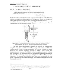
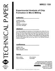
is an example of chain polymerization. A batch process to produce polystyrene 

for use in a number of molded objects is shown in Figure R7.1-2. 

Styrene 

monomer 

Filter 

Circulating 

hot water 

Circulating 

hot water 

Reflux 

condenser 

Agitated 

prepolymerization 

kettle 

C6H5 

Plate & frame press 

Crusher 

We can easily extend the concepts described in the preceding section to 

polymerization reactions. In this section we show how the rate laws are formulated 

so that one can use the techniques developed in Chapter 6 for multiple 

reactions to determine the molecular weight distribution and other properties. 

In the material that follows we focus on free-radical polymerization. 

n 

Screens 

Polystyrene 

granules 

Fogler/Prenhall/F7.4 

Figure R7.1-2 Batch bulk polystyrene process. (From Chemical Reactor Theory, 

p. 543, Copyright © 1977, Prentice Hall. Reprinted by permission of Prentice Hall, 

Upper Saddle River, NJ) 

360

Polystyrene 

Coffee Cups 

361 

R7.1.2.1 Steps in Free-Radical Polymerization 

Chap. 

The basic steps in free-radical polymerization are initiation, propagation, chain 

transfer, and termination. 

Initiation. Chain polymerization reactions are different because an initiation 

step is needed to start the polymer chain growth. Initiation can be achieved by 

adding a small amount of a chemical that decomposes easily to form free radicals. 

Initiators can be monofunctional and form the same free radical: 

k0 

Initiation I2 ⎯⎯→ 2 I 

Propagation 

Assumption of equal 

For example, 2,2-azobisisobutyronitrile: 

or they can be multifunctional and form different radicals. Multifunctional initiators 

contain more than one labile group3 

[e.g., 2,5 dimethyl-2,5-bis(benzoylperoxy)hexane]. 

For monofunctional initiators the reaction sequence between monomer M 

and initiator I is 

For example, 

Propagation. The propagation sequence between a free radical 

monomer unit is 

In general, 

3 

( CH3) 2CN—NC( CH3) 2 ⎯⎯→ 2 ( CH ) 

R 

1 

with a 

J. J. Kiu and K. Y. Choi, Chem. Eng. Sci., 43, 

65 (1988); K. Y. Choi and G. D. Lei, 

AIChE J., 33, 

2067 (1987). 

3 2 

C � 

CN CN CN 

k 

i 

I� M ⎯⎯→ R 1 

( CH3) 2C � � CH2—CHCl ⎯⎯→ ( CH3) 

2 

� N2 

C CH C � 

CN CN Cl 

k 

p 

R1 � M ⎯⎯→ R 2 

kp 

R2 

� M ⎯⎯→ R 3 

reactivity R j� M ⎯⎯→ R j 

k 

p 

�1 

2 

H

Chain 


For example, 

( CH3) 2CCH ( 2CHCl) 

j CH2C � � CH2C � CHCl ⎯⎯→ ( CH3) 

CN Cl 

The specific reaction rates kp 

are assumed to be identical for the addition of 

each monomer to the growing chain. This is usually an excellent assumption 

once two or more monomers have been added to R1 

and for low conversions of 

monomer. The specific reaction rate is often taken to be equal to . 

k 

i 

Chain Transfer. The transfer of a radical from a growing polymer chain can 

occur in the following ways: 

1. Transfer to a monomer: 

R j 

k 

p 

362 

Here a live polymer chain of j monomer units tranfers its free radical 

to the monomer to form the radical R1 

and a dead polymer chain of j 

monomer units. 

2. Transfer to another species: 

3. Transfer of the radical to the solvent: 

H 

�M ⎯⎯→ P j� 

R1 

transfer R j C ⎯⎯→ P j 

R j 

k 

m 

kc 

� � 

k 

s 

The species involved in the various chain transfer reactions such 

as CCl3� 

and C6H5CH2� 

are all assumed to have the same reactivity as 

R1. 

In other words, all the R1’s 

produced in chain transfer reactions are 

taken to be the same. However, in some cases the chain transfer agent 

may be too large or unreactive to propagate the chain. The choice of 

solvent in which to carry out the polymerization is important. For 

example, the solvent transfer specific reaction rate ks 

is 10,000 times 

greater in CCl4 

than in benzene. 

The specific reaction rates in chain transfer are all assumed to 

be independent of the chain length. We also note that while the radicals 

R1 

produced in each of the chain transfer steps are different, they 

function in essentially the same manner as the radical R1 

in the propagation 

step to form radical . 

R 

2 

R 

1 

�S ⎯⎯→ P j � R1 

CCH ( CHCl) 

2 

2 

H 

j�1CH2C 

� 

CN Cl

Termination 

Initiation 

Propagation 

Transfer 

Termination 

363 

Termination. 

mechanisms: 

Chap. 

Termination to form dead polymer occurs primarily by two 

1. Addition (coupling) of two growing polymers: 

2. Termination by disproportionation: 

For example, 

R j 

The steps in free-radical polymerization reaction and the corresponding 

rate laws are summarized in Table R7.1-1. For the polymerization 

of styrene at 80�C 

initiated by 2,2-azobisisobutyronitrile, the 

rate constants4 

are 

k0 

� 1.4 � 10�3 

s�1 

R j 

kp 

� 4.4 � 102 

dm3/mol�s 

ks 

� 2.9 � 10�3 

dm3/mol�s 

� Rk ⎯⎯→ P j 

km 

� 3.2 � 10�2 

dm 3/mol�s 

kta 

� 1.2 � 108 

dm3/mol�s 

ktd 

� 0 

Typical initial concentrations for the solution polymerization of styrene are 

0.01 M for the initiator, 3 M for the monomer, and 7 M for the solvent. 

R7.1.2.2 Developing the Rate Laws for the Net Rate 

of Reaction 

We begin by considering the rate of formation of the initiator radical I. 

Because there will always be scavenging or recombining of the primary radicals, 

only a certain fraction f will be successful in initiating polymer chains. 

Because each reaction step is assumed to be elementary, the rate law for the 

formation of the initiator free radicals, r If, is 

�k 

4 D. C. Timm and J. W. Rachow, ACS Symp. Ser. 133, 122 (1974). 

k 

td 

k 

ta 

�Rk ⎯⎯→ P j� 

H H 

( CH3) 2CCH ( 2CHCl) 

j CH2C � C�CH2( CH2CHCl) k ( CH3) 2C CN Cl Cl CN 

H 

H 

(CH 3) 2C(CH 2CHCl) j CH � C�CH(CH 2CHCl) k(CH 3) 2 C 

P 

k 

CN Cl Cl 

CN

Rate of initiation 


Initiation: 

Propagation: 

Chain transfer to: 

Monomer: 

Another species: 

Solvent: 

Termination: 

Addition: 

Disproportionation: 

rIf 

� 2fk0( 

I2) 

where f is the fraction of initiator free radicals successful in initiating chaining 

and has a typical value in the range 0.2 to 0.7. The rate law for the formation 

of R1 

in the initiation step is 

rR1 

� �ri 

� ki 

( M)(I) (R7.1-7) 

Using the PSSH for the initiator free radical, I, we have 

rI � 2fk0(I2) � ki (M)(I) � 0 

2 fk0( I2) (I) � -------------------- 


( M)ki 

Then 

�ri � 2fk0(I2) (R7.1-9) 

Before writing the rate of disappearance of R1, we need to make a couple 

of points. First, the radical R1 can undergo the following termination sequence 

by addition. 

R 1 � R 1 

R 1 � R 2 

TABLE R7.1-1 

I 2 

I � M 

Rate Law 

Rj � M ⎯⎯→ R j�1 

�rj � kpMRj Rj � M ⎯⎯→ P j� 

R1 

�rmj � kmMRj Rj � C ⎯⎯→ P j� 

R1 

�rcj � kcCRj Rj � S ⎯⎯→ P j� 

R1 

�rsj � ksSRj R j � R k 

R j � R k 

k0 

⎯⎯→ 2 I 

ki 

⎯⎯→ R 1 

k 

p 

k 

m 

k 

c 

k 

s 

k 

ta 

⎯⎯→ P j 

k 

�k 

td 

⎯⎯→ P j� 

P 

k 

kta 

⎯⎯→ P 2 

kta 

⎯⎯→ P 3 

⎧ 

⎪ 

⎨ 

⎪ 

⎩ 

�rI2 rIf �ri � k0I 2 

� 2 fk0I2 � ki MI 

�r aj � k taR j R k 

�r dj � k tdR j R k 

364

Termination of R 1 

Net rate of 

disappearance of 

radicals of chain 

length one 

Net rate of 

disappearance of 

radicals of chain 

length j 

365 

In general, 

R1 

� Rj 

Chap. 

Consequently, the total loss of R1 

radicals in the preceding reactions is found 

by adding the loss of R1 

radicals in each reaction so that the rate of disappearance 

by termination addition is given by 

�r1t 

� k 

ta 

2 R1 �r1t 

� ktaR1 

⎯⎯→ P j 

� ktaR1R2 

� ktaR1R3 

� �� ktaR1Rj 

� �� 

� 

� 

j�1 

R j 

Free radicals usually have concentrations in the range 10�6 

to 10�8 

mol/dm3 . 

We can now proceed to write the net rate of disappearance of the free radical, 

R1. [R1 � (R1) � .] 

C R1 


In general, the net rate of disappearance of live polymer chains with j 

monomer units (i.e., length j ) for ( j � 2) is 


At this point one could use the techniques developed in Chapter 6 on multiple 

reactions to follow polymerization process. However, by using the PSSH, we 

can manipulate the rate law into a form that allows closed-form solutions for a 

number of polymerization reactions. 

First, we let R � be the total concentration of the radicals R j: 

R � � (R7.1-12) 

and kt be the termination constant kt � (kta � ktd). Next we sum Equation 

(R7.1-11) over all free-radical chain lengths from j � 2 to j � �, 

and then add 

the result to Equation (R7.1-10) to get 

k 

ta 

�1 

�r1 �ri k p R1 M kta R1 R j ktd 

R1 

R 

� 

� � � 

� 

� 

� k m M R � 

j�2 

j 

k 

c 

� 

� 

j�1 

� 

� 

C R � 

j�2 

j 

k 

s 

� 

� 

j�1 

� 

� 

S R 

j�2 

�r j k p MR ( j� R j�1) 

( kta� ktd)Rj R 

� 

� 

� 

� 

i�1 

�kMR �k�ksSRj m 

� 

� 

j�1 

j 

R j 

cCR j 

i 

j 

j

Total 

free-radical 

concentration 

Long-chain 

approximation 

(LCA) 


The total rate of termination is just 

�rj 

� �ri 

� kt( 

R�) 

2 

Using the PSSH for all free radicals, that is, 

concentration solves to 

j�1 

366 


�rj 

� 0, the total free-radical 


We now use this result in writing the net rate of monomer consumption. 

As a first approximation we will neglect the monomer consumed by monomer 

chain transfer. The net rate of monomer consumption, �rM, 

is the rate of consumption 

by the initiator plus the rate of consumption by all the radicals Rj 

in 

each of the propagation steps ( r ). 

p 

�rM 

� �ri � �rp � �ri � kpM We now use the long-chain approximation (LCA). The LCA is that the 

rate of propagation is much greater than the rate of initiation: 

Substituting for r p and r i,we obtain 

� 

� 

rt kt R� ( ) 2 � 

�ri kt R� � -------- � 

�k p MR � 

r p 

ri ---- � 1 

Consequently, we see that the LCA is valid when both the ratio of monomer 

concentration to initiator concentration and the ratio of k2 p to (k0 fkt) are high. 

Assume that the LCA gives 

� 

� 

j�1 

2k0 ( I2)f -------------------- 

k t 

k p 2k 0 f I 2 

� 

� 

j�1 

R j 

r p 

( ( ) � kt ) 1 2 

---- -------------------ri 

�ki MI 

� 

� � --------------------------------------------ki 

( 2k0 f( I2) � Mki ) 

M k2 

p 

� ------- --------------- 

1�2 I 2 k 

2 0 fkt

Rate of 

disappearance 

of monomer 

Rate of formation of 

dead polymers 

Monomer 

balance 

Initiator 

balance 

367 

Using Equation (R7.1-14) to substitute for 

monomer is 

The rate of disappearance of monomer, 

agation, : 

r 

p 

�rM � k p M R � 

�r M 

j�1 

Finally, the net rate of formation of dead polymer 

r P j 

The rate of formation of all dead polymers is 

rP 

� 0.5kta( 

R�) 

2 

R7.1.3 Modeling a Batch Polymerization Reactor 

Chap. 


R�, 

the rate of disappearance of 


�rM, 

is also equal to the rate of prop- 

Pj 

by addition is 


To conclude this section we determine the concentration of monomer as a 

function of time in a batch reactor. A balance on the monomer combined with 

the LCA gives 

� 

A balance on the initiator I2 

gives 

dM 

------- � k p M ∑ R j � k p MR� 

� 

dt 

Integrating and using the initial condition 

tion of the initiator concentration profile: 

� 

� 

� 

j 

k p MR� 

k p M 2k0 

( I2) 

f 

� -------------------- 

r p 

0.5k ta 

r P 

� �rM 

� 

k�j�1 

� 

k�1 

� 

� 

j�1 

r P j 

� dI2 ------- � 

k0 I2 dt 

k 

t 

Rk 

R j�k 

k 

p 

M 2k0 

( I2) 

f 

-------------------- 

k 

t 


I2 

� I20 

at t � 0, we obtain the equa


I2 

� I20 

exp( �k0t) 


Substituting for the initiator concentration in Equation (R7.1-18), we get 

dM 

------- �k p M 

dt 

Integration of Equation (R7.1-20) gives 

2k 

⎛ 0 I20 

f ⎞ 

� ⎜------------------ ⎟ 

⎝ kt 

⎠ 

M ⎛8k2 p fI20⎞ 

ln------ � ⎜------------------ ⎟ 

M0 ⎝ k0 kt ⎠ 

1 2 � 

368 



One notes that as t ⎯⎯→ � , there will still be some monomer left unreacted. 

Why? 

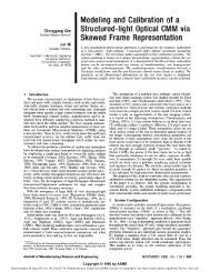
A plot of monomer concentration is shown as a function of time in 

Figure R7-5 for different initiator concentrations. 

M (mol/dm 3 ) 

3.000 

2.000 

1.000 

I 0 = 0.01 M 

The fractional conversion of a monofunctional monomer is 

X 

We see from Figure R7.1-3 that for an initiator concentration 0.001 M, 

the 

monomer concentration starts at 3 M and levels off at a concentration of 0.6 M, 

corresponding to a maximum conversion of 80%. 

M0 � M 

� 

------------------ 

M0 1�2 0.000 

0.000 20.000 40.000 60.000 

t (hr) 

⎛ k ⎞ 0 

exp ⎜�--- t⎟ 

⎝ 2 ⎠ 

⎛ k0 

t⎞ 

exp ⎜�------ ⎟�1 

⎝ 2 ⎠ 

I 0 = 0.00001 M 

I 0 = 0.0001 M 

I 0 = 0.001 M 

Fogler/Prenhall/F7 5 

80.000 100.000 

Figure R7.1-3 Monomer concentration as a functional time.

369 

Chap. 

Now that we can determine the monomer concentration as a function of 

time, we will focus on determining the distribution of dead polymer, Pj. 

The 

concentrations of dead polymer and the molecular weight distribution can be 

derived in the following manner. 5 The probability of propagation is 

Simplifying 


In the absence of chain transfer, the monomer concentration, M, 

can be determined 

from Equation (R7.1-22) and concentration of initiator, I2, 

from Equation 

(R7.1-19). Consequently we have � as a function of time. We now set 

to use in the Flory distribution. 

It can be shown that in the absence of termination by combination, the 

mole fractions yj 

and weight fraction wj 

are exactly the same as those for step 

polymerization. That is, we can determine the dead polymer concentrations 

and molecular weight distribution of dead polymer in free radial polymerization 

for the Flory distributions. For example, the concentration of dead polymer 

of chain length n is 

⎛ � ⎞ 

where ⎜ Pn is the total dead polymer concentration and 

⎝�⎟ ⎠ 


which is the same as the mole fraction obtained in step polymerization, i.e. 

Equation (R7.1-6). 

If the termination is only by disproportionation, the dead polymer Pj 

will 

have the same distribution as the live polymer . 

5 

n�2 

Rate of propagation 

� � ---------------------------------------------------------------------------------------------------- � -------------- 

Rate of propagation � Rate of termination � 

k p MR � 

� 

k p MR� ks SR� km MR� kcCR� kt R� ( ) 2 

� ----------------------------------------------------------------------------------------------------------- 

� � � � 

k p M 

� � ----------------------------------------------------------------------------------------------- 

� � � � ( ) 

k p M k m M k cC k s S 2k t k o f I 2 

� � p 

⎛ � ⎞ ⎛ � ⎞ 

Pn � yn ⎜ P � j⎟ 

� ⎜ P j 

⎝ ⎠ ⎝�⎟ ( 1 � p) 

⎠ 

j�2 

j�2 

yn ( 1 � p)pn�1 

� 

E. J. Schork, P. B. Deshpande, and K. W. Leffew, Control of Polymerization Reactor 

(New York: Marcel Dekker, 1993). 

R 

j 

pn�1 

r p 

r p rt


We will discuss the use of the Flory equation after we discuss molecular 

weight distributions. 

R7.1.4 Molecular Weight Distribution 

Although it is of interest to know the monomer concentration as a function of 

time (Figure R7.1-3), it is the polymer concentration, the average molecular 

weight, and the distribution of chain lengths that give a polymer its unique 

properties. Consequently, to obtain such things as the average chain length of 

the polymer, we need to determine the molecular weight distribution of radicals 

(live polymer), Rj, 

and then dead polymers Pj 

as well as the molecular 

weight distribution. Consequently, we need to quantify these parameters. A 

typical distribution of chain lengths for all the Pj 

( j � 1 to j � n) 

is shown in 

Figure R7.1-4. Gel permeation chromatography is commonly used to determine 

the molecular weight distribution. We will now explore some properties 

of these distributions. If one divides the y-axis 

by the total concentration of 

polymer (i.e., ∑P j ), that axis simply becomes the mole fraction of polymer 

with j repeating units embedded in it (i.e., ). 

Pj mol 

dm3 Figure R7.1-4 Distribution of concentration of dead polymers of length j. 

Properties of the Distribution. From the distribution of molecular weights 

of polymers, we can use some of the parameters to quantify the distribution 

shown in Figure R7.1-4. Their relationships follow. 

y 

j 

µ n 

5000 10000 

j 

µ w 

15000 

370

371 

1. The moments of the distribution 

� n 

n � 1 

j n P j 

2. The zeroth moment is just the total polymer concentration: 

� 0 

Chap. 



3. The first moment is related to the total number of monomer units (i.e., 

mass): 


4. The first moment divided by the zeroth moment gives the number-average 

chain length (NACL), �n : 

�1 ∑ jPj NACL � �n � ---- � ------------ 


�0 ∑ P j 

For step-reaction polymerization, the NACL is also sometimes referred 

to as the degree of polymerization. 

It is the average number of structural 

units per chain and can also be calculated from 

� n 

5. The number-average molecular weight is 

� 

� 

� 

� 

� 

� �P 

� 1 

� 

j � 1 

� 

Xn 

P j 

� 

� 

n � 1 


where Ms is the average molecular weight of the structural units. In 

chain polymerization, the average molecular weight of the structural 

unit is just the molecular weight of the monomer, MM. 

6. The second moment gives emphasis to the larger chains: 


7. The mass per unit volume of each polymer species is just Ms jPj. The 

weight (mass) average chain length (WACL) is just the ratio of 

moment 2 to moment 1: 

jP j 

1 

� ------------ 

1 � p 

Mn � �n Ms 

� 2 

� 

� 2 

� 

� 

j � 1 

j 2 P j 

∑ j 

WACL ---- �w �1 2P j 

� � � 

-------------- 

∑ jPj (R7.1-29)

Sec. R7.1 Polymerization 372 

8. The weight-average molecular weight is 

9. The number-average variance is 

10. The polydispersity index (D) is 




A polydispersity of 1 means that the polymers are all the same length 

and a polydispersity of 3 means that there is a wide distribution of polymer 

sizes. The polydispersity of typical polymers ranges form 2 to 10. 

Example R7–2 Parameters Distributions of Polymers 

A polymer was fractionated into the following six fractions: 

The molecular weight of the monomer was 25 Daltons. 

Calculate NACL, WACL, the number variance, and the polydispersity. 

Solution 

� n 2 

Mw � Ms �w � 

�2 ---- 

�0 ⎛�⎞ 1 

⎜---- ⎟ 

⎝�0⎠ 2 

� 

D �w �0 �2 � ----- � 

---------- 

� n 

2 

�1 Fraction Molecular Weight Mole Fraction 

1 10,000 0.1 

2 15,000 0.2 

3 20,000 0.4 

4 25,000 0.15 

5 30,000 0.1 

6 35,000 0.05 

MW j y jy j 2 y 

10,000 400 0.1 40 16,000 

15,000 600 0.2 120 72,000 

20,000 800 0.4 320 256,000 

25,000 1000 0.15 150 150,000 

30,000 1200 0.1 120 144,000 

35,000 1400 0.05 70 98,000 

820 736,000

Flory mole fraction 

373 Chap. 

The number-average chain length, Equation (R7.1-26), can be rearranged as 

The number-average molecular weight is 

Recalling Equation (7-50) and rearranging, we have 

The mass average molecular weight is 

The variance is 

The polydispersity index D is 

NACL ∑ jPj ------------ ∑ j 

∑ P j 

P j 

� � --------- �∑jyj 

∑ P j 

��820 structural (monomer) units 

(RE7-2.1) 

(RE7-2.2) 

(RE7-2.4) 

Flory Statistics of the Molecular Weight Distribution. The solution to the 

complete set ( j � 1 to j � 100,000) of coupled-nonlinear ordinary differential 

equations needed to calculate the distribution is an enormous undertaking even 

with the fastest computers. However, we can use probability theory to estimate 

the distribution. This theory was developed by Nobel laureate Paul Flory. We 

have shown that for step polymerization and for free-radical polymerization in 

which termination is by disproportionation the mole fraction of polymer with 

chain length j is 

distribution y j ( 1 � p)p 

In terms of the polymer concentration 

j�1 

� 

The number-average molecular weight 

n 

Mn ��nMM�820 � 25 �20, 

500 

∑ j 

WACL �w 2P j ∑ j 

-------------- 

∑ jPj 2 ( P j� ∑ P j) 

� � � --------------------------------- 

∑ j( Pj�∑P j) 

∑ j2y 736, 000 

� ----------- � ------------------- �897.5 

monomer units. 

∑ jy 820 

Mw � MM�w �25 � 897.5 �22, 

434 

� n 2 

� n 

� ⎛ 2 � ⎞ 1 

---- ⎜---- ⎟ 

�0 ⎝�0⎠ 2 

� 736, 000 ( 820) 

2 

� � � 

� 63, 600 

� 252.2 

(RE7-2.3) 

22, 439 

� � ---------------- �1.09 

20, 500 

D Mw 

------- 

Mn 

P j y j M Mo( 1 � p) 

2 p j�1 

� � 



Termination other 

than by combination 

Flory weight 

Sec. R7.1 Polymerization 374 

Mn 

� 

� 

� yi M j � 

j�1 

j�1 

y j jMs 

and we see that the number-average molecular weight is identical to that given 

by Equation (R7-1.5) 

Mn � Xn Ms � ------------ 

1 � p 

The weight fraction of polymer of chain length j is 

� 

� 

� 

Ms ( 1 � p) 

jpj�1 

1 

� � Ms 

( 1 � p) 

------------------ 

� ( 1 � p) 

2 

w j 

w 

j 

j�1 


(R7-1-35) 

The weight fraction is shown in Figure R7-7 as a function of chain length. 

The weight average molecular weight is 

These equations will also apply for AR 1A and BR 2B polymers if the 

monomers are fed in stoichiometric portions. Equations (R7.1-33) through 

(R71-35) also can be used to obtain the distribution of concentration and 

molecular weights for radical reactions where termination is by chain transfer 

or by disproportionation if by p is given by Equation (R7.1-22). However, they 

cannot be used for termination by combination. 

Ms 

P j M j P j jMs 

� -------------------- � ------------------------ 

� 

� 

jPj 

� ---------------- 

� 

P j M j jPj 

jPj 

� 

j�1 

� 

Ms 

j�1 

j ( 1 � p) 

2 p j�1 

� -------------------------------------------------- 

( 1 � p) 

2 

� 

� 

j � 1 

jpj�1 

⎧ 

⎪ 

⎨ 

⎪ 

⎩ 

1 

------------------ 

( 1 � p) 

2 

fraction distribution w j j ( 1 � p) 

2 p j�1 

� 

Mw 

� 

� 

j�1 

� w j M � j � Ms jw 

j�1 

� 

Mw Ms 1 

p � ( ) 

---------------- 

( 1 � p) 

� 

� 

j�1 

j

Termination by 

combination 

375 

Chap. 

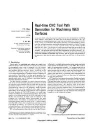
Figure R7.1-5 compares the molecular weight distribution for poly(hexamethylene 

adipamide) calculated from Flory’s most probable distribution6 

[Equation 

(R7.1-35)] for a conversion of 99% with the experimental values obtained 

by fractionation. One observes that the comparison is reasonably favorable. 

For termination by combination, the mole fraction of polymers with j 

repeating units is 

while the corresponding weight fraction is 

where p is given by Equation (R7.1-22) [i.e., p = B]. 

7.1.5 Anionic Polymerization 



To illustrate the development of the growth of live polymer chains with time, 

we will use anionic polymerization. In anionic polymerization, initiation takes 

place by the addition of an anion, which is formed by dissociation of strong 

bases such as hydroxides, alkyllithium, or alkoxides that react with the mono- 

mer to form an active center, . The dissociation of the initiator is very rapid 

and essentially at equilibrium. The propagation proceeds by the addition of 

monomer units to the end of the chain with the negative charge. Because the 

live ends of the polymer are negatively charged, termination can occur only by 

charge transfer to either the monomer or the solvent or by the addition of a 

6 

W j × 10 4 

P. J. Flory, 

1953). 

35 

30 

25 

20 

15 

10 

5 

0 

0 100 

MOL.WT. 

10,000 20,000 30,000 

p = 0.990 

j 

40,000 50,000 60,000 

200 300 400 500 

Figure 7-1 Molecular distribution. [Adapted from G. Tayler, Journal of the 

Fogler/Prenhall/F7.7 rev 12/11/97 

American Chemical Society, 69, p. 638, 1947. Reprinted by permission.] 

y j ( j � 1) 

( 1 � p) 

2 � 

p 

w j 

1 

2 

Principles of Polymer Chemistry, 

(Ithaca, N.Y.: Cornell University Press, 

j 2 � 

-- j ( 1 � p) 

3 � ( j � 1)p 

R 1 � 

j 2 �

Batch reactor 


neutralizing agent to the solution. Let 

for anionic polymerization becomes 

� and the sequence of reactions 

Initiation: 

Propagation: 

Chain transfer to solvent: 

Transfer to monomer: 

The corresponding combined batch reactor mole balances and rate laws are: 

For the initiator: 

For the live polymer: 

For the dead polymer: 

k 

i 

R j � R j 

AB ⎯⎯→ 

←⎯⎯ A � 

⎧ 

� B� 

k�i 

⎨ 

kp ⎩ A� 

� M ⎯⎯→ R 1 

⎧R1 

� M ⎯⎯→ R 2 

⎨ 

kp 

⎩R 

j� 

M ⎯⎯→ R j 

R j 

k 

In theory one could solve this coupled set of differential equations. However, 

this process is very tedious and almost insurmountable if one were to carry it 

through for molecular weights of tens of thousands of Daltons, even with the 

fastest of computers. Fortunately, for some polymerization reactions there is a 

way out of this dilemma. 

Some Approximations. To solve this set of coupled ODEs, we need to make 

some approximations. There are a number of approximations that could be 

made, but we are going to make ones that allow us to obtain solutions that provide 

insight on how the live polymerization chains grow and dead polymer 

k 

p 

�1 

tS 

�S ⎯⎯→ P j� 

S� 

calculations R j� M ⎯⎯→ P j� 

R1 

“Houston, we have a 

problem!” 

—Apollo 13 

k 

tm 

dA� ---------- � ki AB � k i 

dt 

� A�B� k p A� � M 

dR1 -------- k p A 

dt 

� n 

M�kpR1MktmM R � � 

� 

j � 1 

dRj 

-------- � k p ( R j� 

1 � R j)M�k 

dt 

tSSRj � ktmMRj dPj ------- � k 

dt 

tSSRj � ktmMRj j 

376

377 

Chap. 

chains form. First, we neglect the termination terms ( ktSSRj 

and ktmRj 

M) 

with 

respect to propagation terms in the mole balances. This assumption is an excellent 

one as long as the monomer concentration remains greater than the live 

polymer concentration. 

For this point, we can make several assumptions. We could assume that 

the initiator ( I � A�) 

reacts slowly to form R1 

(such is the case in Problem 

). 

CDP7-P 

B 

0 

I� M ⎯⎯→ R 1 

dR1 Initiation 

-------- � k0 MI � kp R 

dt 

1M 

Another assumption is that the rate of formation of R1 

from the initiator is 

instantaneous and that at time t � 0 the initial concentration of live polymer is 

R10 � I0. This assumption is very reasonable for this initiation mechanism. 

Under the latter assumption the mole balances become 

Propagation 

dR1 -------- � �k 

p MR1 dt 


dR2 -------- � k p MR ( 1�R2) dt 


… 

dRj -------- � k p ( R j� 1�R 

j)M 


dt 

For the live polymer with the largest chain length that will exist, the mole balance 

is 

dRn -------- � k p MRn� 1 

dt 

If we sum Equations (R7-1.38) through (R7-1.41), we find that 

dRj 

dt 

-------- 

n 

� dR� 

� -------- �0 

dt 

j � 1 


Consequently, we see the total free live polymer concentration is a constant at 

R * � R 10 � I 0. 

There are a number of different techniques that can be used to solve this 

set of equations, such as use of Laplace transforms, generating functions, statistical 

methods, and numerical and analytical techniques. We can obtain an 

analytical solution by using the following transformation. Let 

k 

d� � 

k p M dt 


Concentration of 

live polymer of 

chain length j 


Then Equation (R7.1-38) becomes 

dR1 -------- � �R1 

d� 

Using the initial conditions that when t � 0, then � � 0 and 

Equation (R7.1-43) solves to 

R1 I0 e � � � 

Next we transform Equation (R7.1-39) to 

and then substitute for 

R1: 

378 


R1 

� R10 

� I0,. 


With the aid of the integrating factor, e , along with the initial condition that 

at t � 0, � 0, � 0, we obtain 

� 

� 

R 

2 

In a similar fashion, 

In general, 

dR 2 

d� 

-------- � R1 � R2 dR2 -------- R2 d� 

� I0 e � � � 

R2 I0 �e � � � ( ) 

� 

R3 I0 2 

-------- e 

2�1 � � 

⎛ ⎞ 

� ⎜ ⎟ 

⎝ ⎠ 

� 

R4 I0 3 

--------------- e 

3�2�1 � � 

⎛ ⎞ 

� ⎜ ⎟ 

⎝ ⎠ 

R j 

� j 1 

I0 � 

----------------- e 

( j � 1)! 

� � 

� 


The live polymer concentrations are shown as a function of time and of chain 

length and time in Figures R7.1-6 and R7.1-7, respectively. 

Neglecting the rate of chain transfer to the monomer with respect to the 

rate of propagation, a mole balance on the monomer gives 

dM 

------- �k p M R 

dt � 

n 

k � 

� � MR � 

j � 1 

j 

p 

10 

�k 

p MI0 


Anionic 

polymerization 

Relationship 

between the scaled 

time, , and real 

time t 

379 

R j 

I 0 

R j 

I 0 

R 3 

Knowing the initial monomer concentration, 

mer concentration at any time: 

R 5 

Figure R7.1-6 Live polymer concentration as a function of scaled time. 

θ 3 

We can also evaluate the scaled time �: 

θ 5 

θ 

R 7 

Fogler/Prenhall/F7 8 

Figure R7.1-7 Live polymer concentration as a function of chain length at 

different scaled times. 

Fogler/Prenhall/F7.9 

M0 

t 

M M0e I0 kpt � 

� 

� � k p M d t � M � 

0 

j 

0 k p 

M 0 

� k p I 

------------ e 0 kpt 

k I 

� 

� ( ) 

� � M0 ------ 1 e 

I0 I0 kpt � 

� 

( � ) 

p 

0 

0 

t 

� 

t 

0 

e 

θ 7 

Chap. 

, we can solve for the mono- 

I0 

kpt 

� 

d t 




One can now substitute Equation (R7.1-48) into Equation (R7.1-45) to determine 

the live polymer concentrations at any time t. 

For anionic polymerization, termination can occur by neutralizing the 

live polymer to . 

R 

j 

P 

j 

Example R7–3 Calculating the Distribution Parameters from Analytical 

Expressions for Anionic Polymerization 

Calculate �n , �m , and D for the live polymer chains 

Solution 

R j I0 ----------------- e 

( j� 1)! 

We recall that the zero moment is just the total radical concentrations: 

� � 

� 

The first moment is 

Let k � j � 1: 

Expanding the ( k � 1) term gives 

Recall that 

Therefore, 

Let l � k � 1: 

� 

� 0 

� j�1 

� 

R � j 

j�1 

�1 jR � j I 

� � 

j�1 

� � I0 0 

� 

� 

j�1 

Rj. 

j� 

j�1e�� 

----------------------- 

( j � 1 ) ! 

� �ke�� 

�1 � I0 ( k �1) 

--------------- 

� k! 

k�0 

�1 I0 � ke�� 

k � k 

--------------k 

! 

e 

⎛ � 

� ��⎞ 

� ⎜ � ------------------ 

⎝��⎟ k ! ⎠ 

k�0 

� 

� 

k�0 

k�0 

� k 

k ! 

----- e �� 

�1 I0 1 e � � k � k 

k ! 

-------- 

⎛ � ⎞ 

� 

⎜ � 

⎝ � ⎟ 

⎠ 

k�0 

380 

( R7.1-45) 

(RE7-3.1) 

(RE7-3.2) 

(RE7-3.3) 

(RE7-3.4) 

(RE7-3.5) 

(RE7-3.6)

381 

The first moment is 

�1 I0 1 e � � � � l 

l ! 

----- 

⎛ � ⎞ 

� ⎜ � 

⎝ � ⎟ � I 0 ( 1� 

e��e�) 

⎠ 

l�0 

�1 � I0 ( 1� �) 

The number-average length of growing polymer radical (i.e., live polymer) is 

� n 

� 

j�0 

�1 �0 � ---- �1�� 

2 � j�1 

�2 I0 j 2 � R � j � I0 

j ----------------- 

� ( j � 1) 

! 

Chap. 

(RE7-3.7) 

(RE7-3.8) 

(RE7-3.9) 

(RE7-3.10) 

Realizing that the j � 0 term in the summation is zero and after changing the index 

of the summation and some manipulation, we obtain 

(RE7-3.11) 

(RE7-3.12) 

(RE7-3.13) 

Plots of �n and �w along with the polydispersity, D, 

are shown in Figure RE7-3.1. 

We note from Equation (R7.1-48) that after a long time the maximum value 

of �, �M , will be reached: 

The distributions of live polymer species for an anionic polymerization carried out 

in a CSTR are developed in Problem P7-19. 

Example R7–4 Determination of Dead Polymer Distribution When Transfer 

to Monomer Is the Main Termination Mechanism 

Determine an equation for the concentration of polymer as a function of scaled 

time. After we have the live polymer concentration as a function of time, we can 

determine the dead polymer concentration as a function of time. If transfer to monomer 

is the main mechanism for termination, 

� 

j�0 

�2 I0 1 3� �2 � ( � � ) 

� w 

�2 ---- 

�1 1 3� �2 � � 

� � ----------------------------- 

1� � 

D �w 1 3� � 

----- 

2 � � 

( 1� �) 

2 

� � ----------------------------- 

R j 

� n 

� M 

M0 � ------ 

I0 k 

tm 

�M ⎯⎯→ P j� 

R1

Anionic 

polymerization 


µ N 

1.0 1.0 

µ D 

θ 

(a) 

1.0 

Figure RE7-3.1 Moments of live polymer chain lengths: (a) number-average chain 

Fogler/Prenhall/E7.5.1 

length; (b) weight-average chain length; (c) polydispersity. 

A balance of dead polymer of chain length j is 

382 

dPj ------- � ktm R j M 

(RE7-4.1) 

dt 

As a very first approximation, we neglect the rate of transfer to dead polymer from 

the live polymer with respect to the rate of propagation: 

so that the analytical solution obtained in Equation (R7.1-4.2) can be used. Then 

dPj -----d� 

(RE7-4.2) 

Integrating, we obtain the dead polymer concentrations as a function of scaled time 

from CRC Mathematical Tables integral number 521: 

We recall that the scaled time � can be calculated from 

µ w 

θ 

(c) 

( ktm MRj �k 

p MRj) ktm 

I 0 � j�1e�� 

� ------ R j � ------ -------------------------- 

( j � 1) 

! 

ktm k p 

ktm � ------ I 0 1� 

e 

k p 

�� 

k 

p 

j�1 

� 

?0l? �0 

� M0 ------ 1 e 

I0 I0 kpt � 

� 

( � ) 

�( 

j�1�?0l? 

) 

---------------------------------- 

( j� 

1 � ?0l? ) ! 

θ 

(b) 

(RE7-4.3)

383 

Chap. 

In many instances termination of anionic polymerization is brought about by adding 

a base to neutralize the propagating end of the polymer chain. 

Other Useful Definitions. The number-average kinetic chain length, VN, 

is 

the ratio of the rate of the propagation rate to the rate of termination: 

r p 

V N � ---- 


rt Most often, the PSSH is used so that rt 

� ri: 

r p 

V N � ---ri 

The long-chain approximation holds when VN 

is large. 

Excellent examples that will reinforce and expand the principles discussed 

in this section can be found in Holland and Anthony, 7 and the reader is 

encouraged to consult this text as the next step in studying polymer reaction 

engineering. 

For the free-radical polymerization in which termination is by transfer to 

the monomer or a chain transfer agent and by addition, the kinetic chain length is 

For termination by combination 

Mn � 2V N MM and for termination by disproportionation 

7 

V N 

r p 

--rt 

k p MR� ktmMR� kt R� ( ) 2 kCt R� ------------------------------------------------------------------ 

� � C 

k p M 

� � � ---------------------------------------------- 

V N 

k p M 

ktmM ( 2kt koI 2 f ) 12 / � ------------------------------------------------------------------- 

� �kctC 

Mn � 

V N MM ktmM ktR� � �kctC 

(R7-1.50) 

C. D. Holland and R. G. Anthony, Fundamentals of Chemical Reaction Engineering, 

2nd ed. (Upper Saddle River, N.J.: Prentice Hall, 1977) p. 457.

R7.1 Polymerization

Create successful ePaper yourself

Delete template?

Save as template?