Modeling and Calibration of a Structured-light Optical - Michigan ...
Modeling and Calibration of a Structured-light Optical - Michigan ...
Modeling and Calibration of a Structured-light Optical - Michigan ...

Create successful ePaper yourself
Turn your PDF publications into a flip-book with our unique Google optimized e-Paper software.
Chenggang Che<br />
Graduate Research Assistant.<br />
Jun Ni<br />
Associate Pr<strong>of</strong>essor.<br />
Department <strong>of</strong> Mechanical Engineering<br />
<strong>and</strong> Applied Mechanics,<br />
The University <strong>of</strong> <strong>Michigan</strong>,<br />
Ann Arbor, Ml 48109<br />
1 Introduction<br />
The accurate measurement, or digitization <strong>of</strong> free-form surfaces<br />
<strong>and</strong> parts with complex features, such as dies <strong>and</strong> molds,<br />
ship hulls, airplane fuselages, wings <strong>and</strong> turbine blades, etc.,<br />
has always been a tedious <strong>and</strong> time consuming task. Although<br />
designers <strong>of</strong>ten specify a tight control tolerance over the entire<br />
three dimensional contour surface, manufacturers <strong>and</strong>/or inspectors<br />
have difficulty employing a rigorous method to measure<br />
<strong>and</strong> check the entire surface. The most popular measurement<br />
tools used to perform sampled measurement <strong>of</strong> these surfaces<br />
are Coordinate Measurement Machines (CMMs) using<br />
contact probes. These devices, while having more than sufficient<br />
measurement accuracy for the defined task, suffer from the<br />
relatively low measurement throughput which makes the measurement<br />
task time consuming.<br />
To address this problem, a number <strong>of</strong> vendors <strong>and</strong> researchers<br />
have developed non-contact laser probes for digitizing surfaces<br />
by employing a single-spot beam to sweep the entire surface<br />
to be measured (Aromat, 1992; Keyence, 1993; Okada, 1992;<br />
Selcom, 1993; Venture, 1993; CyberOptics, 1992; Hymarc,<br />
1994; Chesapeake Laser, 1994; Digibotics, 1994; Goh, et al.,<br />
1985; Saito <strong>and</strong> Miyoshi, 1991; Bradley <strong>and</strong> Vickers, 1992,<br />
etc.). These devices, while faster than their contact probe equivalents,<br />
suffer similar throughput limitations <strong>and</strong> <strong>of</strong>ten have difficulty<br />
locating certain features accurately, particularly edges &<br />
holes. Thus, the development <strong>of</strong> high-throughput dimensional<br />
measurement/digitization techniques for large <strong>and</strong> complex<br />
free-form surfaces becomes necessary.<br />
With the emergence <strong>of</strong> large field <strong>of</strong> view structured-<strong>light</strong><br />
laser stripe sensors in recent years (Perceptron, 1994ab; Sami,<br />
1994; Geometric Research, 1994; 3D Technology, 1994, etc.),<br />
integration <strong>of</strong> such 2D contour sensors to multiple-axis machines<br />
such as CNC, CMM or robot systems has generated some<br />
interests (Chen, 1991; Champ, 1992). Chen (1991) studied the<br />
case <strong>of</strong> single axis scanning.<br />
Some earlier work was done by Will <strong>and</strong> Pennington (1971,<br />
1972), Popplestone et al. (1975), Agin <strong>and</strong> Binford (1973),<br />
Agin <strong>and</strong> Highnam (1982), Agin (1985) <strong>and</strong> Mansbach<br />
(1986). Their modeling methodologies were all based on a pinhole<br />
camera model. Their calibration approaches required the<br />
measurement <strong>of</strong> both camera/projector parameters <strong>and</strong> robot<br />
joint parameters, thus making on-line use impossible.<br />
Contributed by the Manufacturing Engineering Division for publication in die<br />
JOURNAL OF MANUFACTURING SCIENCE AND ENGINEERING. Manuscript received<br />
Jan. 1995; revised Aug. 1995. Technical Editor: S. K. Kapoor.<br />
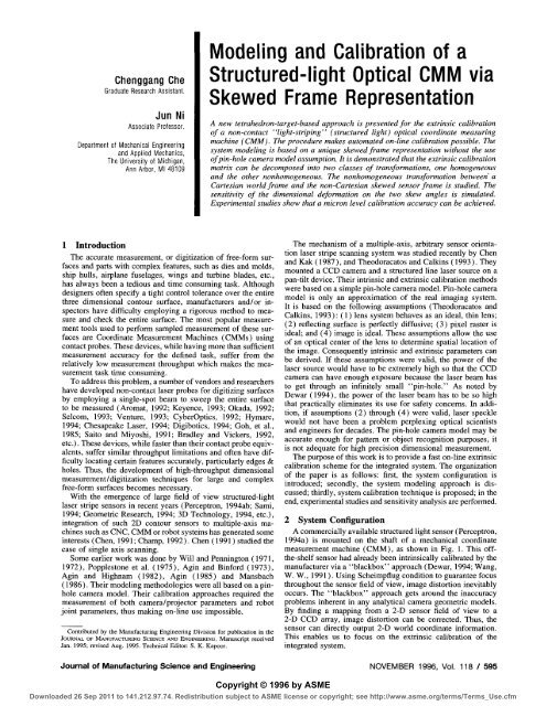
<strong>Modeling</strong> <strong>and</strong> <strong>Calibration</strong> <strong>of</strong> a<br />
<strong>Structured</strong>-<strong>light</strong> <strong>Optical</strong> CMM via<br />
Skewed Frame Representation<br />
A new tetrahedron-target-based approach is presented for the extrinsic calibration<br />
<strong>of</strong> a non-contact "<strong>light</strong>-striping" (structured <strong>light</strong>) optical coordinate measuring<br />
machine (CMM). The procedure makes automated on-line calibration possible. The<br />
system modeling is based on a unique skewed frame representation without the use<br />
<strong>of</strong> pin-hole camera model assumption. It is demonstrated that the extrinsic calibration<br />
matrix can be decomposed into two classes <strong>of</strong> transformations, one homogeneous<br />
<strong>and</strong> the other nonhomogeneous. The nonhomogeneous transformation between a<br />
Cartesian world frame <strong>and</strong> the non-Cartesian skewed sensor frame is studied. The<br />
sensitivity <strong>of</strong> the dimensional deformation on the two skew angles is simulated.<br />
Experimental studies show that a micron level calibration accuracy can be achieved.<br />
The mechanism <strong>of</strong> a multiple-axis, arbitrary sensor orientation<br />
laser stripe scanning system was studied recently by Chen<br />
<strong>and</strong> Kak (1987), <strong>and</strong> Theodoracatos <strong>and</strong> Calkins (1993). They<br />
mounted a CCD camera <strong>and</strong> a structured line laser source on a<br />
pan-tilt device. Their intrinsic <strong>and</strong> extrinsic calibration methods<br />
were based on a simple pin-hole camera model. Pin-hole camera<br />
model is only an approximation <strong>of</strong> the real imaging system.<br />
It is based on the following assumptions (Theodoracatos <strong>and</strong><br />
Calkins, 1993): (1) lens system behaves as an ideal, thin lens;<br />
(2) reflecting surface is perfectly diffusive; (3) pixel raster is<br />
ideal; <strong>and</strong> (4) image is ideal. These assumptions allow the use<br />
<strong>of</strong> an optical center <strong>of</strong> the lens to determine spatial location <strong>of</strong><br />
the image. Consequently intrinsic <strong>and</strong> extrinsic parameters can<br />
be derived. If these assumptions were valid, the power <strong>of</strong> the<br />
laser source would have to be extremely high so that the CCD<br />
camera can have enough exposure because the laser beam has<br />
to get through an infinitely small "pin-hole." As noted by<br />
Dewar (1994), the power <strong>of</strong> the laser beam has to be so high<br />
that practically eliminates its use for safety concerns. In addition,<br />
if assumptions (2) through (4) were valid, laser speckle<br />
would not have been a problem perplexing optical scientists<br />
<strong>and</strong> engineers for decades. The pin-hole camera model may be<br />
accurate enough for pattern or object recognition purposes, it<br />
is not adequate for high precision dimensional measurement.<br />
The purpose <strong>of</strong> this work is to provide a fast on-line extrinsic<br />
calibration scheme for the integrated system. The organization<br />
<strong>of</strong> the paper is as follows: first, the system configuration is<br />
introduced; secondly, the system modeling approach is discussed;<br />
thirdly, system calibration technique is proposed; in the<br />
end, experimental studies <strong>and</strong> sensitivity analysis are performed.<br />
2 System Configuration<br />
A commercially available structured <strong>light</strong> sensor (Perceptron,<br />
1994a) is mounted on the shaft <strong>of</strong> a mechanical coordinate<br />
measurement machine (CMM), as shown in Fig. 1. This <strong>of</strong>fthe-shelf<br />
sensor had already been intrinsically calibrated by the<br />
manufacturer via a "blackbox" approach (Dewar, 1994; Wang,<br />
W. W., 1991). Using Scheimpflug condition to guarantee focus<br />
throughout the sensor field <strong>of</strong> view, image distortion inevitably<br />
occurs. The "blackbox" approach gets around the inaccuracy<br />
problems inherent in any analytical camera geometric models.<br />
By finding a mapping from a 2-D sensor field <strong>of</strong> view to a<br />
2-D CCD array, image distortion can be corrected. Thus, the<br />
sensor can directly output 2-D world coordinate information.<br />
This enables us to focus on the extrinsic calibration <strong>of</strong> the<br />
integrated system.<br />
Journal <strong>of</strong> Manufacturing Science <strong>and</strong> Engineering NOVEMBER 1996, Vol. 118/595<br />
Copyright © 1996 by ASME<br />
Downloaded 26 Sep 2011 to 141.212.97.74. Redistribution subject to ASME license or copyright; see http://www.asme.org/terms/Terms_Use.cfm
Fig. 1 Integration <strong>of</strong> a laser stripe sensor to a CMM<br />
The multiple-axis integrated system allows the sensor to be<br />
rotated to any angle for optimal view <strong>of</strong> the part surface to be<br />
measured. The same sensor can also be attached to the endeffector<br />
<strong>of</strong> a robot. The robot itself cannot be used for scanning<br />
due to its poor positioning accuracy. However, when combined<br />
with a precision X-Y motion stage, the robot integrated system<br />
has its advantages: the robot arm can easily position the sensor<br />
to reach <strong>and</strong> measure large parts from many positions <strong>and</strong> orientations.<br />
Since the laser scanner is only a two dimensional sensor, a<br />
third dimension needs to be integrated to the system to realize<br />
3-D measurements. When scanning a part, the CMM shaft<br />
moves the sensor along a certain axis, e.g., the X axis, in small<br />
increments at a fixed speed. The sensor provides Ys <strong>and</strong> Zs data<br />
while the optical (or magnetic) scale <strong>of</strong> the CMM X axis provides<br />
the Xs information (Fig. 2). If the part instead <strong>of</strong> the<br />
sensor moves, the scanning mechanism is the same.<br />
If the laser plane, on which the sensor coordinate frame Ys-<br />
Zs lies, is always perpendicular to the surface to be measured<br />
(i.e., the laser plane is placed perpendicular to the CMM Xaxis),<br />
the coordinate system thus formed is Cartesian. However,<br />
this severely limits the application <strong>of</strong> the system, practically<br />
precluding the measurement <strong>of</strong> complex parts requiring multiple-axis<br />
scanner motions <strong>and</strong> multiple orientations <strong>of</strong> the laser<br />
sensor to achieve an optimal projecting angle.<br />
During scanning, the laser scanning coordinate system usually<br />
is non-orthogonal, i.e., skewed. If data obtained from this<br />
mechanical driving<br />
direction(Xs)<br />
<strong>Structured</strong> laser<br />
line <strong>light</strong>ing<br />
/ Sensing optics<br />
>• Xs: added axis<br />
Fig. 2 2D sensor used for 3D measurement<br />
596 / Vol. 118, NOVEMBER 1996<br />
imaginary Cartesian sensor Zs(Zs')<br />
coordinate system {S'}<br />
world coordinate system {W}<br />
Xw<br />
YsCYs 1 )<br />
real skewed sensor<br />
coordinate system (S}<br />
Fig. 3 Characterization <strong>of</strong> the laser stripe scanning system<br />
skewed coordinate system are to be used for dimensional measurement,<br />
they have to be transformed to a Cartesian frame.<br />
Otherwise, the dimensions on the part will be distorted, e.g.,<br />
after non-Cartesian scanning, a sphere in real space will look<br />
like an ellipsoid <strong>and</strong> a cube will look like an inclined parallelepiped.<br />
3 System <strong>Modeling</strong><br />
3.1 Skewed Frame Representation. Three frames, the<br />
world coordinate frame {W}, an imaginary sensor coordinate<br />
system {S'} <strong>and</strong> the sensor's body frame {S}, as shown in<br />
Figs. 3 <strong>and</strong> 4, are used in the following discussions. Both {W}<br />
<strong>and</strong> {S'} are Cartesian frames, but {S} frame is not. {S} <strong>and</strong><br />
{S'} frames share the same origin. Let b aTbe the 4 X 4 matrix<br />
representation <strong>of</strong> coordinate transformation from {a} to {b},<br />
a, b e {W,S',S). Then<br />
T is a homogeneous transform <strong>of</strong> which various equivalent<br />
representations exist (e.g., Craig, 1992; Wang, 1992). This paper<br />
adopts the matrix representation using the roll-pitch-yaw<br />
angles (a, /3, y):<br />
"T =<br />
cacfi<br />
sac (3<br />
-sp<br />
0<br />
cas0sy — sacy<br />
sasfisy + cacy<br />
cfisy<br />
0<br />
caspcy + sasy<br />
sas/3cy — easy<br />
c0cy<br />
0<br />
: where sin a sa, cos a •• = COL <strong>and</strong> (qx,qy,qz, 1 )<br />
vector Neither fT nor<br />
form. Their representations are explored below<br />
T is a translation<br />
W<br />
T constitutes a homogeneous trans-<br />
Ys(Ys<br />
A x^<br />
Fig. 4 Spatial relationship between the real skewed sensor coordinate<br />
system {S} <strong>and</strong> the imaginary Cartesian coordinate system {S }<br />
(1)<br />
(2)<br />
Transactions <strong>of</strong> the ASME<br />
Downloaded 26 Sep 2011 to 141.212.97.74. Redistribution subject to ASME license or copyright; see http://www.asme.org/terms/Terms_Use.cfm
In Figs. 3 <strong>and</strong> 4, the orientation <strong>of</strong> the real sensor Xs axis in<br />
the imaginary Cartesian sensor coordinate system {S'} can be<br />
defined by two angles, 9 <strong>and</strong> ip. 9 is defined as the angle between<br />
axes Xs <strong>and</strong> Xs'. ip is defined as the angle between Xprj (the<br />
orthogonal projection <strong>of</strong> Xs axis onto the Ys-ZslYs'-Zs' plane)<br />
<strong>and</strong> Ys.<br />
Point P is used to find the transformation from {S} to {S'}.<br />
P has two sets <strong>of</strong> coordinates, {x, y, z) in {S} <strong>and</strong> (x', y', z')<br />
m{S'}.<br />
Since the laser plane [Ys - Zs] moves along the Xs axis<br />
during scanning, the (x, y, z) coordinates <strong>of</strong> P in sensor frame<br />
are not all perpendicular projections onto the three axes <strong>of</strong> {S}.<br />
P' is the intersection <strong>of</strong> line PP' <strong>and</strong> the Ys-Zs plane, <strong>and</strong> PP'<br />
the second or the third column <strong>of</strong> the corresponding transformation<br />
matrices <strong>of</strong> Eq. (4) <strong>and</strong> Eq. (6).<br />
From Eq. (6), when 9 = 0°, fTbecomes an identical matrix.<br />
This implies that no skew transformations are involved, which<br />
is intuitively correct. When the Xs' axis coincides with the Xs<br />
axis, i.e., when the mechanical driving system is perpendicular<br />
to the 2D sensor plane, the coordinate system will become<br />
orthogonal. Here we limit the parameters to 0 deg s 9 < 90<br />
deg <strong>and</strong> 0 deg s \p =s 360 deg. We have no interest in 180 deg<br />
a 6 a 90 deg because the coordinate frame will be left-h<strong>and</strong>ed.<br />
Combining the nonhomogeneous coordinate transformation<br />
matrix f'T<strong>and</strong> the homogeneous coordinate transformation matrix<br />
y T, the composition gives<br />
cached + (casfisy — sacy)s9cip + (casficy + sasy)s9stp caspsy — sacy casficy + sasy qx<br />
sac0c9 + (sasfisy + cacy)s9cip + (sas/3cy — casy)s9sip sasPsy + cacy sasficy — easy qy<br />
-sficO + c{3sys9cip + cficys8sip cfisy cficy qz<br />
is parallel to axis Xs. The y <strong>and</strong> z coordinates <strong>of</strong> P, which<br />
are the lengths <strong>of</strong> OB <strong>and</strong> OA, are formed by the perpendicular<br />
projections <strong>of</strong> P' onto the Ys (Ys') <strong>and</strong> Zs (Zs') axes,<br />
respectively. Coordinate x <strong>of</strong> P is formed by a parallel projection<br />
<strong>of</strong> P onto Xs axis. The line <strong>of</strong> parallel projection PC is parallel<br />
to OP'. Thus, the x coordinate <strong>of</strong> P is formed by a parallel<br />
projection while the y <strong>and</strong> z coordinates are formed by perpendicular<br />
projections. This characteristic is very different from<br />
that <strong>of</strong> a normal Cartesian coordinate system, where all the<br />
point coordinates are formed by perpendicular projections.<br />
To derive the transformation between the two frames, the<br />
algebraic relationship between (x, y, z) <strong>and</strong> (x', y', z') needs<br />
to be established. We have,<br />
or in matrix form,<br />
s T -<br />
X = x' • sec 9<br />
• y = y' — x' -tan 9 -cos ip<br />
. z = z' - x' -tan #-sin ip<br />
|~ sec 9 0 0 0 1<br />
-tan 9 cos tp 1 0 0<br />
-tan 9 sin ip 0 1 0<br />
0 0 0 1 J<br />
Note that S S>T\s non-orthonormal. Besides, it is undefined at<br />
9 = 90 deg which disables the data collection.<br />
From Eq. (3), the inverse transformation | Teem be obtained<br />
as<br />
or in matrix form<br />
x = x • cos 9<br />
y' = y + x • sin 9 cos \p<br />
z' = z + x• sin 9 sin ip<br />
• cos 9 0 0 0'<br />
sin 8 cos ip 1 0 0<br />
sin 9 sin ip 0 1 0<br />
0 0 0 1<br />
Note that both f. T <strong>and</strong> f' T are non-orthonormal. If the Ys or<br />
Zs axis were skewed, non-orthogonal terms would appear in<br />
0 0 0 1<br />
(3)<br />
(4)<br />
(5)<br />
(6)<br />
which describes the entire laser stripe scanning process.<br />
3.2 Properties <strong>of</strong> the Composition Matrix <strong>and</strong> Identification<br />
<strong>of</strong> Extrinsic Parameters. When the angular encoder<br />
<strong>of</strong> the pan-tilt device is accurate enough, external calibration<br />
needs to be done only once when the system is initially setup.<br />
All the rest <strong>of</strong> the external re-calibrations could be avoided by<br />
knowing all the parameters <strong>of</strong> the position <strong>and</strong> orientation <strong>of</strong><br />
the sensor. However, if the accuracy <strong>of</strong> the angular encoder is<br />
not good enough, the calibration matrix <strong>of</strong> (7) has to be identified<br />
whenever a change in sensor position or orientation occurs.<br />
In this section, the properties <strong>of</strong> the calibration matrix are explored<br />
<strong>and</strong> extrinsic parameters are derived to facilitate onetime<br />
calibration when system angular encoder is accurate.<br />
Since the three projections <strong>of</strong> the skewed sensor coordinate<br />
system are not all perpendicular projections, six parameters<br />
which are usually required <strong>of</strong> any homogeneous coordinate<br />
transformation can not fully describe the skewed frame transformation<br />
here. Two extra parameters, 9 <strong>and</strong> ip, are needed. Therefore,<br />
the number <strong>of</strong> extrinsic parameters extends to eight: five<br />
angular parameters {a, (3, y, 9, tp] <strong>and</strong> three translational parameters<br />
{qx, qy, qz].<br />
We can also write the overall transformation as<br />
tn fl2 fl3 Pi<br />
til hi ?23 Pi<br />
hx hi ?33 P3<br />
0 0 0 1<br />
" R p~<br />
0 1<br />
where R is a composition <strong>of</strong> rotation, shearing <strong>and</strong> scaling transformations<br />
<strong>and</strong> P = (pi, p2, PT, ) T is the translational vector. The<br />
orthonormality <strong>of</strong> a matrix governs that the norms <strong>of</strong> its three<br />
column vectors are one <strong>and</strong> that the three cross products <strong>of</strong> the<br />
vectors are zero, which gives six constraints to twelve variables.<br />
For the multiple-axis laser scanning process, due to the introduction<br />
<strong>of</strong> a skewed axis, two <strong>of</strong> the three orthogonality constraints<br />
are relaxed <strong>and</strong> it can be shown that the following four constraints<br />
exist for the overall transformation fT,<br />
Journal <strong>of</strong> Manufacturing Science <strong>and</strong> Engineering NOVEMBER 1996, Vol. 118/597<br />
Downloaded 26 Sep 2011 to 141.212.97.74. Redistribution subject to ASME license or copyright; see http://www.asme.org/terms/Terms_Use.cfm<br />
(7)<br />
(8)<br />
(9)
tu + ?2i + hi<br />
t\2 + ?22 + ^32<br />
'l3 1" J 23 T" '33<br />
?12'?13 + ^22'?23 + ?32 ''33 = 0<br />
(10)<br />
<strong>of</strong> which the top three are normality constraints <strong>and</strong> the fourth<br />
one is an orthogonality constraint (governs the orthogonality<br />
<strong>of</strong> the sensor Ys <strong>and</strong> Zs axis). We can also write Eq. (10) in<br />
matrix form,<br />
where<br />
R T -R =<br />
1 K\ K2<br />
K, 1 0<br />
K2 0 1<br />
" 1 — ?llf 12 + ^21^22 "t~ ^31^32<br />
K2 = fll^l3 + ^21^23 + ?31^33<br />
(ID<br />
(12)<br />
^ is the inner product <strong>of</strong> the first <strong>and</strong> second column vectors<br />
<strong>of</strong> the transformation matrix fT, thus represents the non-orthogonality<br />
<strong>of</strong> the sensor Xs axis <strong>and</strong> Ys axis. K2 is the inner product<br />
<strong>of</strong> the first <strong>and</strong> third column vectors <strong>of</strong> JT, thus represents the<br />
non-orthogonality <strong>of</strong> the sensor Xs axis <strong>and</strong> Zs axis. It can be<br />
shown that the two skew angles are uniquely determined by Ki<br />
<strong>and</strong> K2,<br />
ip = tan \K2IKX)<br />
= sin ' (VK? + /c|)<br />
(13)<br />
Were the coordinate systems orthogonal, the transformation<br />
matrix f T would have been orthonormal, which means that we<br />
should have had R T -R = /. When T is orthonormal, «i <strong>and</strong><br />
K2 approach zero <strong>and</strong> 9 becomes zero. This makes sense because<br />
6 is the skew angle <strong>of</strong> Xs axis. In the meantime, ip turns undefined,<br />
which is also true when the definition <strong>of</strong> ip is referred in<br />
Figure 4.<br />
To solve for the initial extrinsic parameters <strong>of</strong> the system,<br />
equate the corresponding terms <strong>of</strong> matrix fT in Eqs. (7) <strong>and</strong><br />
(8), twelve equations are found. Solving the 12 simultaneous<br />
equations, we have<br />
aa = tan" 1 [(tl3t32 - t^h^lih^ - t23tn)]<br />
(30 = cos" 1 Mi + '33<br />
, y„ = tair'tez/fss)<br />
(14)<br />
Subsequent angular motions <strong>of</strong> the pan-tilt device can be measured<br />
by the angular encoder as Aa, A/?, Ay. Then the current<br />
roll-pitch-yaw angles become a = a0 + Aa, p = /3a + A/3, y<br />
= yD + Ay. Knowing these angles, a new transformation matrix<br />
can be readily calculated from (7), thus saving subsequent<br />
calibrations.<br />
4 Sensitivity Analysis <strong>of</strong> Dimensional Deformation<br />
The nonhomogeneous coordinate transformation <strong>of</strong> the laser<br />
scanning process is not a shape <strong>and</strong> dimension preserving transformation.<br />
In this section, sensitivity analysis <strong>of</strong> deformation<br />
due to the two skew angles are performed by computer simulation.<br />
4.1 Euclidean Length Deformation. Given two arbitrary<br />
points P,(x[, y\, z[) <strong>and</strong> P2(^2, yk, Z2) in a 3D Cartesian<br />
space, e.g., the imaginary Cartesian sensor frame {S'}, it is <strong>of</strong><br />
interest to know how the distance between the two changes<br />
after the nonhomogeneous coordinate transformation. The coordinates<br />
<strong>of</strong> the same two points in the true skewed sensor frame<br />
598 / Vol. 118, NOVEMBER 1996<br />
{S} can be calculated from Eq. (3) as Pi (xt, yx, Z\) <strong>and</strong> P2 (x2,<br />
y2,z2). If the distance between the two points in Cartesian space<br />
is d\2, after the transformation <strong>of</strong> Eq. (4), the length deformation<br />
is<br />
where<br />
Adn(6, i},) = U\l + Dl2(d, i//) - d[2<br />
Dn(0,
Fig. 6 Angular deformation as a function <strong>of</strong> the skew angles<br />
Aa(9, i/0 = cos" 1 ,<br />
U\l + D12 Ull + D<br />
where<br />
-cos"' (19)<br />
d[2-d[3<br />
AC = -tan #-(cos t/j-(dx[2 • dy'n + dx'n • dy[2)<br />
D,2 = 2 tan 0- dx[2 (tan 9- dx',2<br />
+ sin tp-{dx\2 • dz[3 + dx'n • dz[2))<br />
\ — cos t/j- dy'l2 — sin if/ • dz \2)<br />
Dn = 2 tan 0-dx[3 (tan 9- dx'n<br />
— cos (//• dy[3 — sin iff- dz'n)<br />
. C = dx[2 • dx'n + dy[2 • dy'n + dz[2' dz'n (20)<br />
The percentage error <strong>of</strong> angular deformation Ea as a function<br />
<strong>of</strong> the two skew angles is shown in Fig. 6. When 9 increases,<br />
the angular deformation does not always increase. Indeed it<br />
looks like a "saddle." The "saddle" <strong>of</strong> angular deformation<br />
in Fig. 6 is greater than that <strong>of</strong> length deformation in Fig. 5.<br />
Aside from the "saddle" effect, angular deformation increases<br />
almost linearly with the increase <strong>of</strong> 9. Although the<br />
deformations do depend on different selections <strong>of</strong> coordinate<br />
systems, the overall shape, i.e., the characteristics <strong>of</strong> the deformation<br />
surface does not change.<br />
4.3 Computer Simulation <strong>of</strong> Shape Deformation. Unlike<br />
length <strong>and</strong> angular deformation analysis, shape deformation<br />
analysis cannot proceed in an explicit way due to difficulties<br />
<strong>of</strong> shape representation. Instead, an example <strong>of</strong> sphere deformation<br />
is presented by computer simulation. Take a computer generated<br />
spherical surface <strong>and</strong> map all the points on the surface<br />
from a 3D Cartesian space to a skewed non-Cartesian space,<br />
we want to know how the shape <strong>of</strong> the sphere changes by<br />
observing the changes in radius <strong>and</strong> center locations. For a better<br />
observation <strong>of</strong> center location changes, two sphere surfaces are<br />
generated so that the distance between the centers <strong>of</strong> the two<br />
spheres reflects the changes in center locations.<br />
The mapping <strong>of</strong> data from a Cartesian space to a skewed<br />
non-Cartesian space is done by multiplying matrix f. T to all<br />
the spherical surface points. The deformations <strong>of</strong> radius <strong>and</strong><br />
center distance are again represented in a percentage error form.<br />
The angles 9 <strong>and</strong> ip range from 5 deg to 80 deg. As can be seen<br />
Fig. 7 Sensitivity <strong>of</strong> shape deformation reflected by radius change<br />
Fig. 8 Sensitivity <strong>of</strong> shape deformation reflected by distance change<br />
between centroids <strong>of</strong> two spheres<br />
from Figs. 7 <strong>and</strong> 8, both the radius <strong>and</strong> distance deformations<br />
are smoother than that <strong>of</strong> length <strong>and</strong> angle deformations <strong>of</strong> Figs.<br />
5 <strong>and</strong> 6. Also, the maximum changes <strong>of</strong> radius (up to 140 times<br />
larger than original radius) <strong>and</strong> distance (up to 25 times larger<br />
than original distance) are much larger than that <strong>of</strong> length (only<br />
5 times larger than original length) <strong>and</strong> angular (only 12 times<br />
larger than original angle) deformations. This is due to the fact<br />
that sec 9 <strong>and</strong> tan 9 terms in S s-T <strong>of</strong> Eq. (4) go to infinity when<br />
9 approaches 90 deg. The radius deformation surface in Fig. 7<br />
has the same pattern as the distance deformation surface in Fig.<br />
8. When 9 is fixed, both deformations almost linearly increase<br />
with the increase <strong>of</strong> tp. When ip is fixed, both deformations<br />
increase nearly exponentially with increase <strong>of</strong> 9. This agrees<br />
with our previous conclusion that 9 has more influence than
Given a commercial laser stripe sensor, it is not only unnecessary<br />
but also impossible to perform intrinsic calibration. Therefore<br />
it is impossible to combine the intrinsic <strong>and</strong> extrinsic calibration.<br />
The sensor frame is regarded as stationary instead <strong>of</strong> moving<br />
when skewed frame representation is employed. The advantage<br />
<strong>of</strong> this modeling is that scan data can be pooled as they are<br />
collected, i.e., no postprocessing <strong>of</strong> the data is necessary before<br />
performing extrinsic calibration. This makes it possible to scan<br />
a target in the sensor field <strong>of</strong> view <strong>and</strong> extract desirable feature<br />
points directly from the scanned data for extrinsic calibration.<br />
The use <strong>of</strong> moving frame model prevented Chen <strong>and</strong> Kak<br />
(1987) from knowing where exactly the object points are located<br />
so that they had to scan at least six non-parallel lines on a<br />
polyhedron target for calibration. We present a new tetrahedrontarget-based<br />
extrinsic calibration approach without the use <strong>of</strong><br />
pin-hole assumption. Two scan lines are all that are needed to<br />
calculate the four conjugate pairs, <strong>and</strong> the two lines can be<br />
parallel. The new calibration procedure becomes so simple that<br />
frequent on-line calibration becomes feasible whenever the system<br />
configuration is altered.<br />
5.1 <strong>Calibration</strong> Algorithm Formulation. The same<br />
point Pt in a 3D Euclidean space can be represented by two<br />
sets <strong>of</strong> coordinate vectors, one in the non-Cartesian skewed<br />
sensor frame, Psi = (xsi, ysi, zst) T <strong>and</strong> the other in the Cartesian<br />
world frame, Pwi = (xni,ywi, zwd T • These two coordinate vectors<br />
are <strong>of</strong>ten called "conjugate pairs" because they describe the<br />
same point in two different coordinate systems. For extrinsic<br />
calibration, we need to find the matrix JT from n conjugate<br />
pairs. Then the absolute orientation solution becomes a constrained<br />
least squares optimization problem (Che, 1995). That<br />
is, we want to minimize the augmented objective function<br />
F = I HP* - JT-Psi || 2 + \,[r?, + t 2 2l + t 2 M - 1]<br />
i=l<br />
+ X2-+[f?2 + t\2 + t\2 " 1] + \3[t\3 + th + tj3 - 1]<br />
t22' in + h2' hi ] (21)<br />
where the \,'s are Lagrange multipliers. Since there are four<br />
constraints among the twelve unknowns <strong>of</strong> T, only eight independent<br />
parameters exist. Therefore a minimum <strong>of</strong> three conjugate<br />
pairs are needed as they provide nine coordinates.<br />
However, this makes the algorithm nonlinear. For on-line<br />
use, a linear algorithm has to be found to provide an initial<br />
guess to the nonlinear algorithm. This is achieved by ignoring<br />
the four constraints in Eq. (21). The objective function then<br />
becomes<br />
F = y ii p<br />
*• A^ II * w<br />
sT-Psi<br />
(22)<br />
<strong>and</strong> a minimum <strong>of</strong> four conjugate pairs are needed.<br />
With four pairs <strong>of</strong> calibration points, an initial guess <strong>of</strong> $T<br />
can be determined by<br />
scan lines I <strong>and</strong> n<br />
(a) schematic <strong>of</strong> the target (b) actual target<br />
Fig. 9(a)(6) Tetrahedron target<br />
where<br />
<strong>and</strong><br />
Fig. 10 Scanned image <strong>of</strong> a tetrahedron target<br />
W<br />
S =<br />
P. i<br />
1<br />
w-s~<br />
Pwl Pw3<br />
1 1<br />
Psl Psi<br />
1 1<br />
Pw4<br />
1<br />
PsA<br />
1<br />
(23)<br />
(24)<br />
(25)<br />
If more than four conjugate pairs are used to achieve higher<br />
calibration accuracy, a least squares linear regression will give<br />
the initial guess for fT (Horn, 1986)<br />
where<br />
<strong>and</strong><br />
W =<br />
S =<br />
fT= W-S T -(S-S T y<br />
PS2<br />
1<br />
<strong>and</strong> n is the number <strong>of</strong> conjugate pairs.<br />
(26)<br />
(27)<br />
(28)<br />
5.2 Tetrahedron-target-based <strong>Calibration</strong>. From the<br />
calibration algorithm formulation' we know that at least four<br />
conjugate pairs are needed for a linear initial guess. So the<br />
calibration target should have at least four vertices to be used<br />
as the four conjugate pairs. A theodolite-based calibration approach<br />
was proposed (Dewar, 1988; Greer, 1988; Dewar <strong>and</strong><br />
Greer, 1989). They use a four-wire optical fiber target to create<br />
the conjugate pairs. However, the accuracy <strong>of</strong> the theodolite is<br />
not satisfactory <strong>and</strong> the procedure is time consuming <strong>and</strong> involves<br />
human operator, which makes the automation <strong>of</strong> on-line<br />
calibration impossible. We propose to use a tetrahedron as one<br />
<strong>of</strong> the possible calibration targets.<br />
As can be seen from Fig. 9(a), there are four planes on the<br />
target. Four points A, B, C, <strong>and</strong> D can be uniquely defined as<br />
the intersection points <strong>of</strong> the four planes. The procedure for the<br />
identification <strong>of</strong> the four conjugate pairs is as follows:<br />
(1) Use a mechanical CMM (accuracy should be at least<br />
one order higher than the laser scanner) to sample several<br />
points (at least three) on each face <strong>of</strong> the target.<br />
(2) Apply a least squares plane fitting algorithm to the<br />
600 / Vol. 118, NOVEMBER 1996 Transactions <strong>of</strong> the ASME<br />
Downloaded 26 Sep 2011 to 141.212.97.74. Redistribution subject to ASME license or copyright; see http://www.asme.org/terms/Terms_Use.cfm
Table 1 Comparative analysis <strong>of</strong> errors <strong>of</strong> the angles among the four<br />
planes <strong>of</strong> the tetrahedron target before <strong>and</strong> after calibration (unit: degree)<br />
True angles measured by<br />
CMM<br />
Angle error before<br />
calibration<br />
Angle error after<br />
calibration<br />
angle_l_2<br />
angle_l_3<br />
angle_l_4<br />
angle_2_3<br />
angle_2_4<br />
50.9588<br />
50.9382<br />
50.9396<br />
29.7757<br />
29.7862<br />
8.8664<br />
9.0837<br />
21.6584<br />
-3.0446<br />
13.0731<br />
0.0025<br />
0.0016<br />
0.0084<br />
-0.0028<br />
0.0057<br />
angle_3_4 29.7672 13.3489 0.0045<br />
sampled data points to obtain the equation for the four<br />
planes.<br />
(3) Combine the four plane equations <strong>and</strong> solve for the<br />
coordinates <strong>of</strong> the four vertex points A, B, C <strong>and</strong> D <strong>of</strong><br />
the target.<br />
(4) Use a multiple-axis structured-<strong>light</strong> laser stripe scanning<br />
system to scan the entire top surface <strong>of</strong> the target.<br />
A minimum <strong>of</strong> two scan lines are needed to cover all<br />
four surfaces, as shown in Fig. 9(b) by lines I <strong>and</strong><br />
II. However, more scan lines are obtained to reduce<br />
sampling error.<br />
(5) Use an image segmentation algorithm to extract data<br />
clouds for each plane from the entire image into separate<br />
data files.<br />
(6) Find the coordinates <strong>of</strong> points A, B, C <strong>and</strong> D in the<br />
skewed sensor frame following procedures (2) <strong>and</strong> (3).<br />
For plane fitting on the CMM measurement data, the equation<br />
<strong>of</strong> the plane is <strong>of</strong> the form z = ax + by + c. For skewed<br />
coordinates <strong>of</strong> the laser scanner measurement, it can be proved<br />
that the plane equation is still <strong>of</strong> the form z = ax + by + c, as<br />
the nonhomogeneous transformation <strong>of</strong> a laser scanning process<br />
is still linear.<br />
6 Experimental Studies<br />
A tetrahedron target in Fig. 9(b) is used to validate the<br />
proposed laser stripe scanning calibration algorithm. The material<br />
is a high density foam with white paint, which approximates<br />
a Lambertian surface. The target is first measured on a Sheffield<br />
RS-30 bridge-type CMM by sampling 14 points on each plane<br />
surface <strong>of</strong> the target. After measurement on the CMM, the (x,<br />
y,z) coordinates <strong>of</strong> both the vertices <strong>and</strong> the angles among the<br />
four planes on the target are known relative to a Cartesian world<br />
coordinate system (here we use the CMM coordinate system).<br />
Then, the target is scanned on the integrated multiple-axis<br />
laser stripe optical CMM when the sensor is rotated around the<br />
Ys axis about 37 deg. Under this rotation, the scanned image<br />
<strong>of</strong> the target is obtained in the non-Cartesian laser sensor coordinate<br />
system, as shown in Fig. 10.<br />
From these two sets <strong>of</strong> data, the coordinate transformation<br />
matrix ^T can be calculated as<br />
1.0045 -0.0091 0.6073 595.0213<br />
0.0050 -1.0160 -0.0148 26.6586<br />
0.0014 -0.0040 0.7952 -139.7755<br />
0.0000 0.0000 0.0000 0.0000<br />
(29)<br />
Table 2 Comparative analysis <strong>of</strong> errors <strong>of</strong> the distances between vertices<br />
<strong>of</strong> the tetrahedron before <strong>and</strong> after calibration (unit: mm)<br />
True distance measured<br />
by CMM<br />
Distance error before<br />
calibration<br />
Distance error after<br />
calibration<br />
distance_l_2 76.9113 9.6711 0.0073<br />
distance 1 3<br />
distance_l_4<br />
distance 2 3<br />
distance_2_4<br />
distance 3 4<br />
76.9198<br />
76.8763<br />
128.0921<br />
128.0579<br />
128.0352<br />
9.3278<br />
-13.5267<br />
-2.0328<br />
-0.9545<br />
-1.0657<br />
0.0091<br />
-0.0040<br />
0.0067<br />
0.0056<br />
0.0057<br />
Note: distanced j refers to the distance between the i" <strong>and</strong> the /* vertex <strong>of</strong> the target<br />
Journal <strong>of</strong> Manufacturing Science <strong>and</strong> Engineering<br />
Fig. 11 Top portion <strong>of</strong> the panel<br />
The nonhomogeneity can be clearly identified by looking at<br />
the non-orthogonality <strong>of</strong> the column vectors <strong>of</strong> JT, or more<br />
clearly, at the <strong>of</strong>f-diagonal terms <strong>of</strong> R T -R,<br />
R T -R<br />
1.0034 -0.0048<br />
-0.0048 0.9990<br />
-0.3419 -6.917x10"<br />
-0.3419<br />
-6.917 X 10"<br />
1.0001<br />
(30)<br />
The nonzero inner products <strong>of</strong> the column vectors in (30)<br />
demonstrate that the coordinate transformation from a non-<br />
Cartesian laser sensor frame to a Cartesian frame (the CMM<br />
coordinate system in this case) is nonhomogeneous <strong>and</strong> the<br />
mapping <strong>of</strong> the whole image to a Cartesian world coordinate<br />
system is required.<br />
The nonlinear optimization search program we use is the<br />
"constr.m" in the Matlab Optimization Toolbox (Math Works,<br />
1992). The implementation <strong>of</strong> the Sequential Quadratic Programming<br />
algorithm used in the constrained optimization routine<br />
"constr.m" is by updating the Hessian matrix. Usually it<br />
takes several hundreds function evaluation to converge. The<br />
iteration termination tolerances for independent variables <strong>and</strong><br />
objective function have been set as 0.001 mm, <strong>and</strong> the termination<br />
criterion on constraint violation has also been set at 0.001<br />
mm.<br />
Using the obtained matrix, all the data on the target are transformed<br />
from the skewed coordinate system to the CMM<br />
Cartesian coordinate system. Now, the real shape <strong>of</strong> the tetrahedron<br />
target is recovered, as seen from the comparison <strong>of</strong> the<br />
errors from Tables 1 <strong>and</strong> 2.<br />
From Table 1, we can see that the angle errors <strong>of</strong> the four<br />
planes before the nonhomogeneous coordinate transformation<br />
is much greater than that obtained after the transformation.<br />
Fig. 12 Bottom portion <strong>of</strong> the panel scanned at a different angle<br />
NOVEMBER 1996, Vol. 118/601<br />
Downloaded 26 Sep 2011 to 141.212.97.74. Redistribution subject to ASME license or copyright; see http://www.asme.org/terms/Terms_Use.cfm
Fig. 13 Combined image <strong>of</strong> the panel after the new sensor position <strong>and</strong><br />
orientation is calibrated<br />
Through calibration, the maximum angular distortion <strong>of</strong><br />
21.6584 degree has been reduced to a maximum distortion <strong>of</strong><br />
0.0084 degrees (or, 30.24 arc second). Also, a comparison <strong>of</strong><br />
errors <strong>of</strong> the six distances between the four vertices <strong>of</strong> the target<br />
before <strong>and</strong> after the transformation shows another significant<br />
improvement, as seen from Table 2. Through calibration, dimensional<br />
distortion <strong>of</strong> 13.5267 mm has been reduced to 9.1<br />
microns. So, the significant improvements in the shape <strong>and</strong><br />
relative position representations <strong>of</strong> the target after the calibration<br />
shows that the multiple-axis laser-stripe scanning process<br />
is indeed nonhomogeneous <strong>and</strong> the calibration is successful.<br />
We have included a scanned panel in Figs. 11 through 13.<br />
Figures 11 <strong>and</strong> 12 show the two scanning passes on the panel,<br />
each covering one side <strong>of</strong> it. This is a very typical application<br />
<strong>of</strong> the multi-axis system. When the part is large <strong>and</strong> curvatured,<br />
it is not possible or optimal to scan the whole part in one pass.<br />
In this case, we scanned the top portion <strong>of</strong> the panel first. Then<br />
we rotated the sensor around the scanning axis by approximately<br />
30 degrees <strong>and</strong> scanned the lower portion <strong>of</strong> the panel to have<br />
a better view <strong>of</strong> the steep area. After the rotation, we scanned<br />
the tetrahedron target <strong>and</strong> calculated the new sensor position<br />
<strong>and</strong> orientation. The scan obtained after the rotation is then<br />
transformed into the same coordinate system as the first pass.<br />
Figure 13 shows the merged panel image. The increment between<br />
lines is 4 mm, <strong>and</strong> there are altogether 100 lines. Since<br />
the body panel is not perfectly flat, it is hard to compare any<br />
dimensions to show the calibration accuracy. However, this has<br />
been done in Tables 1 <strong>and</strong> 2 on the more prismatic tetrahedron<br />
target.<br />
7 Conclusions<br />
This paper presents a new modeling scheme that treats sensor<br />
body frame as stationary so that fast on-line calibration becomes<br />
possible. It has been demonstrated that a general laser stripe<br />
scanning process can be modeled as a composition <strong>of</strong> two transformations,<br />
one homogeneous <strong>and</strong> the other nonhomogeneous.<br />
An analysis <strong>of</strong> the nonhomogeneous coordinate transformation<br />
between a Cartesian frame <strong>and</strong> a skewed non-Cartesian frame<br />
has been performed. It is concluded that in order for the skewedaxis<br />
sensor frame to be fully described relative to a Cartesian<br />
common world coordinate system, eight parameters are needed.<br />
A unique tetrahedron-target-based calibration method is proposed<br />
<strong>and</strong> calibration algorithms discussed. Length, angular <strong>and</strong><br />
shape deformations are studied to see how sensitive they are to<br />
skewness <strong>of</strong> the axes. Experimental results have shown that the<br />
scanning process is indeed nonhomogeneous <strong>and</strong> the calibration<br />
is accurate to micron level.<br />
Acknowledgments<br />
This research is supported by the National Science Foundation<br />
Industrial/University Cooperative Research Center for Di<br />
mensional Measurement <strong>and</strong> Control in Manufacturing at the<br />
University <strong>of</strong> <strong>Michigan</strong>, Ann Arbor. Fruitful discussions with<br />
Dr. Yi Zhang <strong>and</strong> Mr. Dale R. Greer are gratefully acknowledged.<br />
The authors would like to thank Mr. Dale Simon <strong>and</strong><br />
Dr. Yudong Chen <strong>of</strong> Perceptron, Inc. for their help in providing<br />
the sensor, <strong>and</strong> Mr. Grant Gildner <strong>of</strong> Modern Engineering for<br />
constructing the tetrahedron target used in the experiments.<br />
References<br />
Agin, G. J., 1985, "<strong>Calibration</strong> <strong>and</strong> Use <strong>of</strong> a Light Stripe Range Sensor<br />
Mounted on the H<strong>and</strong> <strong>of</strong> a Robot," Proceedings <strong>of</strong> the IEEE International Conference<br />
on Robotics <strong>and</strong> Automation, St. Louis.<br />
Agin, G. J., <strong>and</strong> Binford, T. O., 1973, "Computer Description <strong>of</strong> Curved<br />
Objects," Proceedings <strong>of</strong> the 3rd International Joint Conference on Artificial<br />
Intelligence, Stanford, CA., pp. 629-640.<br />
Agin, G. J., <strong>and</strong> Highnam, P. T., 1982, "Movable Light-stripe Sensor for<br />
Obtaining Three-dimensional Coordinate Measurement," Proceedings <strong>of</strong> the SPIE<br />
International Tech. Sym., San Diego, CA., Aug. 21-27, pp. 326-333.<br />
Aromat Corporation, 1992, "Technical Manual: MQ Laser Analog Sensor."<br />
Bradley, C, <strong>and</strong> Vickers, G. W., 1992, "Automated Rapid Prototyping Utilizing<br />
Laser Scanning <strong>and</strong> Free-Form Machining," Annals <strong>of</strong> CIRP, pp. 437-440.<br />
Champ, P., 1992, "Scanning the Third Dimension," Image Processing, December.<br />
Chesapeake Laser, 1994, "Chesapeake Laser Systems—SpatialMetrix Newsletter,"<br />
CLSMX, Kennett Square, PA.<br />
Che, C, 1995, "Multi-axis, Three-dimensional, <strong>Structured</strong>-<strong>light</strong> Laser Scanning<br />
System: <strong>Modeling</strong>, <strong>Calibration</strong>, <strong>and</strong> Measurement Uncertainty Assessment,"<br />
Ph.D. Dissertation, the University <strong>of</strong> <strong>Michigan</strong>, Ann Arbor.<br />
Chen, C. H., <strong>and</strong> Kak, A. C, 1987, "<strong>Modeling</strong> <strong>and</strong> <strong>Calibration</strong> <strong>of</strong> a <strong>Structured</strong><br />
Light Scanner for 3-D Robot Vision," Proceedings <strong>of</strong> the 1987 IEEE International<br />
Conference on Robotics <strong>and</strong> Automation, CH2413-3, pp. 807-815, 1987.<br />
Chen, Y., 1991, "Free Form Curve <strong>and</strong> Surface Measurement, <strong>Modeling</strong> <strong>and</strong><br />
Machining," Ph.D. dissertation, the University <strong>of</strong> <strong>Michigan</strong>, Ann Arbor.<br />
Craig, J. J., 1992, Introduction to Robotics: Mechanics <strong>and</strong> Control, 2nd edition,<br />
Addison-Wesley.<br />
CyberOptics, 1992, "CyberScan, Measurement Systems: Non-contact Data Acquisition<br />
<strong>and</strong> Measurement," CyberOptics Corporation.<br />
Dewar, R., 1994, Personal Communication.<br />
Dewar, R., 1988, "Self-Generated Targets for Spatial <strong>Calibration</strong> <strong>of</strong> <strong>Structured</strong>-<br />
Light <strong>Optical</strong> Sectioning Sensors with Respect to an External Coordinate System,"<br />
SME Vision '88 Conference Proceedings, Detroit, MI, June, 1988.<br />
Dewar, R„ <strong>and</strong> Greer, D. R., 1989, "Method <strong>and</strong> Apparatus for Calibrating a<br />
Non-Contact Gauging Sensor with Respect to an External Coordinate System,''<br />
United States Patent, Number 4,841,460.<br />
Digibotics, 1994, "Automated 4-axis 3D Laser Digitizing," product catalogue,<br />
Digibotics, Inc., Austin, TX.<br />
Geometric Research, 1994, preliminary data sheet, Geometric Research Inc.,<br />
Bob Thoreson, (206) 820-0574.<br />
Goh, K. H., Phillips, N„ <strong>and</strong> Bell, R„ 1985, "The Applicability <strong>of</strong> the Laser<br />
Triangulation Probe to Non-contacting Inspection," International Journal <strong>of</strong> Production,<br />
Vol. 24, No. 6, pp. 1331-1348.<br />
Greer, D. R., 1988, "On-line Machine Vision Sensor Measurements in a Coordinate<br />
System," SME Vision '88 Conference Proceedings, Detroit, MI, June,<br />
1988.<br />
Horn, B. K. P., 1986, Robot Vision, the MIT Press, Cambidge, Massachusetts,<br />
p. 462.<br />
Hymarc, 1994, Production Information, Ottawa, Ontario, Canada.<br />
Keyence, 1993, "LB Series Laser Displacement Sensors," Catalog No. MLB-<br />
KJ-02, Keyence Corporation, Japan.<br />
Mansbach, P., 1986, "<strong>Calibration</strong> <strong>of</strong> a Camera <strong>and</strong> Light Source by Fitting to<br />
a Physical Model," Computer Vision, Graphics, Image Processing, Vol. 35, pp.<br />
200-219.<br />
Math Works, 1992, Matlab Optimization Toolbox User's Guide, the Math<br />
Works, Inc., Natick, Massachusetts, December, 1992.<br />
Okada Co., Ltd., 1992, "Vigitizer: Non Contact Laser Scanning Digitizing <strong>and</strong><br />
3D <strong>Modeling</strong> CAD/CAM System."<br />
Perceptron, 1994a, "Contour Sensor Family," Product catalogue, Perceptron,<br />
Inc., Farmington Hills, MI.<br />
Perceptron, 1994b, "TriCam: Non-contact Measurement Solutions," Product<br />
catalogue, Perceptron, Inc., Farmington Hills, MI.<br />
Popplestone, R. J., Brown, C. M., Ambler, A. P., <strong>and</strong> Crawford, G. F., 1975,<br />
"Forming Models <strong>of</strong> Plane-<strong>and</strong>-cylinder Faceted Bodies from Light Stripes,"<br />
Proc. 4th International Joint Conference on Artificial Intelligence, pp. 664-668.<br />
Sami, 1994, "Smartprox Sensors," Product Catalogue, Sensor Adaptive Machines<br />
Inc., Windsor, Ont., Canada.<br />
Saito, K., <strong>and</strong> Miyoshi, T., 1991, "Non-contact 3-D Digitizing <strong>and</strong> Machining<br />
System for Free-form Surfaces," Annals <strong>of</strong> the CIRP, Vol. 40/1, pp. 483-486.<br />
Selcom, 1993, "OPTOCATOR, the Rapid, Accurate, Non-contact Measurement<br />
System," Selective Electronic, Inc. product catalog.<br />
Theodoracatos, V. E„ <strong>and</strong> Calkins, D. E., 1993, "A 3-D Vision System Model<br />
for Automatic Object Surface Sensing," International Journal <strong>of</strong> Computer Vision,<br />
11:1, pp. 75-99.<br />
3D Technology, 1994, "Optica: Non-contact Laser Based Scanners for CNC/<br />
CMM Machines," 3D Technology, Inc., Trumbull, CT.<br />
602 / Vol. 118, NOVEMBER 1996 Transactions <strong>of</strong> the ASME<br />
Downloaded 26 Sep 2011 to 141.212.97.74. Redistribution subject to ASME license or copyright; see http://www.asme.org/terms/Terms_Use.cfm
Venture Laser Technologies, Inc., 1993, "3D Laser Digitizing Systems, S<strong>of</strong>tware,<br />
<strong>and</strong> Services."<br />
Wang, C. C, 1992, "Extrinsic <strong>Calibration</strong> <strong>of</strong> a Vision Sensor Mounted on a<br />
Robot," IEEE Journal <strong>of</strong> Robotics <strong>and</strong> Automation, Vol. 8, No. 2, April, pp.<br />
161-175, 1992.<br />
Wang, W. W., 1991, "Accuracy Analysis <strong>of</strong> an In-line <strong>Optical</strong> Coordinate<br />
Journal <strong>of</strong> Manufacturing Science <strong>and</strong> Engineering<br />
Measuring Machine (IOCMM)," Ph.D. dissertation, the University <strong>of</strong> <strong>Michigan</strong>.<br />
Will, P. M., <strong>and</strong> Pennington, K. S., 1971, "Grid Coding: Preprocessing Technique<br />
for Robot <strong>and</strong> Machine Vision," Artificial Intelligence, Vol. 2, No. 3, pp.<br />
319-329.<br />
Will, P. M., <strong>and</strong> Pennington, K. S., 1972, "Grid Coding: Novel Technique for<br />
Image Processing," Proceedings <strong>of</strong> IEEE, Vol. 60, No. 6, pp. 669-680.<br />
Downloaded 26 Sep 2011 to 141.212.97.74. Redistribution subject to ASME license or copyright; see http://www.asme.org/terms/Terms_Use.cfm