Modeling and Calibration of a Structured-light Optical - Michigan ...

tu + ?2i + hi
t\2 + ?22 + ^32
'l3 1" J 23 T" '33
?12'?13 + ^22'?23 + ?32 ''33 = 0
(10)
of which the top three are normality constraints and the fourth
one is an orthogonality constraint (governs the orthogonality
of the sensor Ys and Zs axis). We can also write Eq. (10) in
matrix form,
where
R T -R =
1 K\ K2
K, 1 0
K2 0 1
" 1 — ?llf 12 + ^21^22 "t~ ^31^32
K2 = fll^l3 + ^21^23 + ?31^33
(ID
(12)
^ is the inner product of the first and second column vectors
of the transformation matrix fT, thus represents the non-orthogonality
of the sensor Xs axis and Ys axis. K2 is the inner product
of the first and third column vectors of JT, thus represents the
non-orthogonality of the sensor Xs axis and Zs axis. It can be
shown that the two skew angles are uniquely determined by Ki
and K2,
ip = tan \K2IKX)
= sin ' (VK? + /c|)
(13)
Were the coordinate systems orthogonal, the transformation
matrix f T would have been orthonormal, which means that we
should have had R T -R = /. When T is orthonormal, «i and
K2 approach zero and 9 becomes zero. This makes sense because
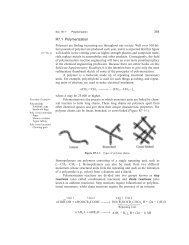
6 is the skew angle of Xs axis. In the meantime, ip turns undefined,
which is also true when the definition of ip is referred in
Figure 4.
To solve for the initial extrinsic parameters of the system,
equate the corresponding terms of matrix fT in Eqs. (7) and
(8), twelve equations are found. Solving the 12 simultaneous
equations, we have
aa = tan" 1 [(tl3t32 - t^h^lih^ - t23tn)]
(30 = cos" 1 Mi + '33
, y„ = tair'tez/fss)
(14)
Subsequent angular motions of the pan-tilt device can be measured
by the angular encoder as Aa, A/?, Ay. Then the current
roll-pitch-yaw angles become a = a0 + Aa, p = /3a + A/3, y
= yD + Ay. Knowing these angles, a new transformation matrix
can be readily calculated from (7), thus saving subsequent
calibrations.
4 Sensitivity Analysis of Dimensional Deformation
The nonhomogeneous coordinate transformation of the laser
scanning process is not a shape and dimension preserving transformation.
In this section, sensitivity analysis of deformation
due to the two skew angles are performed by computer simulation.
4.1 Euclidean Length Deformation. Given two arbitrary
points P,(x[, y\, z[) and P2(^2, yk, Z2) in a 3D Cartesian
space, e.g., the imaginary Cartesian sensor frame {S'}, it is of
interest to know how the distance between the two changes
after the nonhomogeneous coordinate transformation. The coordinates
of the same two points in the true skewed sensor frame
598 / Vol. 118, NOVEMBER 1996
{S} can be calculated from Eq. (3) as Pi (xt, yx, Z\) and P2 (x2,
y2,z2). If the distance between the two points in Cartesian space
is d\2, after the transformation of Eq. (4), the length deformation
is
where
Adn(6, i},) = U\l + Dl2(d, i//) - d[2
Dn(0,