matemática - Blog de ESPOL - Escuela Superior Politécnica del Litoral

+ O
3
( ξ )
STARTING HOMOCLINIC TANGENCIES NEAR 1:1 RESONANCES
⎛ξ1⎞ ⎛ξ1+ ξ2
⎞
⎜ ⎟Nν( ξ)
: = ⎜ 2
ξ ⎜ ⎟
2 ξ2+ ν1+ ν2ξ2+ A( ν) ξ1 + B(
ν) ξξ ⎟
⎝ ⎠ ⎝ 1 2⎠
where A( ) , B(
)
ν : ( ν1, ν2)
2
A( 0, ) B( 0) 0, ξ1,2
,
⋅ ⋅ depend smoothly on
= ∈ , and
≠ ∈ . This normal form
can be approximated by the flow of a vector field
for all sufficiently small ν , that is
1
2 2 3
( ξ) ϕ ( ξ) ( ν ) ( ξ ν ) ( ξ )
N = + O + O + O ,
ν ν
t
where ϕ ν is the flow of a smooth planar system,
whose dynamics are described by the Bogdanov-
Takens bifurcation theory. Therefore, a tangential
homoclinic orbit of the normal form can be
approximated by a homoclinic orbit of the vector
field, for which several starting procedures are
available, see e.g. [3]. Once we have constructed
an approximating homoclinic orbit for the normal
form of the 1 : 1 resonance, we can transform this
orbit to an approximating orbit for a general
system (1), via numerical center manifold
reduction. For this purpose, the homological
equation (cf. [2]) plays a central role. This
equation has the form
f ( H( ξ, ν) , K( ν) ) = H( Nν( ξ) , ν)
,
(2)
2 2 N
where H : × →
and
2 2
K : → are locally defined, smooth
functions that represent a parametrization of a
center manifold of (1) and a parameter
transformation, respectively. By (2), we can
obtain linear approximations of the functions H,K,
and hence a homoclinic orbit of the normal form
can be transformed into an approximating
homoclinic orbit of the general system (1). The
resulting starting procedure can be found in [4].
22
3. NUMERICAL EXAMPLES
Consider the following three-dimensional
version of the Hénon map
2
⎛x⎞ ⎛α2 + α1z−
x ⎞
⎜y⎟ ⎜ ⎟
⎜
x
⎟
,
⎜ ⎟
⎝z⎠ ⎜ y ⎟
⎝ ⎠
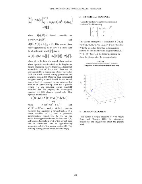
This system undergoes a 1: 1 resonance at (x,y, z)
= (−0.75,−0.75,−0.75), (α1,α2) = (−0.5,−0.5625).
With the procedure described in the previous
section, we find a homoclinic tangency at (α1,α2)
≈(−1.144,−0.233). In the following picture we
show the phase plot of the computed orbit.
FIGURE 1
Starting homoclinic tangencies near 1:1 resonances
Tangential homoclinic orbit of the h´enon map
4. ACKNOWLEDGMENT
The author is deeply indebted to Wolf-Jürgen
Beyn and Thorsten Hüls for stimulating
discussions and suggestions about the present
work.