Editorial - Universidad Autónoma del Estado de México

UNIVERSIDAD AUTÓNOMA DEL
ESTADO DE MÉXICO
Dr. en C. Eduardo Gasca Pliego
Rector
M.A.S.S. Felipe González Solano
Secretario de Docencia
Dr. en Fil. Sergio Franco Maass
Secretario de Investigación y
Estudios Avanzados
Dr. en C. Pol. Manuel Hernández
Luna
Secretario de Rectoría
M. A. E. Georgina María
Arredondo Ayala
Secretaria de Difusión Cultural
M. en A. Ed. Yolanda E.
Ballesteros Sentíes
Secretaria de Extensión y Vinculación
Dr. en C. Jaime Nicolás Jaramillo
Paniagua
Secretario de Administración
Dr. en Ing. Roberto Franco Plata
Secretario de Planeación y Desarrollo
Institucional
Profr. Inocente Peñaloza García
Cronista
Dr. en D. Hiram Raúl Piña Libien
Abogado General
L. en Com. Juan Portilla Estrada
Director General de Comunicación
Universitaria
C.P. Ignacio Gutiérrez
PadillaContralor Universitario
Facultad de Economía
M. en E. Joel Martínez Bello
Director
L. en E. Octavio C. Bernal Ramos
Subdirector Académico
L. en A.F. María de Lourdes Casas Hinojosa
Subdirectora Administrativa
M. en E. Leobardo de Jesús Almonte
Coordinador de Investigación y Estudios
Avanzados
L. en R.E.I. Esmeralda Herrera Romero
Coordinadora de Planeación y Desarrollo
Institucional
L. en R.E.I Jeanett Campos Chávez
Encargada de la Coordinación de Difusión
Cultural
M.E.U.R. Esteban F. Sánchez Torres
Coordinador de Extensión y Vinculación
L. en E. Sandra Ocho Díaz
Coordinadora de la Licenciatura en Economía
M. en D.N. Noelly Karla Sarracino Jiménez
Coordinadora de la Licenciatura en Relaciones
Económicas Internacionales
L. en A. F. María Regina Serrano Crivelly
Coordinadora de la Licenciatura en Actuaría
L. en E. Roberto Ibarra Suarez
Jefe del Departamento de Control Escolar
L. en E. Eloy Carbajal Flores
Jefe del Departamento de Servicio Social
L. en E. María Guadalupe Ramírez Pareja
Jefe del Departamento de Evaluación Profesional
y Seguimiento de Egresados

Instrucciones para colaboradores
Los artículos presentados a Paradigma Económico deberán tratar algún tema teórico o empírico relacionado
con la economía regional y sectorial. La revista está abierta a diferentes enfoques y metodologías.
Los artículos recibidos serán objeto de una evaluación preliminar por el comité editorial y el editor, quienes
determinarán la pertinencia para continuar con el proceso de arbitraje. No se aceptarán trabajos que no consideren
explícitamente como componente relevante la economía regional y sectorial.
El artículo que cumpla con los requisitos temáticos, además de los requisitos formales, será enviado de
manera anónima a dos árbitros para su dictamen. En caso de discrepancia entre ambos dictámenes, el artículo
será enviado a un tercer árbitro, cuya decisión definirá su publicación. Los resultados del proceso de dictamen
académico serán inapelables en todos los casos.
1. El envío de un artículo supone la obligación del autor
de no someterlo simultáneamente a la consideración
de otras publicaciones. Se deberá adjuntar una
carta dirigida al editor de Paradigma Económico en
la que se proponga el artículo para su publicación y
se declare que es inédito y que no está siendo presentado
en otro medio.
2. La colaboración debe ajustarse a las siguientes normas.
De no cumplirse con ellas, no se considerará
para su publicación.
a). Incluir la siguiente información: i) Título del trabajo,
de preferencia breve, sin sacrificio de la claridad;
ii) un resumen de su contenido en español e inglés
de 40 a 80 palabras o 10 líneas aproximadamente,
la clasificación JEL y de tres a cinco palabras clave;
iii) nombre e institución a la que pertenece el autor,
con un breve currículum académico y profesional;
iv) domicilio, teléfono, correo electrónico, fax u otros
datos que permitan la comunicación con el autor.
b). Presentarse en archivos de texto en Word para Windows
en letra Times New Roman, tamaño 12, a doble
espacio. Los cuadros y gráficas en Excel para Windows,
indicando el espacio donde se insertarán así
como el nombre de cada uno (un archivo por cada
cuadro o gráfica).
c). Extensión máxima de 35 cuartillas, incluyendo cuadros,
gráficas y otros apoyos.
d). Se debe proporcionar, la primera vez que se citen,
la equivalencia completa de las siglas empleadas
en el texto.
e). Se admitirán trabajos en español, inglés o portugués.
f). Deberán hacerse siempre las referencias bibliográficas
que correspondan al texto. De no ser así e
incurrirse en plagio intelectual o de cualquier índole,
Paradigma Económico no asumirá ninguna responsabilidad
y, por lo tanto, el autor tendrá que hacer
frente a las leyes correspondientes.
g). Los trabajos deberán ser escritos cuidando las normas
de ortografía y redacción, cumpliendo con las
siguientes características generales:
• Las notas a pie de página deberán utilizarse sólo
si es absolutamente necesario y con interlineado
sencillo.
• Para las referencias dentro del texto se usará la notación
Harvard.
• Las referencias bibliográficas se ordenarán alfabéticamente
al final del texto, con todos los elementos
de una ficha de la siguiente forma: i) Apellido y
nombre del autor; ii) título del artículo (entrecomillado)
y título de la revista o libro donde apareció (en
cursivas) o título del libro (en cursivas); iii) editorial;
iv) ciudad; v) año de edición del libro o volumen, número
y fecha de la revista; vi) número de páginas o
páginas de referencia.
• Para los sitios web se incluirá la ruta completa del
trabajo indicando la fecha de consulta, por ejemplo:
Pérez, A. (2004). “Un modelo de pronóstico de la
formación bruta de capital privado de México”, Documento
de investigación. No. 2004-4. Banco de
México, México. (17 de noviembre de
2004).
• En el caso de artículo en revista, capítulo de libros,
etc., que se consulten en la web se usa el mismo criterio
de una referencia normal y además se incluye
la ruta completa del trabajo y la fecha de consulta.
3. En el caso de los trabajos aceptados para publicarse,
la revista se reserva el derecho de editarlos,
imprimirlos, reimprimirlos y difundirlos en versión impresa,
electrónica y en medios magnéticos.
4. Paradigma Económico se reserva el derecho de
hacer los cambios editoriales que considere convenientes.
Revista Paradigma Económico
Facultad de Economía. UAEMex
Cerro de Coatepec s/n. Ciudad Universitaria
Toluca, México. C.P. 50100
Tel. +52 (722) 214 94 11
Tel. y Fax +52 (722) 213 13 74
Correo-E: paradigmaeconomico@uaemex.mx
http://www.uaemex.mx/feconomia/publicacion_
paradigma.php

Editorial
En un artículo publicado en 2006, 1 Roberta Capello deja
ver su visión optimista sobre el futuro de la economía
regional, e insiste en que los especialistas en estos temas
siguen teniendo ante sí algunos desafíos teóricos a los que hay que
hacerles frente. Entre ellos el intento por obtener ventajas de una
futura convergencia en los diferentes enfoques teóricos que, a decir
de la autora, esa convergencia sólo se ha conseguido parcialmente
por las nuevas teorías del crecimiento regional.
En este sentido, destaca que “en el proceso de globalización
de la economía, los factores locales y sus especificidades son
elementos fundamentales de los que depende la competitividad de
los países y, en consecuencia, representan áreas importantes en las
que los profesionales y los policy makers requieren de un instrumental
sofisticado y avanzado para poder intervenir” (pág. 189).
De acuerdo con esta idea, presentamos el número 1 del año 3
de Paradigma Económico convencidos de que serán los estudios
que aborden los impactos sectoriales y regionales en el contexto
de apertura y liberalización comercial y financiera, los que puedan
proponer estrategias para aprovechar las ventajas que ofrece la
economía global en términos de la expansión de la producción y
la generación de empleos, así como del mejoramiento constante
de la competitividad del aparato productivo y de los espacios,
nacionales y estatales.
En este número, Pablo Mejía y Diana Lucatero analizan la dinámica
de largo plazo del pib de México y de sus 32 estados para
el periodo 1940-2006, con el fin de determinar si las series son
estacionarias una vez que son incorporados uno y dos quiebres
estructurales. Las principales conclusiones a las que llegan es que
1. Capello, R. (2006). “La economía regional tras cincuenta años: desarrollos teóricos
recientes y desafíos futuros”, Investigaciones regionales. Núm. 009. Asociación
Española de Ciencia Regional. Alcalá de Henares, España.

la producción es estacionaria en torno a una tendencia determinista
segmentada en catorce de treinta y tres casos analizados; que los
quiebres estimados pueden asociarse a las distintas estrategias de
crecimiento aplicados en México en las décadas pasadas; y que ha
habido una reducción generalizada de largo plazo en las tasas de
crecimiento de los estados.
Roberto Ramírez y Alfredo Erquizio, a partir del método de
regresión de frontera estocástica para datos de panel, miden la
capacidad y el esfuerzo de recaudación de impuestos e ingresos
propios por entidad federativa. Comprueban que los determinantes
socioeconómicos del esfuerzo fiscal no operan en la misma dirección
y con la misma intensidad para impuestos y para ingresos
propios. Zeus S. Hernández, Gonzalo Dolores de la Merced y
César Amador, rescatan las observaciones señaladas por el Instituto
Nacional de Estadística y Geografía, de México, sobre la comparación
inadecuada de indicadores derivados del Sistema de Cuentas
Nacionales y los obtenidos a partir de los censos económicos por
entidad federativa, como el producto interno bruto, la producción
bruta total y el valor agregado censal bruto, debido esencialmente
a cuestiones metodológicas, conceptuales y de cobertura. Evalúan,
mediante pruebas no paramétricas, la asociación estadística entre
indicadores que presentan discrepancias y las consecuencias que
pueden generar en el cálculo de indicadores regionales y, más aun,
en la estimación de modelos econométricos.
Finalmente, Liliana Rendón y Francisco Herrera documentan la
importancia que tienen las organizaciones y las asociaciones como
promotoras del desarrollo endógeno a través del cultivo de nopal
en los municipios de San José del Rincón y Villa Victoria, Estado
de México.
Leobardo de Jesús Almonte
Director Editorial

Año 3 Núm. 1 enero-junio 2011
Contenido
Trends, structural breaks and economic growth
regimes in the states of Mexico, 1940-2006
Pablo Mejía Reyes and Diana Lucatero Villaseñor
Capacidad y esfuerzo fiscal en las entidades
federativas en México: medición y determinantes
Roberto Ramírez Rodríguez y Alfredo Erquizio Espinal
Fundamento metodológico, discrepancias
estadísticas y errores conceptuales en el uso
de datos económicos
Zeus Salvador Hernández Veleros, Gonzalo Dolores de la
Merced y César Amador Ambriz
Hacia el desarrollo endógeno en el Estado de
México, a través del cultivo de nopal
Liliana Rendón Rojas y Francisco Herrera Tapia
5
37
71
78
PARADIGMA ECONÓMICO REVISTA DE ECONOMÍA REGIONAL Y SECTORIAL FA-
CULTAD DE ECONOMÍA DE LA UNIVERSIDAD AUTÓNOMA DEL ESTADO DE MÉXI-
CO, Año 3, No. 1, enero – junio 2011, es una publicación semestral editada por la Universidad
Autónoma del Estado de México, a través de la Facultad de Economía. Cerro de Coatepec s/n,
Ciudad Universitaria, C.P. 50100, Toluca, Estado de México. Tel. (722) 2 14 94 11 y 2 13 13 74,
correo electrónico: paradigmaeconómico@uaemex.mx. Editor responsable: Leobardo de Jesús
Almonte. Reservas de Derechos al Uso Exclusivo No. 04-2010-073014022200-102, ISSN: en
trámite. Licitud de Título y Contenido No. 14988 otorgado por la Comisión Calificadora de
Publicaciones y Revistas Ilustradas de la Secretaría de Gobernación. Impresa por Litho Kolor,
S.A. de C.V. Vialidad las Torres No. 605, Colonia Santa María de las Rosas, C.P. 50140, Toluca,
Estado de México, este número se terminó de imprimir el 28 de octubre de 2011 con un
tiraje de 500 ejemplares.
Las opiniones expresadas por los autores no necesariamente reflejan la postura del editor de
la publicación.
Se autoriza la reproducción y/o utilización de los materiales haciendo mención de la fuente.

Instructions for Contributors
Works submitted to Paradigma Económico must refer to a theoretical or empirical topic related to sector and
regional economics. Different methodologies and approaches are well received.
All works, will be subject to pre evaluation by the Editor and the Editorial Board, who will determine the relevance
to continue with the publication process. Works that do not consider the relevancy of regional and sector
economics will not be accepted.
If the article meets the topic and formal requirements, it will be sent anonymously to two different referees for
its evaluation. In case of discrepancy between the two opinions, the article will be sent to a third referee who will
determine define its publication. In all cases, the results of the referee’s opinions will be final.
1. All works submitted in Paradigma Económico
should not be simultaneously submitted in other
publications, a letter to the editor that provides the
originality of the topic should be attached.
2. Contributions must suit the following rules,
otherwise will not be considered for publication:
a) Works must include the following information:
i) A short and understandable title; ii) An abstract
in Spanish and English between 40 and 80 words
and approximately 10 lines, JEL classification and
3 to 5 keywords; iii) Author´s working place and a
brief academic and professional curriculum vitae;
iv) Contact information that allows Paradigma Económico
easy access to the author (address, telephone
number, fax, postal and e-mail address).
b) All articles must be sent files in Word for Windows,
in Times New Roman 12-point font and double spaced
(2.0). Charts, and graphs must be attached in
Excel for Windows indicating where they must be
placed.
c) Must not exceed 35 pages including charts and
graphs.
d) Acronyms must be defined at least the first time
they were mentioned.
e) Articles written in Spanish and English are accepted.
f) References must match with the text, otherwise in
case of plagiarism Paradigma Económico will not
assume any responsibility.
g) Articles must be written following the spelling and
writing rules and general characteristics such as:
• Use footnotes only if necessary and using single
space.
• For references appearing in the text itself, the Harvard
notation system will be used.
• References must be ordered alphabetically at the
end of the text with the following data: i) Author´s
surname and first name; ii) Year of publication (in
parentheses); iii) Title of the article (in quotation
marks); iv) Name of the journal or book (in italics),
v) Editor, vi) Date number and volume; vii) City and
country where published.
• For web sites, the full internet direction and the
consultation date must be specified. For example:
Pérez, A. (2004). “Un modelo de pronóstico de la
formación bruta de capital privado de México”, Documento
de investigación. No. 2004-4. Banco de
México, México. http://www.banxico.gob.mx/gPublicaciones/DocumentosInvestigacion/docinves/
doc2004-4/doc2004-4.pdf> (17 de noviembre
de2004).
• In case of magazine articles, book chapters, etc.,
consulted on the internet, they must be referred
as normally including the the full internet direction
and the consultation date
3. For articles accepted, Paradigma Económico reserves
the right to edit, print and reprint the articles in
paper, electronic and magnetic version
4. Paradigma Económico reserves the right to make
editorial and editing corrections if necessary.
Revista Paradigma Económico
Facultad de Economía. UAEMex
Cerro de Coatepec s/n. Ciudad Universitaria
Toluca, México. C.P. 50100
Tel. +52 (722) 214 94 11
Tel. y Fax +52 (722) 213 13 74
Mail: paradigmaeconomico@uaemex.mx
http://www.uaemex.mx/feconomia/publicacion_
paradigma.php

Paradigma Económico se publica dos veces al año por la Facultad de
Economía de la Universidad Autónoma del Estado de México. Aborda
temas relacionados con la economía regional y sectorial, y está abierta
a diferentes enfoques y metodologías.
El Comité Editorial con el apoyo de una cartera de árbitros, nacional
e internacional, dictamina anónimamente los trabajos recibidos
para evaluar su publicación. El resultado es inapelable en todos los
casos. El contenido de los artículos que aparecen en cada número es
responsabilidad exclusiva de los autores y no expresa necesariamente
la opinión de la institución.
Los trabajos que se entreguen a Paradigma Económico para su
publicación deberán ser inéditos, de carácter eminentemente académico
y ajustarse de manera estricta a las normas editoriales que se indican
en las Instrucciones para colaboradores que se incluye en la revista.
PARADIGMA ECONÓMICO
Comité editorial
Leobardo de Jesús Almonte
Patricio Aroca, Universidad Católica del
Director Editorial
Norte, Chile.
Alejandro Dávila Flores, Centro de
Investigaciones socioeconómicas,
Universidad de Coahuila.
Christine Cartón Madura, División de
Ciencias Sociales y Administrativas,
Universidad de Quintana Roo.
Cuauhtémoc Calderón Villarreal,
Departamento de Estudios Económicos, El
Colegio de la Frontera Norte.
Laura E. del Moral Barrera, Facultad de
Economía, UAEMéx.
Luis Quintana Romero, FES Acatlán, UNAM.
Miguel Ángel Díaz Carreño, Facultad de
Economía, UAEMéx.
Normand Assuad Sanen, Facultad de
Economía, UNAM.
Pablo Mejía Reyes, Facultad de Economía,
UAEMéx.
Reyna Vergara González, Facultad de
Economía, UAEMéx.
Zeus Salvador Hernández Veleros, Instituto
de Ciencias Económico-Administrativas,
Universidad Autónoma del Estado de Hidalgo.
Asistente editorial
Brenda Murillo Villanueva
Formación y diseño
Alejandra Santana Castro
Corrección de estilo
Edith Muciño Martínez
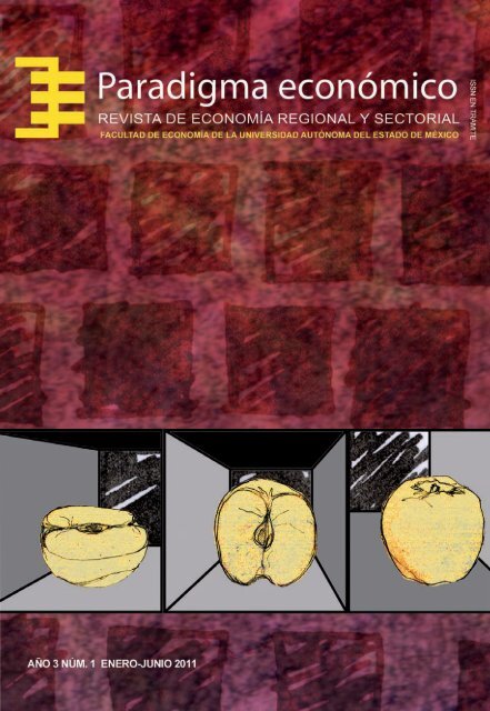
Portada: Análisis de un problema.
En este número se hace referencia a la
forma de analizar un problema y dividirlo
en las partes que lo conforman,
incluso poder apreciarlo en varias perspectivas
y ángulos, es decir, contemplar
todas sus dimensiones.
La expresión gráfica del logotipo
representa en las tres plecas horizontales
a los tres sectores productivos. El gráfico
que los cruza es la expresión del análisis
económico, cuyo fin es observar los datos
que se generen en la actividad económica
de los tres sectores para proyectar un
panorama de análisis y discusión.

Paradigma económico Año 3 Núm. 1 enero-junio 2011
Págs: 111-140
Hacia el desarrollo endógeno
de las comunidades mazahuas del
Estado de México. Contribuciones
a partir de la producción de nopal
Liliana Rendón Rojas* y Francisco Herrera Tapia**
Resumen
Se pretende documentar la importancia que tienen las organizaciones y las
asociaciones como promotoras del desarrollo endógeno a través del cultivo
de nopal en los municipios de San José del Rincón y Villa Victoria, Estado
de México. Se muestran indicios que inciden favorablemente en el desarrollo
local y en la generación de nuevas estrategias de crecimiento económico a
partir de este producto y que merecen ser estudiadas. Inicialmente, el proyecto
del nopal surge como una opción para incidir positivamente en la seguridad
alimentaria de las familias, no obstante, el excedente de producción vino a
influir en el mercado regional y en otros aspectos del desarrollo comunitario,
lo cual confirma un efecto multiplicador endógeno de actividades económicas
y no económicas derivadas de la producción intensiva y sustentable del nopal.
Proyecto que no hubiera existido sin la intervención de los agentes externos,
y sin la participación proactiva de la población.
Palabras clave: desarrollo endógeno, local, capital social, Estado de
México y cultivo de nopal.
Clasificación JEL: O13, O18, P31, P32, R51.
Abstract
Towards endogenous development of the mazahuas of the State of
Mexico communities. Contributions from the production of nopal
The objective of this paper is to document the importance of the organizations
and associations as promoters of the endogenous development
through the cultivation of nopal in the municipalities of San José del
* Profesora de la Facultad de Economía de la Universidad Autónoma del Estado
de México. Correo electrónico: lila-rendon@hotmail.com.
** Profesor-Investigador del Instituto de Ciencias Agropecuarias y Rurales de
la Universidad Autónoma del Estado de México. Correo electrónico: fherrerat@
uaemex.mx.
recepción: 4/03/2011 aceptación: 17/08/2011
[111]

112 Paradigma económico Año 3 Núm. 1
Rincón and Villa Victoria, Mexico State. It is being shown evidence
that affect favourably in local development and generating new strategies
of economic growth from this product and they deserve to be
studied. Initially, the project of the nopal emerges as an option for positively
influencing the food security of families, however, the surplus of
production came to influence the regional market and in other aspects
of community development, which confirms an endogenous multiplier
effect of economic and non economic activities resulting from the intensive
and sustainable production of the Nopal (Cactus). Project that
would not have existed without the intervention of external actors, and
the proactive participation of the population.
Key words: Endogenous development, local, social capital, State of Mexico
and cultivation of Nopal.
Introducción
El desarrollo económico de una localidad genera un amplio
debate: se promueve la discusión sobre qué es lo que genera dicho
proceso y por qué. En este sentido, el desarrollo endógeno es una
teoría explicativa para analizar por qué las regiones ven aumentada
su producción, productividad e innovación, generando con
ello desarrollo hacia adentro de las mismas.
Este tipo de desarrollo es atribuido a factores internos, generados
a partir de transformaciones en los modos de producción,
inversiones locales y aumento en la modernización tecnológica.
La teoría del desarrollo endógeno, en general, atribuye un papel
determinante a la sociedad y a las organizaciones que actúan en
el ámbito local, dando un papel de promotor de sus capacidades y
generando el cambio de abajo hacia arriba.
De acuerdo con autores como Boisier (1998), Berumen
(2006) y Vázquez (1999), entre otros, podemos partir del
siguiente supuesto: el crecimiento de largo plazo, generador
del desarrollo económico de las localidades perteneciente a
un país, está basado en incentivos económicos proporcionados
por el ambiente en el cual los agentes económicos trabajan. Se
atribuye más importancia a las instituciones y organizaciones
locales que a las políticas regionales implementadas desde el

Hacia el desarrollo endógeno de las comunidades... Rendón, L. y Herrera F.
113
centro, sus seguidores promueven una autonomía más generosa
de las regiones.
Bajo este contexto, el objetivo de este trabajo es documentar
la importancia que tienen las organizaciones sociales y las asociaciones
como promotoras del desarrollo endógeno a través del
cultivo de nopal orgánico mediante 85 invernaderos, pertenecientes
a los municipios de San José del Rincón y Villa Victoria,
Estado de México. Éstos tienen capacidad de producción de poco
más de 500 kilos mensuales, que se convierten en ingreso para las
familias mazahuas. Bajo la perspectiva del crecimiento económico,
estos datos empíricos inciden favorablemente en el desarrollo
local a través de externalidades positivas y en la generación
de nuevas estrategias de crecimiento económico a partir de este
producto, que merecen ser estudiadas.
Con estos planteamientos, este trabajo se estructura de la
siguiente manera: en el primer apartado se plantea la conceptualización
de la teoría del crecimiento económico regional y
la teoría de desarrollo endógeno. En el segundo apartado se
muestra cómo el desarrollo endógeno atribuye a los actores
e instituciones, la capacidad de lograr políticas regionales de
beneficio económico, utilizando las fortalezas y el contexto
físico-ambiental; se rescata el papel local del municipio como
clave de desarrollo en esta nueva faceta de desarrollo desde
abajo, donde el entorno local es revalorado, considerando a las
organizaciones y agentes productivos. En el tercer apartado se
muestra el caso de los mazahuas, a partir del rescate de la experiencia
de la organización civil: Fundación Mexicana para el
Desarrollo Rural A.C, (sedemex) y su incidencia en la producción
de nopal bajo invernadero en los municipios: San José del
Rincón y Villa Victoria, del Estado de México, donde se ha
logrado incidir positivamente en la seguridad alimentaria y en
algunas vertientes del desarrollo endógeno de localidades atendidas
por esta organización social.

114 Paradigma económico Año 3 Núm. 1
1. La teoría del desarrollo endógeno
En los años setenta el desarrollo de las naciones se entendía como
la capacidad de una economía para generar y sostener el aumento
anual de su Producto Interno Bruto (pib) a una tasa de 5 a 7%
o más, actualmente implica más que sólo crecimiento económico.
El desarrollo debe concebirse entonces, como un proceso
multidimensional que implica cambios de las estructuras, actitudes
e instituciones, al igual que la aceleración del crecimiento
económico, la reducción de la desigualdad y la erradicación de la
pobreza absoluta (Todaro, 1982).
Es así como el desarrollo está fuertemente vinculado con el
crecimiento económico. No puede haber desarrollo sin crecimiento,
pero debemos entender que son dos cosas distintas. El
desarrollo económico es producto de las políticas públicas instrumentadas
por el gobierno, las instituciones y las organizaciones a
través de los ciudadanos y actores sociales. Cuando hablamos de
una sociedad desarrollada estamos pensando en una sociedad en
la que las diferencias económicas disminuyen y existe un mejor
entorno social para todos: incluye derechos humanos, estabilidad
de precios, alto índice de alfabetización y en general un bienestar
amplio para la sociedad (Debraj, 1998).
A su vez, todos los modelos de crecimiento tienen la siguiente
implicación: los cambios en las políticas gubernamentales, como
subsidios a la investigación o impuestos sobre las inversiones,
tienen efectos de nivel pero no de crecimiento de largo plazo, es
decir, estas políticas elevan temporalmente la tasa de crecimiento:
la economía crece a un nivel más alto de la ruta de crecimiento
equilibrado, pero a largo plazo la tasa de crecimiento regresa a
su nivel inicial. Originalmente se usó el término “crecimiento
endógeno” para referirse a modelos donde los cambios de esas
políticas pudieran influir sobre la tasa de crecimiento en forma
permanente (Jones, 2000: 149).
Las teorías económicas han sufrido cambios, surgen nuevas
circunstancias para los mercados y para los factores de la producción;
las nuevas tecnologías y el fenómeno de la globalización

Hacia el desarrollo endógeno de las comunidades... Rendón, L. y Herrera F.
115
desencadenan en cascada cambios en las teorías económicas,
pasando del crecimiento económico al paradigma del desarrollo
económico. Este nuevo paradigma está relacionado con el denominado
“desarrollo endógeno”.
Uno de los autores más representativos del desarrollo endógeno
es Antonio Vázquez Barquero, quien destaca en sus explicaciones
teóricas, que el sistema productivo de los países crece y
se transforma utilizando el potencial de desarrollo existente en el
territorio (en las regiones y en las ciudades) mediante las inversiones
que realizan las empresas y los agentes públicos, bajo el
control creciente de la comunidad local (Vázquez, 1999).
Por su parte Boisier (1998), plantea que el desarrollo de una
nación implica elementos como: educación, nivel de vida, capacitación
para el trabajo, competitividad y en general una transformación
cultural de los ciudadanos involucrados. Además está vinculada
de manera directa con el entorno territorial, donde la calidad de
dicho territorio determina el desarrollo de las estructuras sociales.
Este nuevo esquema económico que tiene como objetivo
explicar la naturaleza económica y adoptar un modelo a seguir,
surge por el agotamiento de los postulados desde afuera que planteaban
los neoclásicos en la década de los sesenta y setenta, ahora
se propone un desarrollo desde adentro. Esto se logra con la vocación
de las comunidades hacia negocios o explotación de recursos
naturales, culturales, turísticos e industriales. La clave del desarrollo
está en el proceso complejo y permanente de coordinación
de decisiones que pueden ser tomadas por una multiplicidad de
agentes, cada uno de los cuales puede incidir en los factores de la
producción (Boiser, 1998: 7).
Es decir, ahora el desarrollo lo podemos entender como
endógeno, atribuido a factores internos, propios del territorio y
generados a partir de las inversiones locales y el aumento de la
productividad generada por las innovaciones tecnológicas. Este
es un nuevo esquema que sustenta la importancia del gobierno
local como motor del desarrollo y promotor de inversiones.
Asimismo, conviene recalcar las diferencias entre las teorías
de crecimiento y desarrollo endógeno, pues parten de supuestos

116 Paradigma económico Año 3 Núm. 1
distintos y en ocasiones antagónicos. La teoría del desarrollo
endógeno es territorial, pues tiene capacidad de inversión y
localización de las empresas, también plantea que las formas de
organización de las empresas y el territorio juegan un papel determinante
en los procesos de desarrollo, asumiendo que esto generará
innovación y productividad. Además en esta nueva teoría se
plantea a la sociedad como un motor de desarrollo, a través de sus
lazos con las empresas, con el gobierno y con las organizaciones.
Por su parte, la teoría del crecimiento económico regional se
basa en el supuesto de que el crecimiento de largo plazo se deriva
de los incentivos económicos proporcionados por el ambiente
dentro del cual los agentes económicos trabajan. Además otorga
mayor importancia a las instituciones locales que a las políticas
regionales implementadas desde el centro. Sus seguidores
promueven una autonomía administrativa más generosa de las
regiones, al igual que programas de desarrollo regional y estatal
para éstas (Mendoza y Díaz-Bautista, 2006).
El interés de las teorías endógenas del crecimiento económico
se centra en la naturaleza y el papel del conocimiento en el proceso
del crecimiento (Grossman y Helpman, 1990). A diferencia de
los modelos anteriores del crecimiento como el de Solow (1994)
donde el cambio tecnológico apareció como parámetro exógeno;
esta nueva teoría del crecimiento regional ha buscado endogeneizar
el cambio técnico. Los agentes invierten recursos en la investigación
y en el desarrollo, donde de una máquina no sale solamente la
producción, sino nuevos conocimientos tecnológicos.
Arrow en 1962, menciona que el conocimiento tiene ciertas
características peculiares como el de derramarse fácilmente en
las manos de otras personas con un costo marginal cercano a
cero. Este autor también sostiene que las inversiones en capital
físico tendrán en efecto un derrame sobre el nivel de tecnología
del sistema, por la acumulación del conocimiento en
los empleados. Asimismo, Lucas (1988) retoma el papel del
capital humano, en el crecimiento económico y establece que el
aumento del capital humano a través de los procesos de educación
y formación transformará el entorno en el que las empresas

Hacia el desarrollo endógeno de las comunidades... Rendón, L. y Herrera F.
117
realizan sus actividades productivas y de generación de capital
(Sala-i-Martin 2000).
Podemos decir entonces, para el caso de estudio que nos
ocupa, que este proceso de spillovers en la economía es la fuente
que genera el desarrollo económico regional, al igual que Arrow
plantea: la inversión en capital humano redundará en el mejoramiento
del proceso productivo, como consecuencia de afinar las
habilidades y debido a las externalidades asociadas a la existencia
de un entorno económico donde la mano de obra es calificada,
entrenada y por ende más productiva.
De tal forma, la tecnología también es determinante para el
desarrollo endógeno: genera innovaciones tecnológicas, industriales
y empresariales para convertirse en motor del crecimiento.
Schumpeter (1976) postula a la innovación tecnológica como la
fuente de la extensión económica.
El postulado de la teoría de desarrollo endógeno establece
modelos donde toda inversión produce un efecto difusor,
externo a la fuente de producción que la realiza, mejorando la
productividad de la empresa y promoviendo el desarrollo de las
comunidades. Esta teoría atribuye un papel determinante a la
sociedad y específicamente a organizaciones que actúan en el
ámbito local, dando un papel orientado a promover sus capacidades
y generar el cambio de abajo hacia arriba. El capital social
y humano son herramientas del desarrollo aplicables a cualquier
localidad. Las políticas de desarrollo local serán por tanto, más
importantes que establecer una agenda general o aplicable a
todo el territorio.
Las teorías del desarrollo endógeno son particularmente
especiales, dado que reconocen la existencia de rendimientos
crecientes de los factores acumulables y las inversiones en capital
físico, capital humano e investigación y desarrollo de economías
externas, permitiendo identificar una senda de desarrollo económico
autosostenido, de carácter endógeno en la productividad
local o regional.
Ante esta circunstancia, el desarrollo endógeno es un esquema
planteado como opción ante el desequilibrio económico docu-

118 Paradigma económico Año 3 Núm. 1
mentado en varios países incluyendo México. Los procesos de
acumulación de capital, de innovación y de formación de capital
social tienen un carácter localizado (Moncayo, 2003).
Coincidente con otros autores, Sergio Boiser (1998) y Debraj
(1998) señalan que el entorno territorial es factor clave del desarrollo.
Bajo diferentes fórmulas administrativas y jurídicas del
entorno territorial: la comuna, la provincia, la región y la calidad
de éstos determina el desarrollo de las estructuras sociales pertinentes
en cada escala. Esto significa que ahora la planeación
económica está partiendo de un paradigma de abajo hacia arriba
y no al revés, como se estuvo trabajando durante mucho tiempo
para establecer políticas públicas.
El territorio, un elemento fundamental para la creación del
Estado bajo la teoría de desarrollo endógeno, ofrece una visión
distinta del uso que se le da al espacio público, considerándolo
como un punto de encuentro entre los intereses y las capacidades
que se generan a partir de una visión o estrategia compartida.
De esta manera, el entorno local está siendo revalorado, pero
también el territorio pues la localización industrial y el desarrollo
de productos en determinado espacio físico es lo que determina
la productividad y el desarrollo de la mano de obra. Lo local es
el punto de encuentro de esa fuerte y particular relación entre
territorio y desarrollo: el ámbito donde los actores dejan de ser
espectadores y pasan a ser protagonistas.
2. Capital social y organizaciones promotoras
del desarrollo
Actualmente se ha generado un concepto nuevo, para definir la
estrategia que toma las oportunidades de la globalización para
explotarlas en el entorno local. Pensar global y actuar local es la
propuesta que se denomina: glocal (Berumen, 2006:37). Se plantea
bajo este esquema que las comunidades y localidades deben
adaptarse a las exigencias de la globalización, asimilando nuevos
conocimientos y aprovechando las nuevas tecnologías y recursos
disponibles para estar a la altura del orden mundial.

Hacia el desarrollo endógeno de las comunidades... Rendón, L. y Herrera F.
119
De tal forma que los individuos en el entorno local, junto
con las organizaciones e instituciones multinacionales, estatales,
locales e incluso virtuales son agentes de cambio. Y es en el entorno
local donde se genera un esquema de competencias para lograr un
esquema de desarrollo. Madoery (2001) sostiene que las localidades
adquieren una dinámica de innovación y adaptación a través
de las vocaciones emprendedoras locales y regionales.
Ante la hegemonía que produce la globalización, las redes e
interacciones sociales han adquirido importancia en el proceso
de desarrollo, donde las ciudades y regiones adquieren responsabilidades
tradicionalmente concentradas en el Estado-Nación
(Madoery, 2001). Para Vázquez (2005) los países, las regiones y
las ciudades difieren entre sí por la cantidad y tipo de recursos,
activos económicos, humanos y culturales de que disponen, pero
los ritmos de crecimiento y los niveles de bienestar dependen
sobre todo del desarrollo de las fuerzas que impulsan el crecimiento
y de los efectos de su interacción.
La idea de volver a lo local está presente en estos planteamientos
pues sostienen que la economía depende de factores
focalizados en un espacio físico concreto; ya que aunque se
tengan las mismas condiciones y factores, una región podrá
crecer económicamente más que otra. Los casos de éxito como
Silicon Valley, en California, Jura en Suiza, Turín en Italia y
otras regiones no pueden ser copiadas para otra región simplemente
porque no cuentan con las mismas condiciones, ni los
mismos actores; no puede importarse el éxito económico, habrá
que instrumentar políticas aplicadas a cada entorno.
Madoery (2001) sostiene que el desarrollo endógeno es un
proceso de aprendizaje colectivo, cambio cultural y en general
de prácticas de apropiación simbólica; generada por los propios
actores a partir de sus capacidades.
Cada territorio tiene un conjunto de recursos materiales,
humanos, institucionales y culturales que constituyen su potencial
de desarrollo; y que se expresan a través de la estructura productiva,
el mercado de trabajo, la capacidad empresarial y el conocimiento
tecnológico. Además incluye la infraestructura de soporte

120 Paradigma económico Año 3 Núm. 1
y acogida, el sistema institucional y político, y su patrimonio
histórico y cultural. Sobre estas, bases cada economía articula sus
procesos de crecimiento y cambio estructural, como consecuencia
de la interacción de las empresas y los demás actores económicos
en los mercados, se obtienen resultados muy diferentes que dan
lugar a una gran variedad de situaciones, proyectos y procesos
económicos, sociales y políticos (Vázquez, 2005: 7).
Así, la globalización conducirá a una nueva organización
del sistema de ciudades y regiones, donde las redes tendrán un
papel importante y decisivo en la generación de desarrollo para
las comunidades. Asimismo, el desarrollo territorial se convierte
en algo crecientemente endógeno, que depende de los actores
locales, dado que este modelo de desarrollo económico privilegia
el papel que tienen los ciudadanos y los actores implicados en el
impuso económico que se logra.
Esto significa que la teoría de desarrollo endógeno advierte
sobre la responsabilidad que tienen los empresarios, las organizaciones,
las instituciones, el gobierno y los ciudadanos en el desarrollo
económico y en las oportunidades de crecimiento que se
presentan en los distintos rubros. Esta teoría da un papel activo
a las personas que se integran al proceso, las decisiones pueden
venir desde abajo, de los ciudadanos que conocen los problemas
ignorados por las instituciones que desde arriba, de instituciones.
Una vez que se ha identificado por varios autores el poder que
tiene la sociedad organizada, podemos destacar que autores como
Vázquez Barquero (2005) y Mota (2002), sostienen que existen
nuevos paradigmas para la teoría de desarrollo endógeno como el
denominado “fuerzas de desarrollo”, donde están los ciudadanos
y la sociedad civil organizada.
Dichas fuerzas de desarrollo se dan a partir de la sociedad
civil, que ante la ausencia del Estado o el descuido del mismo,
han impulsado políticas de atención a sus problemas y generado
respuestas adecuadas a cada territorio. El planteamiento es que las
políticas de desarrollo siempre serán más eficaces en la medida en
que los actores involucrados e interesados sean quienes impulsen

Hacia el desarrollo endógeno de las comunidades... Rendón, L. y Herrera F.
121
dichos proyectos, porque el centralismo y las políticas de desarrollo
emanadas de organismos internacionales o producto de
programas nacionales no son los más precisos a la hora de aplicarlos
a las localidades.
La participación de la sociedad en la solución de problemas
está vinculada con las distintas categorías de la organización ciudadana,
también llamadas: acción colectiva, participación organizada
o capital social. Este último término proviene de la investigación
realizada por Robert Putnam que lo conceptualizó como el grado
de confianza existente entre los actores sociales de una sociedad,
las normas de comportamiento cívico y el nivel de asociación que
tienen; porque estos elementos evidencian la riqueza y la fortaleza
de un tejido social específico que está en un territorio.
De acuerdo con Vázquez Barquero (1999), la teoría de desarrollo
endógeno es más que un modelo de análisis; es una interpretación
orientada a la acción, en la que los actores locales a
través de sus decisiones de inversión y de sus iniciativas pueden
impulsar la economía local. El desarrollo endógeno es por tanto,
un espacio para la transformación social donde los principales
actores son:
a) Empresas y organizaciones.
b) La sociedad civil organizada (capital social).
La teoría de desarrollo endógeno parte de una realidad: los
actores sociales, los ciudadanos interesados y las personas que
buscan su bienestar siempre podrán actuar en miras a su beneficio
con el conocimiento que tienen del problema. Además esto significa
que los costos de transacción disminuyen, porque los actores
tienen más información que cualquier organismo o institución. Se
genera con ello capital social, producto de la organización de los
individuos en un fin común.
Dicho capital social adquirió gran importancia a partir de
que organismos internacionales relacionados con el crecimiento
económico como el Banco Mundial, la Comisión
Económica para América Latina y el Caribe, el Banco Interamericano
de Desarrollo y otros, le dieron un gran impulso para

122 Paradigma económico Año 3 Núm. 1
generar programas sociales y de apoyo; produciendo efectos
sobre la reducción de la pobreza y la desigualdad económica
(Mota, 2002).
Desde finales de los años ochenta se dio un impulso muy
importante a los gobiernos municipales, tomando un esquema
abierto a incluir a la población en las decisiones de gobierno y
en general en la solución de los problemas. Además el capital
social expresa el valor de las prácticas informales de conducta
que tienen los ciudadanos, expresando el sentido que tiene la reciprocidad
y la confianza (Echebarría, 2007).
Es importante que la población se reúna en organizaciones
porque genera una sinergia social muy trascendente para todos,
adquiriendo además del capital social, simbólico porque sus
creencias y sus hábitos se toman en cuenta; logrando una democracia
participativa propiciando que los actores se involucren en
los proyectos.
La organización de los ciudadanos genera el desarrollo endógeno
que la teoría postula mediante el esquema de cooperación
social, pues se disminuyen los costos de transacción y se establecen
estrategias cooperativas para llegar a beneficios compartidos
o al equilibrio de las ganancias en el caso de las microempresas
y la producción de productos (Atria et al., 2003).
La teoría del capital social sugiere que a medida que aumenta
el capital social dentro de las redes de participantes en las transacciones
y organizaciones vinculadas con empresas o instituciones
productivas, la disparidad de beneficios se reduce y eleva el nivel
medio de beneficios. De tal forma que volver el entorno local es
reorganizar los elementos del desarrollo a partir de las organizaciones
y la relación existente entre el gobierno, las instituciones
y las empresas. Todos estos elementos forman redes sociales y de
trabajo entre ellos, porque la actividad productiva está basada en
un sistema de relaciones formales e informales entre las empresas
y los actores económicos sociales e institucionales.
Madoery (2001) señala que el espacio de lo local es uno de
los aspectos que las teorías económicas no habían considerado
fuertemente como sí está en los postulados del desarrollo endó-

Hacia el desarrollo endógeno de las comunidades... Rendón, L. y Herrera F.
123
geno. Se han presentado experiencias documentadas donde un
territorio logra un gran desarrollo económico y diferenciado de
otras regiones. Podemos destacar que las microregiones constituyen
espacios donde se manifiestan y difunden los cambios y
transformaciones socioeconómicas.
Los rubros enumerados anteriormente requieren por tanto que
se instrumenten los cambios a partir de estos dos actores. Asimismo,
Vázquez (1999) señala que las ciudades, de diferentes tamaños y
con posicionamientos diversos en el sistema de ciudades, son el
espacio del desarrollo económico, dado que en ellas se potencializan
externalidades y se favorecen los procesos de innovación.
Ahora bien, las ciudades deben generar una dinámica de
crecimiento sostenido a partir de la explotación de sus propias
fortalezas, de tal suerte que las políticas públicas instrumentadas
por el gobierno para desarrollar una región o localidad
serán determinantes en la forma que vayan incorporándose a una
transformación de su producción, así como en el desarrollo del
potencial territorial disminuyendo los costos de transacción de
sus productos, lo cual conlleva a revisar los planteamientos de las
políticas de desarrollo local y regional.
3. Análisis de caso, los mazahuas y el cultivo
de nopal
3.1. Antecedentes
San José del Rincón y Villa Victoria son dos municipios de alta
marginación en el Estado de México, ambos se encuentran entre
los cinco municipios más marginados de la entidad, tienen población
de la etnia mazahua y se consideran comunidades rurales
por su estructura poblacional, condiciones ambientales y vocación
productiva (Ver mapa 1).
A principios de 2005, derivado de los estudios y diagnósticos
realizados en el municipio de San José del Rincón, y con base en
el trabajo participativo con poblaciones mazahuas por parte de la

124 Paradigma económico Año 3 Núm. 1
organización civil sedemex 1 se logró que en una de las comunidades
de dicho municipio (San Miguel Agua Bendita), en alianza
con la Fundación Rigoberta Menchú, se instalaran 15 invernaderos
productores de nopal, que posteriormente en 2010 se convertirían
en una red de 85 invernaderos distribuidos entre los municipios
de San José del Rincón y Villa Victoria, Estado de México.
Mapa 1
Ubicación municipal de referencia
Fuente: Elaboración propia.
Producto de la intervención comunitaria se llevaron a cabo
talleres agronómicos participativos en varias comunidades interesadas
en la producción agrícola y se encontró que el cultivo inten-
1. Se constituyó el 15 de noviembre de 1972. Es una asociación civil que no persigue
fines de lucro, sino promover y auxiliar directa e indirectamente el desarrollo
del país y en especial el de los grupos rurales y urbanos que más lo necesiten. Recibe
financiamiento público y privado para sus proyectos.

Hacia el desarrollo endógeno de las comunidades... Rendón, L. y Herrera F.
125
sivo de nopal bajo invernadero ofrecía la posibilidad de invertir a
pequeña escala con beneficios en términos de seguridad alimentaria,
ahorro de agua y con un excedente comercial de poco más
de dos salarios mínimos diarios para la familia que se favoreciera
con un invernadero. Además se buscaba transformar la cultura de
la zona, organizarlos y promover su participación activa como
Maedory (2001), establece en los ejemplos de otros países.
Si bien los apoyos iniciales fueron gestionados exclusivamente
para el fortalecimiento organizacional, la capacitación y la
instalación de invernaderos, el trabajo de intervención fue acompañado
por una serie de actividades tendientes a elevar la capacidad
de autogestión de la población en relación con las actividades
económicas de las localidades, que previamente se fueron
seleccionadas con base en sus altos índices de pobreza.
Una de las acciones tendientes al mejoramiento de la economía
local partió del supuesto de que la organización es un factor detonante
de todo proceso productivo local, en ese sentido se impulsó
la creación de grupos sociales organizados para la producción,
de los que muchos se convirtieron en Sociedades de Producción
Rural (spr), y otro tanto optó por trabajar en grupos familiares para
la gestión y desempeño en relación con los invernaderos. La organización
como factor de cambio permitió este incipiente esquema
de desarrollo endógeno. Con el tiempo se logró incorporar a
varias organizaciones, tal como Echebarría (2007), concede como
un elemento detonante de transformaciones mayores, al abrir la
participación activa de la población.
En el cuadro 1 se muestra el listado de organizaciones que
lograron constituirse en un periodo de cinco años, desde 2005
que inició el programa hasta el 2010. Algunos de los grupos y spr
lograron por cuenta propia hacer gestiones para la adquisición de
otros activos productivos, y crear fondos de ahorro propios para
la contratación de microcréditos, como fue el caso de San Miguel
Agua Bendita en San José del Rincón. Al mismo tiempo las líderes
de esa comunidad por vez primera se integraron al Consejo Municipal
para el Desarrollo Rural Sustentable de San José del Rincón,
en representación de sus asociados, y en ese sentido podían pugnar

126 Paradigma económico Año 3 Núm. 1
por mayores recursos al campo, así como otros recursos de los ya
disponibles, direccionarlos de manera más equitativa a proyectos
productivos del municipio.
Cuadro 1
Organizaciones constituidas
Nombre de la spr
Mujeres Campesinas de Providencia,
SPR de RL
Las Mujeres por el Sueño del Progreso, SPR
de RL
Unión de Mujeres de los Lobos Segunda Sección,
SPR de RL
Las Mujeres en Busca de un Porvenir, SPR
de RL
Grupo San Francisco de La Loma, SPR de RL
Productores de Ovinos de Santa Cruz del
Tejocote, SPR de RL
Grupo Yondece del Cedro Sur, SPR de RL
Localidad de origen
Providencia
San Jerónimo de los Dolores
Los Lobos Segunda Sección
San Miguel Agua Bendita
San Francisco de la Loma
Santa Cruz del Tejocote
Yondece del Cedro Sur
Fuente: Elaboración propia con base en datos de campo.
La toma de decisiones en manos de las organizaciones es
propia de un fenómeno reciente, documentado en otros países,
pero que en México es todavía nuevo. Se apega a los planteamientos
de la teoría del desarrollo endógeno porque su organización
es promovida por la sociedad y no por el gobierno.
Una vez que los invernaderos adquirieron interés y
probaron su viabilidad, la ampliación llegó a 85 invernaderos
de producción de nopal en 2010, lo cual ya justificaba un eslabonamiento
más a esa cadena productiva, ello hizo necesaria la
introducción de un sinnúmero de capacitaciones relacionadas
con la transformación y valor agregado del nopal. Destacaron
los cursos de gastronomía, que fueron bien recibidos por la
comunidad mazahua; mucho de lo aprendido ahora se refleja
en nuevos platillos de las festividades familiares y comunitarias.
Se innovó también en la transformación de la cultura
en la zona, promoviendo nuevos activos sociales, integrando

Hacia el desarrollo endógeno de las comunidades... Rendón, L. y Herrera F.
127
capacidades y vocaciones productivas que privilegian el crecimiento
económico desde las comunidades.
La producción se elevó (a más de 50 000 kg de nopal anuales
entre todos los invernaderos) y la comercialización creció en las
mismas comunidades o en la región, a partir de otros productos
como dulce, mermelada, tortillas, todo de nopal, además de otros
productos innovadores que modificaron las costumbres de la
región; generando así una nueva dinámica económica local muy
cercana a las aspiraciones del desarrollo endógeno.
En el análisis de caso, la creación de invernaderos en la zona
mazahua muestra que la gestión social logró articular actores rurales
e institucionales de manera concurrente, como fueron subsidios de
las dependencias del gobierno estatal y federal, así como recursos
de la iniciativa privada por medio del Consejo Coordinador Empresarial
a través de su fundación (Fundación del Empresariado en
México-Fundemex). Ellos aportaron 25 invernaderos con una
inversión de $437 500 pesos, aproximadamente el 40% del costo
total del proyecto. 2 La anterior permitió que con la articulación de
la organización civil participante se diera un mejor seguimiento y
generación de confianza en la base comunitaria para obtener más
recursos como se muestra en el cuadro 2.
Ante esta concurrencia de recursos para el desarrollo endógeno
se documentó la experiencia de trabajo cooperativo con el
Sistema dif Estatal y Municipal, donde se lograron capacitaciones
y reparación de invernaderos, así como la adquisición de semillas
y la construcción de cisternas para abastecer los invernaderos. El
icati brindó capacitación en valor agregado de nopal a partir de la
solicitud de la organización sedemex, también se reporta el apoyo
del icamex con capacitaciones en materia productiva, en especial
en el manejo fitosanitario de los plantíos de nopal.
2. El costo total del proyecto fue de $1,073,000.00 pesos. Información proporcionada
por Fundemex.

128 Paradigma económico Año 3 Núm. 1
Cuadro 2
Recursos concurrentes para la producción de nopal.
Apoyo Año Origen Beneficiarios Resultados Montos ($)
gestionado
financiero
obtenidos
Agencia de 2007 SEDESOL- 500 20 sociedades constituidas
1,285,500.00
Desarrollo
Local: San José
del Rincón
SEDEMEX
y capacitadas, 20
módulos demostrativos
de hortalizas nopalverdura
Centros de 2007 INMUJERES- 200 5 módulos de Internet y 215,000.00
Comunicación
Satelital
SEDEMEX
telefonía comunitarios
Sistema 2007 INDESOL- 172 15 invernaderos de nopal
225,000.00
Productivo
de Nopal
SEDESEM
para el apoyo fami-
liar y comercial. Capacitación
en producción y
comercialización.
Cluster 2008 Fundación 250 25 invernaderos de $417,000.00
productivo
San José del
Rincón
del Empresariado
en
México,
A.C.
nopal para el apoyo
familiar y comercial.
Capacitación en industrialización
de nopal.
Agencia de 2008 SEDESOL- 335 Capacitaciones y fomento
$1,150,000.00
Desarrollo
Local
SEDEMEX
de proyectos
productivos en 10
localidades.
Agencia de 2009 PESA- 400 Diagnóstico de la situación
$1,500,000.00
Desarrollo
Rural
SEDAGRO-
SAGARPA-
Alternativas
para el
Desarrollo
Rural, S.C.
alimentaria e
instalación de cisternas
de agua, estufas ahorradoras
de leña.
Fortalecimiento
de la Red de
2009 INDESOL-
SEDEMEX
100 Capacitación en materia
técnico-agronómica
$210,000.00
$134,215.00
Invernaderos
y ampliación de la base
productiva.
Estandarización
de
2010 INDESOL-
ASDEC
100 10 invernaderos de
nopal y hortalizas para
$300,000.00
$215,000.00
procesos
productivos y
capacitación
Villa Victoria. Capacitación
en gastronomía.
Total de inversión concurrente 2,257 $5,651,715.00
Fuente: Elaboración propia con base en información proporcionada por Sedemex.

Hacia el desarrollo endógeno de las comunidades... Rendón, L. y Herrera F.
129
El esfuerzo de articulación entre la demanda social y la oferta
institucional de apoyos al desarrollo local, a últimas fechas recae
en buena medida en las organizaciones civiles que adquieren un
valor agregado como se establece en los postulados del desarrollo
endógeno que Vázquez (1999) y Maedory (2001) advierten en
sus investigaciones. La gestión social y el papel de las organizaciones
como promotoras de desarrollo, transforman actitudes
y patrones de comportamiento que pueden ser positivos para el
medio rural, rescatando el potencial y ambiente institucional que
favorece a las comunidades y que los llevará a crear más adelante
desarrollo endógeno.
3.2. Características del modelo productivo de nopal bajo
invernadero
El nopal es una verdura que los mexicanos han incluido en su
dieta cotidiana, además de ser rico en vitamina A y complejo B
y C. El 93% de las propiedades del nopal es calcio y el 5.6 %
son carbohidratos. Esta verdura rica en fibra, además de formar
parte de la dieta cotidiana, tiene propiedades curativas como:
controlar los síntomas de la diabetes, logrando la estabilidad del
azúcar en la sangre; ayuda a disminuir los niveles de grasa en la
sangre; auxiliar en casos de estreñimiento, mejora la función del
aparato digestivo, entre otras. México es el primer país productor
de nopal. En la República Mexicana, 27 estados lo producen, a
nivel nacional en 2007 se sembraron 11 074 hectáreas de nopal.
El Distrito Federal produce 39.16 % de esta verdura a nivel
nacional, Morelos 21.90%, y el Estado de México produce sólo el
6.01% del total nacional (siap, 2007).
El Estado de México se encuentra integrado por cinco distritos
productores de nopal: Atlacomulco, Coatepec de Harinas, Jilotepec,
Texcoco y Zumpango, éste último es el distrito que tiene
mayor producción de nopal, con un rendimiento de 159 toneladas
por hectárea, sin embargo, en el Distrito Rural de Atlacomulco el
rendimiento es de apenas 2.4 toneladas por hectárea (siap, 2007).

130 Paradigma económico Año 3 Núm. 1
Esto es importante mencionar, ya que a este distrito pertenece San
José del Rincón, lugar donde mayoritariamente se han instalado
invernaderos.
En el distrito rural de Atlacomulco, la producción de nopal
es baja debido a que no hay un manejo intensivo del cultivo del
nopal, hace falta la asesoría técnica para el cultivo, la siembra es de
temporal, no hay un sistema de riego, los productores no están constituidos
en sociedades de producción rural. “El producto se vende en
el mercado regional de manera directa (por docena, kilo y unidad en
8, 10 y 1 pesos respectivamente), quedando la ganancia en los intermediarios.
El nopal no se procesa, por lo tanto en temporada baja
(de marzo a agosto) hay pérdidas mayores al 50%” (Ing. Moisés,
Centro de Apoyo al Desarrollo Rural de Atlacomulco).
La producción de nopal en San José del Rincón y Villa
Victoria que se promovió es bajo invernadero, es decir, en
condiciones controladas, con abono orgánico (estiércol de los
animales de las unidades productivas) y fumigaciones naturales
(infusiones con hierbas y otros vegetales para el combate
de plagas y enfermedades del nopal); quienes cultivan el nopal
son mayoritariamente mujeres mazahuas, que se encuentran
constituidas en Sociedad de Producción Rural o Asociaciones
Locales de Productores Rurales, también se han constituido
solamente en grupos sociales de trabajo o grupos de familias.
Todos los productores venden el nopal con los vecinos y en
el mercado de San José del Rincón o Villa Victoria, en algunos
casos en Toluca o Atlacomulco.
En el Municipio de San José del Rincón se produce nopal
en 65 invernaderos, en 17 localidades de alta marginación. La
producción se lleva a cabo en invernaderos de 6m de ancho
y 12 de largo. Superficie total: 72 m 2 . En cada invernadero
se siembran 870 raquetas (plantas de nopal), de las cuales se
dejan 2 para producción por cada una que se planta siendo
un total de 1 740 raquetas que producen nopalitos. Se considera
una producción promedio de cuatro nopales por raqueta
al mes, entonces la producción mensual por invernadero es de
696 kilogramos.

Hacia el desarrollo endógeno de las comunidades... Rendón, L. y Herrera F.
131
Es el mismo caso para Villa Victoria, Estado de México, donde
se cuenta con 20 invernaderos. La distribución por localidad se
presenta en los cuadros 3 y 4.
Cuadro 3
Ubicación de los invernaderos en San José del Rincón (2010)
Localidad
Número de invernaderos
San Miguel Agua Bendita 15
San Jerónimo de los Dolores 6
San Francisco de la Loma 10
Los Lobos Segunda Sección 10
Santa Cruz del Tejocote 5
Yondece del Cedro 5
San Diego Pueblo Nuevo 2
Sanacoche 2
Loma del Rancho 2
Palo Amarillo 2
Ranchería de Dolores 1
La Soledad 1
San Miguel del Centro 1
Guarda de Guadalupe 1
La Chispa 1
Cedro de la Manzana 1
Fuente: Inventario de campo.
Total 65
Cuadro 4
Ubicación de los invernaderos en Villa Victoria (2010)
Localidad
Número de invernaderos
San Diego del Cerrito 11
Los Remedios 3
San Diego Suchitepec 2
Potrero de San Diego 2
El 14 1
San Felipe de la Rosa 1
Total 20
Fuente: Inventario de campo.

132 Paradigma económico Año 3 Núm. 1
Aun cuando a nivel regional la producción de nopal ha disminuido,
en San José del Rincón y Villa Victoria ésta se ha incrementado
debido a su impulso, lo cual se justifica con base en siete
razones: 1) bajo costo de producción; 2) producción intensiva en
condiciones controladas; 3) contribución de mano de obra familiar
en el cultivo; 4) sustentabilidad de la producción, ya que
demanda poca agua y no degrada la tierra; 5) opciones productivas
que tiene el nopal para darle valor agregado; 6) cadenas de
comercialización que demandan los productos; y 7) incremento
en la demanda de los productos derivados del nopal.
En el contexto anterior, por ejemplo en la comunidad de San
Miguel Agua Bendita se comenzó con la producción de nopal en
15 invernaderos en el año 2005. El cultivo del nopal en condiciones
controladas permitió cosechar constantemente y obtener
ganancias con menor inversión, razón que motivó a nuevas
productoras de San Miguel Agua Bendita a sumarse al cultivo de
nopal en el año 2007, además de nuevas comunidades.
Para 2010 en las comunidades de los cuadros 3 y 4, se está
produciendo nopal en los 85 invernaderos, cada uno tiene una
producción aproximada de 696 kilogramos mensuales, misma
que venden en la localidad o en los tianguis de las comunidades
aledañas; ante la falta de herramientas y conocimientos necesarios
para transformarlo en gran escala, y por la falta de un canal
de comercialización más allá de las comunidades. Por ello se
decidió por parte de las unidades de producción y la organización
sedemex instrumentar talleres de capacitación en valor agregado,
la certificación orgánica y búsqueda de mercados en las zonas
urbanas de Toluca.
Para dar valor añadido al nopal y generar ingresos en las familias
de alta marginación de San José del Rincón, el nopal ahora se
procesa en las comunidades de San Francisco de la Loma y San
Miguel Agua Bendita, algunos de los productos que más destacan
son: platillos, ensaladas, tamales, sopas, jugos, licuados, nopalitos
rellenos, alverjones con nopal, galletas de nopal, etc. Alimentos
procesados (salmuera, escabeche, tortillas, mermelada, pan, pay,
gelatina, pastel, dulces, ate, etc.). Estos productos se elaboran

Hacia el desarrollo endógeno de las comunidades... Rendón, L. y Herrera F.
133
con base en la demanda específica para festividades familiares o
comunitarias de la región, promoviendo el desarrollo endógeno a
partir de una vocación productiva de nopal. No es posible generar
indicadores económicos por el incipiente proceso y porque no ha
sido sistematizada la producción pero ahora los indígenas mazahuas
tienen garantizada su subsistencia alimentaria e ingreso extra
por la venta del producto.
3.3. Incidencia del proyecto de nopal en el capital humano
El desarrollo endógeno requiere de la formación para el trabajo
como un factor detonante de habilidades y conocimientos sobre
los aspectos productivos, industriales y de mercado, elementos
incorporados al modelo productivo del nopal. Por ello, como
parte de la estrategia de intervención en la comunidad, la familia,
grupo o spr a cargo de cada invernadero, se impartieron capacitaciones
mediante la metodología participativa de “aprender
haciendo”. Los talleres que se llevaron a cabo fueron tres:
1) producción de nopal en condiciones controladas, para el manejo
agronómico y fitosanitario; 2) valor agregado del nopal, consistente
en capacitaciones en gastronomía, transformación e industrialización
del nopal; y finalmente 3) comercialización, que tuvo
la finalidad de orientar a las personas en una lógica de mercadeo
de sus productos. Todas las capacitaciones fueron producto de la
cooperación técnica entre los beneficiarios, instituciones gubernamentales
y la organización civil promotora del proyecto.
Estas capacitaciones tuvieron su impacto en la adquisición
de nuevas habilidades que son utilizadas para la producción de
nopal y que principalmente impactaron en las mujeres; se contribuyó
a la creación de liderazgos femeninos en las comunidades
de San Francisco de la Loma, San Miguel Agua Bendita, Guarda
de Guadalupe y los Lobos Segunda Sección, en San José del
Rincón. Asimismo en las comunidades de San Diego Suchitepec,
San Diego del Cerrito y Los Remedios en Villa Victoria. La construcción
de liderazgos comunitarios es un efecto positivo de este
tipo de proyectos, ya que crea una nueva cultura en la población

134 Paradigma económico Año 3 Núm. 1
sobre sus capacidades y potencial para generar ingresos a partir
del ejemplo de otras personas de su comunidad, lo que contribuye
en cierta medida a mejorar sus condiciones de vida. A esto
Vázquez (2005), denomina activación del capital humano y las
“fuerzas de desarrollo”. Hay personas de edad avanzada que con
un invernadero llegan a tener ventas locales de 150 pesos por día,
lo que representa casi tres salarios mínimos.
Esta visión que revalora el trabajo como una herramienta
valiosa de progreso, reafirma el esfuerzo de algunas poblaciones
por mejorar sus condiciones de vida con la ayuda de los agentes
externos de desarrollo. Es comprensible en este sentido, cómo
muchas de las personas beneficiarias muestran interés y actúan en
la gestión de sus comunidades, prueba de ello es su participación
más activa en las actividades políticas y de búsqueda de apoyos
institucionales para sus comunidades. La demanda de créditos
que en algunos grupos rebasa los 150 mil pesos para sus actividades
económicas familiares, y también los grupos organizados
identifican y se alían con organizaciones civiles, instituciones o
empresas que pueden contribuir a sus iniciativas de desarrollo.
3.4. Innovaciones locales
Aquellas personas que no fueron beneficiadas en un inicio por el
programa de invernaderos, y que observaron en este proyecto una
oportunidad de apoyo a su alimentación y economía familiar, a
últimas fechas con sus propios medios y recursos han construido
invernaderos y buscan apoyarse en los demás grupos de producción
para adquirir planta u otros insumos necesarios. Al mismo
tiempo que intercambian ideas y prácticas de innovación locales
en el manejo o venta de los nopales. Resalta el hecho que posterior
a la puesta en marcha de los centros de cómputo e internet en
2007 las comunidades beneficiarias de ese proyecto se mostraron
interesadas en verificar precios, insumos y compradores de nopal
a través de Internet, si bien esta innovación de las nuevas tecnologías
aplicadas al desarrollo productivo se encuentran en cierne,
consideramos que es un factor inicial de carácter innovador que

Hacia el desarrollo endógeno de las comunidades... Rendón, L. y Herrera F.
135
puede desatar nuevas habilidades para el fortalecimiento del
capital humano local favorable para el desarrollo endógeno.
Algunas otras acciones vinculadas al proyecto de invernaderos,
consideradas innovaciones, tienen que ver con la construcción
de sistemas de captación de agua de lluvia para el riego de
los nopales. Al menos 30% de los invernaderos ya cuentan con
una cisterna para almacenamiento de agua, las cuales son fabricadas
por el propio usuario previo a una capacitación. No se trata
de cisternas convencionales, ya que tienen un diseño innovador
que corresponde a un prototipo de ecotecnología que permite
captar y ahorrar agua, mediante soluciones ecológicas sencillas y
de bajo costo. 3 Otras personas se han dado cuenta que el invierno
puede afectar seriamente sus producciones, por lo que han urdido
cubiertas contra el hielo que se utiliza dentro del invernadero, en
otros casos han instalado energía eléctrica con luminarias para el
calentamiento de los cultivos, y que éstos no resulten tan afectados
por el frío invernal.
La comercialización de planta de nopal entre los grupos ha
traído un ingreso importante en algunas familias, ya que han
encontrado que vender planta y no el nopal para el consumo
puede representar un mejor nivel de ingresos, según el trabajo de
campo hay personas que reportaron ingresos de hasta 8 mil pesos
en dos meses por concepto de venta de planta, es decir, en lugar
de producir nopal fresco para el consumo humano, dejan madurar
los cultivos para posteriormente vender el producto en forma de
planta.
Algunos de los grupos son invitados con frecuencia por las
instituciones de gobierno para participar en ferias y exposiciones
de sus proyectos, donde se abren otras opciones de venta para
quienes producen nopal. Resalta el caso del proyecto del Barrio
3. Las ecotecnias o ecotecnologías son desarrollos innovadores de prototipos que
aportan soluciones ecológicas a bajo costo, apropiadas para las necesidades sociales,
económicas y ambientales en distintas comunidades rurales y marginadas. Entre algunas
tecnologías resaltan los calentadores solares, la producción de abonos orgánicos, las
estufas ahorradoras de leña, baños ecológicos, etcétera.

136 Paradigma económico Año 3 Núm. 1
del Panteón de Suchitepec en Villa Victoria, que obtuvo el primer
lugar en iniciativa de proyectos de desarrollo rural en la Región
de Valle de Bravo.
La actividad económica puede activarse en la medida que
los factores de producción se movilizan en torno a la vocación
productiva de una zona, esto en el caso de los invernaderos se
refleja en la compra de abonos y estiércol, insumos naturales
para las fumigaciones, adquisición y venta de plantas de nopal,
insumos como plásticos para renovarlos cuando es necesario,
microcréditos para actividades económicas familiares, venta del
nopal en fresco y procesado a nivel local cuando así lo requieren
los consumidores.
En cuanto a la transformación del nopal las personas de San
Miguel Agua Bendita en San José del Rincón y San Diego del
Cerrito en Villa Victoria cuentan con talleres artesanales para
la transformación del nopal. Estos talleres fueron gestionados
a iniciativa propia con el apoyo de instituciones del gobierno.
En el caso de San Francisco de La Loma las personas transforman
el nopal para venderlo en forma de ensaladas o platillos, a las
familias que organizan comidas en festividades cívicas o religiosas
dentro del municipio o la región.
Como se puede apreciar este tipo de acciones y proyectos en
cadena, hacen más compleja la vida económica de las comunidades,
y por tanto la especialización en ciertos sectores también
es necesaria, por ello existe una creciente demanda de servicios
técnicos especializados. Los productores de nopal con o sin la
ayuda del gobierno suelen contratar a especialistas o asesores para
el mejoramiento de su producción, la elaboración de proyectos,
capacitaciones o propuestas para obtener créditos y subsidios.
Es decir, se desarrolla un mercado de servicios técnicos locales,
y al mismo tiempo una plataforma social organizada para que el
gobierno o las organizaciones civiles puedan habilitar servicios
más avanzados en el medio rural.

Hacia el desarrollo endógeno de las comunidades... Rendón, L. y Herrera F.
137
Conclusiones
Si bien el modelo de desarrollo endógeno parece tener viabilidad
a partir del caso de la producción de nopal, es importante
resaltar que los problemas y conflictos existen y son inevitables
en los grupos de producción de nopal, sin embargo, el trabajo y
el empeño por parte de quienes se interesan más en este tipo de
proyectos en las comunidades es de mayor peso; en el futuro sus
acciones pueden rendir más frutos y ello tendría que reflejarse
no sólo en un crecimiento económico familiar, sino en un crecimiento
personal y comunitario.
Cabe resaltar que derivado de este proyecto que construyó
capital social y redes de cooperación se detonaron otros más en
el ámbito de los derechos humanos, alfabetización, uso de tecnologías
como las computadoras y el internet, así como proyectos
de ecotecnias y panaderías. Bajo este esquema las personas que
se dedican a la producción de nopal, observaron en este proyecto
una oportunidad para multiplicar otra serie de acciones para dinamizar
no sólo la economía, sino la vida local y de sus familias, en
donde el papel y protagonismo de las mujeres fue determinante.
El surgimiento de capital social en la producción de nopal a
partir de la intervención externa trajo consigo beneficios, empero
si bien los activos productivos son importantes como infraestructura
productiva local, también se debe reconocer que el desarrollo
de capacidades es un factor estratégico, sin el cual se no
puede hablar de desarrollo endógeno, algo que queda débil en la
evidencia empírica presentada.
Asimismo la diada investigación-desarrollo se convierte en
un espacio factible para canalizar inversiones para el desarrollo
endógeno, ya que a partir de ella se pueden descubrir con mayor
profundidad las necesidades y opciones viables de solución de
problemas en términos sociales, ecológicos y tecnológicos que
obstaculizan el potencial productivo endógeno de las comunidades.
Tanto en esta experiencia de la producción de nopal como
en muchas otras el componente de investigación sigue ausente en
la mayoría de las estrategias de desarrollo, por lo que es impor-

138 Paradigma económico Año 3 Núm. 1
tante superar esa barrera de la concurrencia exclusiva de recursos
sin la participación de agentes de investigación y de fomento a
nuevas capacidades para el trabajo comunitario.
Destacamos también como lección que todo proyecto de desarrollo
posee éxitos y fracasos, en el segundo aspecto se resalta la
imposibilidad de que en estas comunidades mazahuas las organizaciones
constituidas manejen adecuadamente la administración
y contabilidad, así como el desarrollo organizacional inherente a
la producción comercial. Los bajos niveles de instrucción de los
socios de las organizaciones resultan una restricción importante
para avanzar en el desarrollo moderno de estas organizaciones,
por lo que el mensaje parece orientarse a realizar más investigaciones
sobre las variables endógenas de desarrollo local a una
escala menor que permitan a los actores asimilar de mejor manera
las innovaciones tecnológicas, a fin de que estas tecnologías sean
aprovechadas y no generen exclusión social.
Originalmente el proyecto del nopal surge como una opción
para incidir positivamente en la seguridad alimentaria de las familias,
lo cual representó un éxito en términos de acceso a este nutritivo
y saludable alimento. No obstante, el excedente de producción
vino a influir en el mercado regional, lo cual confirma un
efecto multiplicador endógeno de actividades económicas ligadas
a la producción intensiva y sustentable del nopal. Proyecto que no
hubieran existido sin la intervención de los agentes externos, y sin
la participación proactiva de la población, tal como lo establece la
teoría de desarrollo endógeno.
El esquema de producción planteado tal como se da en campo
es sustentable, y representa un reto su permanencia o crecimiento
en el tiempo, situación que se observará en el futuro, no obstante
el trabajo realizado y los logros han impactado a las personas
involucradas en este proyecto, que más allá del proyecto en sí
significa el deseo de las comunidades de progresar e insertarse
en otra dinámica económica, que parte y cobra vida en el espacio
local, a partir del potencial endógeno que se tiene en los aspectos
humanos, físico-ambientales, institucionales y sociales.

Hacia el desarrollo endógeno de las comunidades... Rendón, L. y Herrera F.
139
Podemos decir, que estos dos municipios de estudio con alta
marginación, han logrado mejorar parcialmente sus condiciones
de vida a partir de este incentivo económico proveniente de
agentes externos gubernamentales y no gubernamentales, incentivos
que no descarta el desarrollo endógeno para potenciar los
factores internos de las economías locales; pues antes de este
proyecto de nopal los beneficiarios sólo podían contar con apoyos
como Procampo, Oportunidades y otros programas públicos asistenciales
que no generan un efecto productivo en la economía
local por su orientación asistencial.
Bibliografía
Arrrow, K.L. (1962), “The economic implications of learning by doing”,
Review of Economic Studies, junio, núm. 29, pp. 155-173.
Atria, Raúl; Robison Siles y Whiteford (Comp.). (2003). Capital social y
reducción de la pobreza en América Latina y el Caribe: en busca de
un nuevo paradigma. PNUD, CEPAL, Santiago de Chile, Universidad
del Estado de Míchigan.
Berumen, Sergio A. (2006). Competitividad y desarrollo local. Esic, España.
Boiser, Sergio (1998). “Teorías y metáforas sobre desarrollo territorial”,
Revista Austral de Ciencias Sociales, Núm. 2, pp. 5-18.
Debraj, Ray (1998). Economía del desarrollo, Antonio Bosch Editor, España.
Echebarría Ariznabarreta, Koldo (2007). Memoria del VI Congreso Internacional
del CLAD sobre la reforma del estado y la administración
pública, Buenos Aires, Argentina, 5 al 9 de nov.
Grossman y Helpman (1990). “Quality Ladders in the theory of growth”,
Review of Economic Studies, Núm. 58, pp. 43-61.
Jones, Charles (2000). Introducción al crecimiento económico. Prentice
Hall, México.
Lucas, R. (1988), “On the mechanics or economic development”, Journal
or Monetary Economics, vol. 22, núm. 1, pp. 129-144.

140 Paradigma económico Año 3 Núm. 1
Madoery, Óscar (2001). “El valor de la política de desarrollo local”, Transformaciones
globales, instituciones y políticas de desarrollo global,
Ediciones Homo Sapiens.
Mendoza y Alejandro Díaz-Bautista (2006). Economía regional moderna.
Teoría y práctica, El Colegio de la Frontera Norte y Plaza y Valdés
Editores, Tijuana B.C.
Moncayo Jiménez, Edgar (2003). “Nuevas teorías y enfoques conceptuales
sobre el desarrollo regional ¿Hacia un nuevo paradigma?”, Revista de
Economía Institucional, primer semestre, año/vol. 5, Núm. 008, Universidad
Externado de Colombia, Bogotá, pp. 32-65.
Mota Díaz, Laura (2002).“Capital social y desarrollo de las comunidades
locales”, Revista Espiral, estudios sobre estado y sociedad, Vol. IX,
Núm. 25.
Sala-i-Martin (2000). Apuntes de crecimiento económico, 2ª ed., Antoni
Bosch editor, España.
Schumpeter, Joseph (1976), Teoría del desenvolvimiento económico. Una
investigación sobre ganancias, capital, crédito, interés y ciclos económicos,
FCE, México.
SIAP (2007). “Servicio de Información Agroalimentaria y Pesquera”.
www.siap.gob.mx
Solow, Robert (1994). “Perspectives on Growth Theory”, Journal of Economic
Perspectives, Vol. 8, Núm. 1, pp. 45-54.
Todaro, Michael P. (1982). Economía para un mundo en desarrollo: introducción
a los principios, problemas y políticas para el desarrollo
México, FCE, México.
Vázquez Barquero (2005). Las nuevas fuerzas del desarrollo, Barcelona,
Antoni Bosch, editor.
Vázquez Barquero (1999). Desarrollo, redes e innovación, Ediciones pirámide,
Madrid, España.

Paradigma económico Año 3 Núm. 1 enero-junio 2011 Págs: 5-36
Trends, structural breaks and
economic growth regimes in
the states of Mexico, 1940-2006
Pablo Mejía Reyes and Diana Lucatero Villaseñor*
“Stories happen to those who are able to tell them”.
Paul Auster**
Abstract
This paper analyses the long run dynamics of the GDP of Mexico and
its 32 states over the period 1940-2006 in order to determine whether
such series are stationary once one and two structural breaks are allowed.
Structural breaks are interpreted as large, infrequent shocks switching the
economy from one regime to another. Our main findings are: 1) output is
stationary around a deterministic segmented trend in fourteen out of thirty
three cases; 2) estimated structural breaks can be associated to different
economic growth strategies (regimes) that Mexico has followed in the past
decades, and 3) there has been a generalised long run decline in the average
growth rates of the output of all states. One implication of our results is that
economic policies aiming to promote economic growth can have permanent
effects and, therefore, drive output to higher growth rate regimes.
Key words: Trends, unit roots, structural change, growth regimes, state
production, México.
JEL: O47, R11, C22.
Resumen
Tendencias, quiebres estructurales y regímenes de crecimiento en los
estados de México, 1940-2006
Este documento analiza la dinámica de largo plazo del PIB de México y de
sus 32 estados para el periodo 1940-2006, con el fin de determinar si tales
* Facultad de Economía, Universidad Autónoma del Estado de México. Cerro de
Coatepec s/n, Ciudad Universitaria, C. P. 50110, Toluca, México. Phone number: ++
722 2149411, ext. 163, Fax number: ++ 722 2131374. E-mails: pmejiare@uaemex.mx
and diana.lucatero@gmail.com, respectively.
** Citado en Canova, F. (1998). “Detrending and business cycle facts: A user’s
guide”, Journal of Monetary Economics, Vol. 41, pp 533-540
recepción: 12/05/2011 aceptación: 22/07/2011
[5]

6 Paradigma económico Año 3 Núm. 1
series son estacionarias una vez que uno y dos quiebres estructurales son
incorporados. Nuestros principales resultados son: 1) la producción es estacionaria
en torno a una tendencia determinista segmentada en catorce de
treinta y tres casos analizados; 2) los quiebres estimados pueden asociarse
a las distintas estrategias (regímenes) de crecimiento implementados en
México en las décadas pasadas; y 3) ha habido una reducción generalizada
de largo plazo en las tasas de crecimiento de la producción de los diferentes
estados. Una implicación de nuestros resultados es que las políticas que
busquen promover el crecimiento pueden tener efectos permanentes y, por
lo tanto, impulsar la producción hacia regímenes de crecimiento mayor.
Palabras clave: tendencias, raíces unitarias, quiebres estructurales,
regímenes de crecimiento económico, producción estatal, México.
Clasificación JEL: O47, R11, C22.
Introduction
The Mexican economy has experienced deep transformations
over the past seven decades that have generated differences in the
long run performance of output. A first major change occurred
from the late forties to the earlier fifties, when the government
promoted an industrialisation process based on the substitution
of imports by domestically produced goods. Internal production,
mainly manufactures, was fomented by the creation and enlargement
of a captive domestic market and the provision of basic
infrastructure financed by increasing government expenditure.
Consequently, investors were willing to produce a wide variety
of goods and services, which allowed the economy to grow at an
average annual rate above 6% until the early eighties. However,
economic growth could only keep its pace during the late sixties
and the seventies due to a growing public expenditure financed
with external debt and oil revenues. 1 Although this growth strategy
generated some distortions, there is some agreement about the
importance of capital accumulation as a central source of growth
over those four decades (see Elías, 1992, and Santaella, 1998).
1. Cárdenas (1996) and Villarreal (2000), among others, provide deep analysis of
the strategies followed during this period of time as well as the results in terms of the
performance of the economy.

Trends, structural breaks and economic growth regimes in... Mejía, P. and Lucatero, D.
7
Nevertheless, the limitations of this growth strategy became
evident by the early eighties, when the economy was largely
indebted and highly dependent on oil revenues, in an international
context characterised by increasing interest rates and decreasing oil
prices. Expansionary fiscal and monetary policies and overvaluation
of the real exchange rate caused highly unsustainable trade and
current account deficit as well as increasing inflation rates. These
phenomena triggered an economic crisis that suddenly showed up
the disequilibria caused by protectionist policies that provoked
distortions of prices, misallocation of resources, deep anti-export
biases of the productive sector and, overall, a lack of competitiveness
of the economy as a whole (see Ros, 1987; Cárdenas, 1996).
Short-run stabilisation policies, implemented to overcome
the economic crisis, were supplemented with structural reforms
aiming to deeply modify the structure and working of the
economy. These reforms constitute the second major transformation
experienced by the Mexican economy that could have meant
a structural change.
Thus, during the following decade, trade was liberalised
both unilaterally and through the signature of trade agreements
(notably the North American Free Trade Agreement), which
caused an exponential growth of the external trade, especially
of manufactures. On the other hand, voluntary private capitals
returned after the renegotiation of the external debt, whilst
foreign direct investment expanded before the expectation of the
integration of Mexico to the largest market of the world (nafta)
and the raising of restrictions to invest in specific sectors. At
the same time, markets were deregulated and public enterprises
were privatised (see Cárdenas, 1994). Consequently, the Mexican
economy transited from a closed, government-led economy to an
open, market-oriented economy, highly integrated to the global
economy, mainly to the us market.
So far, however, these reforms have not yield the expected
results in terms of economic growth. Thus, although exports and
foreign direct investment have grown at very high rates over
the last twenty five years, output has shown a moderate average
annual growth rate of 2.2% between 1982 and 2006, which is

8 Paradigma económico Año 3 Núm. 1
rather far from the rates of the period 1940-1981 and is clearly
insufficient to meet the needs of an increasing population.
Furthermore, these growth strategies have had different manifestations
at regional and state levels. For example, economic
growth of Jalisco, Nuevo León, Distrito Federal and the State of
Mexico can be explained by the import-substitution industrialisation,
whilst Baja California, Sonora, Chihuahua and Tamaulipas
grew faster on the basis of the ‘maquila’ production in the context of
an open economy. 2 In general, the resulting heterogeneous performance
of output led first to convergence in state output until the
mid eighties; afterwards Mexican states have gone through a divergence
process. 3 Therefore, it can be claimed that national economic
policies have had different effects depending on the specific structural
characteristics and policies of the state economies.
In summary, during the last seven decades the Mexican economy
has gone throughout different economic growth regimes resulting
from specific economic policies. From a historical perspective,
two major transformations can be identified. The first one may be
related to the import-substitution industrialisation process of the
forties and fifties and the second one to the opening and liberalisation
process of the economy started in the early eighties. These
growth strategies seem to have generated different growth rates
of output, not only over time but also across states, whose performance
have been analysed in several studies, such as those cited
above. However, only a few papers have carried out econometric
analyses to model the dynamics of output growth and, specifically,
the structural changes that could have experienced.
In this paper we contribute to the analysis of the long-run
dynamics of the Mexican output by testing the gdp of the Mexican
states for the existence of unit roots over the period 1940-2006.
Given the evidence reported so far, there seems to be two major
transformations in the long run performance of the Mexican
2. Section 3.1 gives more detailed information about the growth rates of the Mexican
states.
3. See Esquivel (1999), Aroca, et al. (2005) and Chiquiar (2005), as well as
references there in, for analyses of this subject.

Trends, structural breaks and economic growth regimes in... Mejía, P. and Lucatero, D.
9
economy that could have implied structural changes in the
dynamics of output. In these circumstances we look for unit roots
in output series by allowing for one and two structural breaks
occurring at an unknown date by applying the tests of Zivot and
Andrews (1992) and Lumsdaine and Papell (1997); hereafter
referred as za and lp tests, respectively. We relate the breaks to
changes in the economic growth strategy and we interpret them
as shifts from one regime to another. Our results support this view
in several cases. Moreover, this paper shows that national growth
strategies have had different effects on state output performance
and sets the base for future research investigating their specific
causes, a largely ignored area in the literature.
The rest of this paper contains three additional sections. Unit
roots tests with structural breaks are presented in section 1, where
methodological issues are emphasised. The data base and their
basic statistical properties are presented in section 2; also, the
results of the stationarity analysis are reported and discussed in
that section. Finally, some conclusions are stated.
1. A brief literature review
Since the publication of the seminal paper of Nelson and Plosser
(1982), a branch of the literature has emphasised the need of
modelling the nature of underlying trends of macroeconomic
time series. Statistical implications on the long run behaviour of
a series having a deterministic underlying trend as well policy
recommendations are very different compared with those from
a series with an underlying stochastic trend. Essentially, shocks
hitting a series with a deterministic underlying trend would have
transitory effects and the series would exhibit the trend-reversion
property. On the contrary, the existence of a stochastic trend would
cause shocks having permanent effects with no tendency of the
series to revert to the trend. On the other hand, Perron (1989)
has argued that ignoring structural breaks in the long run trend
when testing for the nature of the underlying trend can generate
misleading guidelines in terms of both statistical inference and

10 Paradigma económico Año 3 Núm. 1
policy strategies. In particular, he claimed that structural breaks
can be interpreted as large, infrequent shocks (both exogenous
or policy-induced) affecting the level or the growth rate of the
series, generating switches from one regime to another (see also
Startz, 1998). This viewpoint has gained many adepts and several
researchers have analysed the long run properties of output series
of a number of countries. 4
In the case of Mexico, it is interesting to observe that there are
only a few studies analysing these topics, despite this country has
experienced deep economic transformations. The first paper we
are aware of is that of Ruprah (1991), who concluded, by using
the augmented Dickey-Fuller (adf) tests, that the gdp per capita
is non-stationary over the period 1921-1987. However, by simple
visual inspection of the evolution of the series we can detect the
presence of two structural breaks associated to the Great Depression
and the debt crisis of the early eighties that may bias these
results. Mejía and Hernández (1998), in turn, made a first attempt to
address the effects of these changes on the stationarity of the same
series by dividing the period 1921-1995 into two sub-samples. By
applying the adf and the Phillips-Perron unit root tests as well as
the variance ratio proposed by Cochrane (1988), they find that this
series is stationary only for the 1932-1981 sub-sample, when the
large mentioned shocks are excluded. On the other hand, Mejía
and Ramírez (2005) evaluate whether the gdp per capita and the
components of the aggregate demand and supply exhibit a trend
break in the early eighties as the total gdp does, according to other
papers (mentioned below). By applying the Perron’s (1989) test,
they find that only the gdp per capita, the total gdp and investment
are stationary over the period 1931-2001 with a break in 1982.
Although these papers have tried to incorporate the effects of
structural breaks on the stationarity analysis of several Mexican
macro-aggregates, they are subject to criticism due to the assumption
of an exogenous break date. To overcome these methodolo-
4. See, for example, Ben-David and Papell (1995, 1998), Ben-David, et al. (2003)
for analyses of the developed countries and Smyth and Inder (2004) for the case of the
Chinese provinces.

Trends, structural breaks and economic growth regimes in... Mejía, P. and Lucatero, D.
11
gical flaws, a couple of papers have used techniques that define
the break dates endogenously. First, Noriega and Ramírez (1999)
use re-sampling methods to date the breaks; they claim that the
Mexican gdp is stationary around a segmented, deterministic trend
with statistically significant breaks in 1931, 1950 and 1980. In
turn, Castillo and Díaz (2002) apply the tests introduced by Perron
(1989) and Zivot and Andrews (1992) and report non-stationarity
of gdp and trend breaks in 1907, 1932, 1983 and 1995. 5
Finally, two papers analyse the long run dynamics of the state
output in Mexico. In the first one, Carrion and German (2007)
study the degree of convergence among the state gdp per capita in
presence of structural breaks. They analyse the stationarity of
the ratio of the state to the national gdp per capita, as well as the
cointegration between the levels of these two variables. They find
evidence of up to two breaks and conclude that convergence exists
in most cases. They further extend their analysis by using a panel
data framework where they reinforce their conclusions but report
more breaks for most states (Carrion and German, 2009). Our paper
differs from these two papers at least in two important aspects. First,
we are interested in characterising economic growth regimes and
determining the time of the shift from one to another by taking the
gdp series individually according to the lines of Ben-David and
Papell (1995, 1998), Ben-David, et al. (2003) and Smyth and Inder
(2004). Second, since there have been two major economic growth
strategies in Mexico over the last seven decades, we consider up to
two structural breaks in the stationarity tests.
2. Stationarity, trends and structural
break tests
In this section, we first briefly expose a selective portion of the
literature related to the evaluation of stationarity of macroeconomic
series in presence of structural breaks; special emphasis is
devoted to the economic interpretation of breaks. Next, we explain
5. Notice, however, that break dates are only relevant when the series is stationary.

12 Paradigma económico Año 3 Núm. 1
the statistical methods to be used in this study in order to determine
whether or not a series is stationary around a broken trend.
2.1. Stationarity and structural breaks
After the publication of the influential paper of Nelson and Plosser
(1982), one branch of the econometrics literature has emphasised
the importance of defining the nature of underlying trends
of macroeconomic variables, which depends upon the existence
of unit roots. In general, when the autoregressive representation
of a series has no unit roots, the series can be seen as
stationary, exhibiting mean-reversion, since shocks affecting it
only generate stationary fluctuations around a constant mean.
On the contrary, when the autoregressive representation has a
unit root the series becomes nonstationary, wandering permanently,
since shocks hitting it have permanent effects on its
long-run dynamics; it is said that such a series follows a random
walk. 6 In the case of trended-series, deviations from a deterministic
trend are analysed for stationarity: if such deviations
are stationary, the series shows trend-reversion and the underlying
trend is deterministic. In the opposite case, there is no
trend-reversion and the underlying trend becomes stochastic.
Nelson and Plosser (1982) applied the techniques developed
by Dickey and Fuller (1979, 1981) to a set of macroeconomic
variables of the United States (us) and concluded that most of them
had a unit root, implying that their underlying trends were stochastic.
Their results had important theoretical and economic implications
and opened a big debate. In the first place, this evidence seemed to
support the view that economic fluctuations were originated on the
supply-side, by real factors such as technological change, capital
accumulation and population growth, rather than by demand-side
factors. In that sense, there seemed to be support to the real business
6. In other words, it is said that there are no unit roots when the roots of the corresponding
lag polynomial lie outside the unit circle; in the opposite case, the roots lie
on the unit circle. In addition, when there are no unit roots, the autocovariance does not
depend on time, and vice versa. See Enders (2003) for a good exposition of this issue
and the statistical implications of non-stationarity.

Trends, structural breaks and economic growth regimes in... Mejía, P. and Lucatero, D.
13
cycle theories (Nelson and Plosser, 1982). However, more recently
some new Keynesian economists have developed models with price
and wage rigidities where demand shock effects on output eventually
vanish, but can be highly persistent, generating a stationary
series with a near-unit root. 7 Therefore, empirical evidence on
non-stationarity in output series should be taken with caution (see
Mankiw, 1985, for example).
Notwithstanding, although the existence of unit roots should
not be considered as evidence supporting any of these theories,
there still seems to be room for economic policy implications:
fiscal and monetary policies can have permanent or highly
persistent effects if the series has a unit root or a near-unit root.
Moreover, it seems to be clear that well-designed demand policies
can enhance the effects of exogenous positive shocks and offset
those of negative shocks (see Libanio, 2005, for an overview).
These theoretical and policy implications have attracted the
attention of other researchers who have further investigated the
limitations of the tests applied to detect the presence of unit roots.
Specifically, Perron (1989) claims that the Dickey and Fuller’s
unit root tests can be sensitive to the model specification used
in the evaluation exercise and, thus, have low power. He shows
that these tests have a bias to accept a false unit root null when
the series is in fact stationary but exhibits a break resulting from
an exogenous event. Indeed, once a structural break is incorporated
into the Dickey and Fuller (df) test, Perron (1989) finds that
eleven out of fourteen, of the variables analysed by Nelson and
Plosser are in fact stationary.
However, the approach of Perron has been subjected to a number
of criticisms from a statistical point of view. Specifically, it has been
criticised for taking the break point as exogenously determined
and known a priori. To overcome this flaw, Zivot and Andrews
(1992) and Perron (1997), among others, have advanced alternative
7. In this discussion some authors have claimed that it is really irrelevant for
macroeconomic theorising whether or not unit roots are detected in output series. Furthermore,
some others have argued that unit root tests cannot distinguish between a
unit root and a near unit root. See Christiano and Eichenbaum (1990) and Rudebusch
(1992), for example.

14 Paradigma económico Año 3 Núm. 1
methodologies that endogenously date the break. 8 Furthermore,
Lumsdaine and Papell (1997) extended the Zivot and Andrew’s
framework to allow for two breaks, both in the intercept and the
trend. 9 In an analogous manner to the incorporation of one break,
this framework avoids the possibility of erroneous non rejection of
the unit root null when a second break is not accounted for. 10
Despite these statistical drawbacks of Perron´s (1989)
approach, one important contribution he has done is the interpretation
of trend-breaks as large, infrequent shocks, having permanent
effects on the long-run dynamics of the series. Regardless
their causes, since trend-breaks imply changes in the trend slope
they are equivalent to changes in the long run growth rates and,
in that sense, they can be seen as shifts from one growth regime
to another, such as Startz (1998) has suggested. In other words,
large, rare stochastic or policy induced shocks can provoke
changes in the economic fundamentals that can result in faster or
slower long-run growth. Ben-David and Papell (1995, 1998), and
Ben-David, et al. (2003) adopt this view to analyse the effects
of structural breaks associated to the great wars and the Great
Depression as well as the postwar evolution of growth in a group
of developed countries. In turn, Smyth and Inder (2004) follow a
similar perspective to study the dynamics of output of the Chinese
regions. Our approach is close to that used in these papers.
8. By applying their novel approach, Zivot and Andrews (1992) found that only
six out of the eleven series reported by Perron (1989) as stationary, have actually this property
(the null is rejected for an additional series at a significance of 10%).In turn, Perron
(1997) proved the consistency of the results previously reported in his paper of 1989.
9. For comparison purposes, they also applied their test to the series used by
Nelson and Plosser (1982) and concluded that the null can be rejected at a significance
of 5% for seven series when two breaks are included (and for two additional ones at
10%). See also Byrne and Perman (2006) for a well-documented discussion.
10. There is some debate in the literature regarding the number of breaks to be
incorporated in stationarity analyses since the inclusion of more than one break may
make difficult to distinguish between a segmented-trend stationary series and a random
walk process, such as Hansen (2001) and Byrne and Perman (2006) have suggested. On
the other hand, however, Lumsdaine and Papell (1997) and Ben-David, et al. (2003)
claim that considering only one break may be insufficient and may lead to a loss of information
when actually there is more than one break. Most empirical studies consider
up to two breaks and we follow that practice in this paper. The search for more breaks
is left for future research.

Trends, structural breaks and economic growth regimes in... Mejía, P. and Lucatero, D.
15
2.2. Unit root tests with one and two breaks
A very active branch of the literature has criticized conventional
unit root tests due to their difficulties to distinguish between
processes with an authentic unit root and processes that are trendstationary
with breaks in levels. In this paper we apply the tests
introduced by Zivot and Andrews (1992) and Lumsdaine and
Papell (1997) to evaluate the Mexican state gdp series for the
existence of unit roots in presence of one and two trend breaks,
respectively. As mentioned above, both tests endogenously determine
the date of the break, overcoming the statistical drawbacks
of the Perron’s (1989) test. The main properties of these tests are
outlined next.
Both Zivot and Andrews (1992) and Lumsdaine and Papell
(1997) assume under the null hypothesis that a series y
t follows
a random walk with a drift,
Whilst, Zivot and Andrews’ (1992) alternative hypothesis
stipulates that y t
can be represented by a trend-stationary process
with a one-time break in the trend occurring at an unknown point in
time. Specifically, following Perron’s (1989) adf testing strategy,
the most general regression equations used in their test is
(1)
(2)
where if and 0 otherwise; if
and 0 otherwise. The “hats” on the l parameter are used
to emphasise that they are estimated values of the break fraction
(l =T B
/T). T B
indicates the date when the break occurs. 11
11. The test for the change in the coefficients is constrained not to be at the ends of
the sample, as there are not enough observations to identify the subsample parameters.
Zivot and Andrews (1992) propose a conventional solution which consists in considering
all break-dates ranging from 2/T to (T-1)/T.

16 Paradigma económico Año 3 Núm. 1
To formally test the presence of a unit root, Zivot and Andrews
considered the following t statistic for testing a=1 in (2),
(3)
Notice that this statistic depends on the location of the break
fraction . In this framework, the goal of Zivot and Andrews is
to estimate the breakpoint that gives the heaviest weight to the
trend stationary alternative, that is, the date of the break is chosen
to give the least favourable result for the null hypothesis (1) using
the test statistic (3). In other words, is chosen to minimise the
t statistic for testing a=1. Let denote such minimising value;
then, by definition,
where is an specified subset of (0,1).
The number of extra regressors, k, required in the adf regressions
is allowed to vary for each tentative choice of . In turn, in
order to determine the truncation lag parameter, k, we follow the
same selection procedure proposed by Perron (1989). 12 Finally,
let us say that when we treat the selection of as a result of
the estimation procedure we can no longer use the critical values
of Perron (1989). Therefore, Zivot and Andrews (1992) derive
the asymptotic distributions of the test statistic in (4) and the
corresponding critical values to test the null in (1) against the
alternative in (2). 13
(4)
12. The procedure starts with an upper bound lag, say k max
. If the last included lag
is significant, choose k = k max
; if not, reduce k by 1 until the last lag becomes significant.
If no lags are significant, set k = 0; k max
is set equal to 8 by Perron (1989). A 10% value
of the asymptotic normal distribution, 1.60, is applied to evaluate the significance of the
last lag. Moreover, Ng and Perron (1995) use a simulation approach to prove that these
sequential tests are superior to the information-based methods, such as the information
criteria of Akaike and Schwarz, since the former shows less size distortions without
much loss of power. Zivot and Andrews (1992) and Lumsdaine and Papell (1997) used
the same approach.
13. For further methodological details see Zivot and Andrews (1992). Lucatero

Trends, structural breaks and economic growth regimes in... Mejía, P. and Lucatero, D.
17
On the other hand, Lumsdaine and Papell (1997) extend the
endogenous break methodology introduced by Zivot and Andrews
(1992) to allow for a two-break alternative. The test statistic
suggested by them is computed using the full sample, allowing
for two shifts, both in the intercept and the deterministic trend, at
distinct unknown dates. The most general model considered by
Lumsdaine and Papell (their Model cc) can be expressed as
(5)
for t = 1, …, T, where DU1 t
=1 if t >TB1, 0 otherwise; DU2 t
=1 if t
>TB2, 0, otherwise; DT1 t
= t-TB1 if t >TB1 and 0 otherwise, and
DT2 t
= t-TB2 if t >TB2 and 0 otherwise.
Notice that unlike Zivot and Andrews, Lumsdaine and Papell
(1997) consider the unit root hypothesis that a=0 and, therefore,
the test statistic of interest is the t-statistic associated with this
hypothesis. Alike Zivot and Andrews, Lumsdaine and Papell
suggest using the minimum of the sequence of the t-statistics
computed over the two-dimensional grid of possible combinations
of k 1
and k 2
, where for i = 0, 1, 2, and d 0
represents
some startup fraction of the sample. That is, the relevant test
statistic can be expressed as
The test rules out the possibility that the two breaks occurred
on consecutive dates. 14 Regarding the maximum lag length k of
the augmented Dickey-Fuller procedure, they follow a generalto-specific
approach for each series, as in Perron (1989). Finally,
(2009) offers a good presentation of this methodology.
14. Following Zivot and Andrews (1992), the authors choose a “trimming” value
and estimate equation (5) for values d and d 1
=TB2/T between 2/T and (T-1/T).
2
(6)

18 Paradigma económico Año 3 Núm. 1
these authors also compute critical values to be compared to the
test statistic in expression (6).
In the next section we test the gdp series of Mexico and its
states for stationary in presence of structural changes.
3. Unit roots and structural changes in the gdp
of the Mexican states
This section presents the basic statistical characteristics of the gdp
of the 32 states of Mexico over the period from 1940 to 2006 to
give some intuition about the relevance of analysing structural
changes in this country. 15 Afterwards, the results about the existence
of unit roots with and without structural changes for each
case are presented. Finally, we discuss the results.
3.1. Basic statistical characteristics
The dynamics of the Mexican gdp has shown two very well differentiated
growth regimes throughout the period 1940-2006. In Graph
1, it is possible to observe that national gdp presented a sustained
expansion with an annual average growth rate of 6.5% from 1940
to 1981. Afterwards, from 1982 to 2006 the national output experienced
short-lasting phases of expansion and contraction and lower
growth: the annual average growth rate during this period equated
2.2 %. The series seems to exhibit a change in the slope around
1982, which has been associated to the debt crisis and the shift in the
economic growth strategy from a closed, government-led economy
to an open, market economy. Thereafter, the Mexican economy
entered a period of lower growth and higher volatility (Cárdenas,
1996, and Mejía and Ramírez, 2005). This evidence reinforces the
supposition about the existence of a trend break in the early eighties,
such as Mejía and Hernández (1998), Noriega and Ramírez (1999)
and Castillo and Díaz (2002) have suggested.
15. The sources of statistical information about the gdp of the Mexican states are
German (2005) and the Instituto Nacional de Estadística y Geografía (inegi, www.inegi.
org.mx) for periods 1940-1992 and 1993-2006, respectively.

Trends, structural breaks and economic growth regimes in... Mejía, P. and Lucatero, D.
19
Graph 1
Real GDP of Mexico and several states (Logarithms)
Source: Own elaboration with data from German (2005) and INEGI.
Graph 2
Growth rate of real GDP of Mexico and its states, 1940-2006
(Percentages)
Source: Own elaboration with data from German (2005) and INEGI.
In turn, Graph 2 presents the state average growth rates for
the two sub-periods defined on the basis of the existing literature,
namely 1940-1981 and 1982-2006. During the first period the states
experienced high growth rates, standing out the cases of Tabasco,

20 Paradigma económico Año 3 Núm. 1
Quintana Roo and the State of Mexico, which reached average
rates of approximately 10%. On the other hand, the average growth
rates during the second sub-period, 1981-2006, reveal a decline in
the productive activity of the states. In general, their growth rates
did not exceed 3% per annum in the average. 16 These figures show
the spread across states of the economic growth slowdown that
Santaella (2008), Ibarra (2008) and Ros (2008) have documented
for the national output over the second period. 17
On the other hand, by visual inspection, three different trend
patterns can be identified in the behaviour of the gdp of the
Mexican states; some examples are presented also in Graph 1. In
the first pattern, corresponding to the description presented in the
above paragraphs, the state output shows a performance similar
to that of the national gdp, where there seems to be a break around
the early eighties; the production of Sinaloa is depicted as an
example. The second pattern corresponds to the existence of two
possible breaks in the dynamics of gdp occurring around 1960
and in the early eighties. As previously mentioned, these changes
may be associated to the economic transformations caused
by the import-substitution industrialization strategy and the
liberalisation of the economy, respectively. As an example, the
gdp of Puebla is depicted in Graph 1. Finally, we present the gdp
of Chihuahua as a case of the third pattern: its production does not
show any visible breaks and we might conclude that the series is
stationary around a deterministic trend. 18
16. It is possible to observe that among all states, Tabasco was the most affected,
probably due to the decline in the prices and production of oil during this period, which
caused it to have a negative annual average growth rate of 1.2 %.
17. Notwithstanding, despite the generalised slowdown of the output growth,
some states have managed to expand their production. In particular, Baja California
Sur reached an average annual growth rate of 13%, a figure that exceeds the 9% of
the former period. In turn, Aguascalientes, Baja California, Queretaro, Quintana Roo,
Sonora and Yucatan have also exhibited high growth rates, which have even doubled
the national one during the last period. However, this growth rates are lower than those
they experienced during the national prosperity period.
18. Chiapas, Distrito Federal, Guerrero, Guanajuato, Hidalgo, Jalisco, State of
Mexico, Nayarit, Nuevo León, Sinaloa, Sonora, Tamaulipas, Veracruz, Yucatán and Zacatecas
could be included in the first pattern. In turn, the states of Aguascalientes, Baja
California Sur, Campeche, Colima, Durango, Michoacan, Morelos, Oaxaca, Puebla,

Trends, structural breaks and economic growth regimes in... Mejía, P. and Lucatero, D.
21
This simple description shows preliminary evidence of
changes in the long-run trend of Mexico’s gdp that may have been
provoked by changes in the strategies of economic growth. In
the rest of this paper, we analyse the stationarity of the gdp series
of Mexico and its states by taking into account the existence of
one and two trend breaks that, a priori, can be associated to the
industrialisation of the fifties and the economic liberalisation of
the eighties.
3.2. Unit roots and trends
In this section we present the results of the application of the
tests described in Section 1.2 to evaluate the national and state
output of Mexico for the existence of unit roots in presence of
structural breaks. 19 Table 1 shows the minimum t statistic values
corresponding to the Zivot and Andrews’ (1992) test obtained by
recursive estimation of equation (2). The logs of the series have
been used in the estimation. In turn, the maximum value of k in
(2) to capture possible autocorrelation was set equal to 8, a value
conventionally used in this literature. 20
Queretaro, Quintana Roo, San Luis Potosi, Tabasco and Tlaxcala could be included in
the second pattern. Finally, states in the third pattern could be those of Baja California
and Coahuila.
19. We first apply the Augmented Dickey-Fuller test (adf) and the Phillips-Perron
tests (PP) to the natural logarithm of the series (in levels). Robustly, both tests indicate
that output is trend-stationary only in the case of Chihuhua. However, as discussed
above, these tests may have low power in presence of structural breaks. These results
are not reported in the paper to save space, but they are available upon request.
20. The estimations were carried out in gauss 7.0 by using a code elaborated by
Junsoo Lee, available at: http://www.cba.ua.edu/~jlee/gauss/.

22 Paradigma económico Año 3 Núm. 1
Table 1
Zivot and Andrews test for the GDP of the States of Mexico, 1940-2006
STATE
Minimum t
Minimum t Break
Break date k STATE
statistic
statistic date
k
AGS -4.3646 1971 7 NAY -5.3392 2 1977 7
BC -3.4047 1979 4 NL -3.7860 1969 3
BCS -6.3234 1 1974 3 OAX -5.9553 1 1981 7
CAMP -8.1403 1 1980 3 PUE -4.0467 1962 0
CHIAP -7.1063 1 1975 7 QROO -3.6928 1953 6
CHIH -4.9611 1953 1 QUER -4.6334 1977 6
COAH -5.2938 2 1977 3 SIN -4.3800 1971 5
COL -3.0789 1984 0 SLP -4.5768 1977 6
DF -3.6147 1981 1 SON -7.2937 1 1976 3
DUR -4.7132 1977 6 TAB -8.5441 1 1975 8
GRO -4.0404 1977 1 TAM -4.2301 1977 6
GTO -4.2245 1971 6 TLAX -4.4970 1977 3
HGO -4.5058 1977 4 VER -4.6103 1985 0
JAL -4.1652 1977 6 YUC -6.2269 1 1970 4
MEX -4.2572 1977 6 ZAC -4.8009 1979 6
MICH -4.8433 3 1977 7 NAL -5.7102 1 1978 6
MOR -3.8333 1977 6
Critical values at 1%, 5% and 10% are: -5.57, -5.08 and -4.82 respectively. 1 Significant
at 1%. 2 Significant at 5%. 3 Significant at 10%.
The estimated t statistics show that most states share a trend
break occurring during the second half of the seventies as the
national output does. Although there are some differences, it is
apparent that this is the relevant date in terms of stationarity. In
fact, the unit root null can also be rejected for the GDP of the
states of Baja California Sur, Campeche, Chiapas, Coahuila,

Trends, structural breaks and economic growth regimes in... Mejía, P. and Lucatero, D.
23
Michoacan, Nayarit, Oaxaca, Sonora, Tabasco and Yucatan. The
GDP of the rest of the states appear as non-stationary even if one
trend break is allowed.
Due to the fact that the trend breaks are only relevant when the
series are stationary around a segmented trend, we report more
specific results regarding the coefficient estimates of the ZA test
specification for the series that appear as stationary in Table 2. A
general characteristic we can observe is a statistically significant
negative change in the trend slope of the production in all the
cases ( ), which suggests that there has been indeed a slowdown
in the long run growth of these states, such as the average growth
rates in Graph 1 indicate. 21 Also notice that the intercept estimates
increase after the breaks, except in the case of Sonora, suggesting
a higher level of gdp in the context of the oil boom that Mexico
experienced at that time. In other words, it appears that the gdp
of these states experienced an increase in the level, but a lower
growth rate after the break.
However, although illustratively, these results may also be
biased since they ignore the possibility of additional breaks. The
simple graphical analysis we presented in Section 2.1 suggests
that the gdp trend may have more than one break in several cases.
Since ignoring this option may also bias our results (such as those
obtained from conventional unit root tests), we next explore
stationary by applying the lp test on the basis of expression (5).
These results are presented in Table 3.
21. On the other hand, notice that for a series to be stationary the estimated
autoregressive coefficient of the regression equation must be lower than one.
Surprisingly, the autoregressive coefficient estimated is greater than one in
case of the gdp of Sonora; however, the unit root null is rejected.

24 Paradigma económico Año 3 Núm. 1
Table 2
Estimates for the states of Mexico with a stationary GDP, 1940-2006.
Zivot and Andrews test
STATE
T
b
BCS 1974
CAMP 1980
CHIAP 1975
COAH 1977
MICH 1977
NAY 1977
OAX 1981
SON 1976
TAB 1975
YUC 1970
NAL 1978
4.7042 0.4886 0.0683 -0.0405 -0.8966
(6.3938) (3.6853) (5.8994) (-4.8265) (-6.3234)
2.0023 0.5185 0.0215 -0.0234 -0.3369
(8.1475) (6.9436) (7.4609) (-6.4541) (-8.1403)
1.6410 0.1179 0.0155 -0.0120 -0.2250
(7.2032) (5.8774) (7.0324) (-7.0922) (-7.1063)
5.4131 0.0884 0.0297 -0.0070 -0.6574
(5.3354) (2.7804) (5.2306) (-3.6162) (-5.2938)
2.0059 0.0567 0.0166 -0.0098 -0.2632
(4.8978) (2.4498) (4.8384) (-4.5607) (-4.8433)
2.3363 0.0859 0.0218 -0.0176 -0.3523
(5.4076) (3.3762) (5.2103) (-5.0970) (-5.3392)
2.4431 0.0748 0.0190 -0.0124 -0.3310
(6.0085) (3.7592) (5.9215) (-5.821) (-5.9553)
8.8209 -0.0079 0.0722 -0.0426 -1.1304
(7.3557) (-0.2654) (7.2268) (-6.875) (-7.2937)
3.0464 0.4328 0.0372 -0.0409 -0.4480
(8.6010) (6.9952) (8.4023) (-8.2173) (-8.5441)
2.6409 0.0983 0.0135 -0.0020 -0.3481
(6.2703) (5.3548) (6.2703) (-2.4745) (-6.2269)
8.2099 0.0678 0.0435 -0.0258 -0.7126
(5.7509) (3.0722) (5.7408) (-5.7728) (-5.7102)
It is important to underline that the lp test rejects the unit root
null (at 5% of significance at least) in most cases the za test does.
Specifically, the national gdp as well as the gdp series of Baja Cali-

Trends, structural breaks and economic growth regimes in... Mejía, P. and Lucatero, D.
25
fornia Sur, Campeche, Chiapas, Coahuila, Michoacán, Oaxaca,
Sonora and Tabasco remain stationary when two breaks are taken
into account. Of course, some of the break dates change. Notice,
however, that although in the cases of Campeche, Chiapas, Oaxaca
and Tabasco, the null hypothesis is rejected, the coefficients of DU1t
and DT1t in expression (5) are not statistically significant, which
offers support in favour of the one break alternative according to
the za test results (see Tables 3 and 4). On the other hand, the cases
of Baja California and Hidalgo are very interesting, since they
show the consequences of using a miss-specified model regarding
the number of breaks: the za test cannot reject the non-stationarity
null, but the LP test does at least at 5% of significance. 22
Regarding the stationarity of the national gdp it is interesting
to observe that the first break date (1979) is very close to that
yielded by the za test (1978), which does not correspond to the
dates previously reported in the literature, as discussed above.
The second break date (1994) delivered by the lp test is closed to
that reported by Castillo and Díaz (2002), who claim that there is
a break in 1995.
22. Similarly, there is evidence of stationarity in the case of Chihuahua.
However, these results should be taken with caution since the estimate of the
broken-trend coefficient in the za test is not significant, and the lp test statistic
rejects the null in favour of the alternative with two breaks at the lowest conventional
significance level (10%).

26 Paradigma económico Año 3 Núm. 1
Table 3
Lumsdaine-Papell test for the GDP of the states of Mexico, 1940-2006
STATE
Minimum t
Minimum t
Break dates k STATE
statistic
statistic
Break dates
AGS -4.7263
1953
1955
7 NAY -5.4666
1971
1977
1956
1968
BC -7.6637 1 3 NL -5.4124
1980
1985
1976
1955
BCS -7.2208 2 0 OAX -6.7516 3
1982
1981
1976
1963
CAMP -8.3267 1 3 PUE -6.0995
1980
1982
1960
1955
CHIAP -7.5189 1 7 QROO -5.8017
1975
1990
1955
1957
CHIH -6.7498 3 3 QUER -5.1693
1980
1979
1952
1971
COAH -7.7088 1 3 SIN -5.1269
1985
1980
COL -5.6526
1954
1957
3 SLP -5.6586
1977
1979
DF -6.3126
1963
1970
6 SON -8.1394 1
1977
1974
DUR -5.9534
1957
1970
6 TAB -9.3368 1
1979
1975
GRO -5.8456
1963
1955
0 TAM -5.0932
1979
1977
GTO -5.2064
1955
1953
3 TLAX -6.4429
1974
1977
1956
1977
HGO -7.7984 1 3 VER -5.9587
1985
1996
JAL -4.8658
1955
1960
6 YUC -6.4162
1977
1970
MEX -4.6668
1956
1977
MICH -7.2304 2 1956
1978
MOR -5.9712
1963
1979
6 ZAC -6.1789
1973
1977
7 NAL -7.2320 2 1979
1994
3
k
7
6
7
0
3
6
3
6
3
8
6
3
0
4
3
6
Critical values at 1%, 5% and 10% are -7.34, -6.82 and -6.49 respectively. 1 1% significant.
2 5% significant, 310% significant.

Trends, structural breaks and economic growth regimes in... Mejía, P. and Lucatero, D.
27
According to the lines discussed in the Introduction, some
interesting implications can be drawn from our results. First, the
break dates can be associated to major changes in the economic
growth strategies of Mexico. Particularly, the first break, dated
in the fifties, can be seen as a result of the import-substitution
industrialisation strategy started at that time in several states
and their effects on other neighbouring states; this interpretation
may be more sensible for the northern and central states. In turn,
in several cases, including the national one, the second break
is dated on the second half of the seventies or the first years of
the eighties, which can be related to the expansionary effects
of the oil boom, whilst the rest of the breaks could be seen as a
result of the external debt crisis of 1982 and the structural reforms
implemented afterwards. An additional break is dated in the trend
of the national GDP in 1994, which may have been caused by the
coming into force of the North American Free Trade Agreement
and the resulting expansion of Mexican trade flows. Together,
this evidence reflects differentiated effects of the national growth
strategies followed over the last seven decades in Mexico.
Indeed, the estimates presented in Table 5 about the intercept
and trend breaks can be related to different growth regimes
according to the lines of Startz (1998) and Ben-David and Papell
(1995, 1998) and Ben-David, et al. (2003). Specifically, on the
basis of the estimates of the trend coefficients, three different
groups of states can be identified. The national GDP belongs to
the first group characterised by a decline in the slope of the trend
after the first break (1979) and an increase following the second
one (1994). As it has been well documented in the literature,
during the first period the national economy experienced a high
sustained growth in the context of a close economy with a significant
participation of government. This process came to an end
with the oil boom which apparently meant only a higher level of
the GDP, as estimated by the intercept of the second period.

28 Paradigma económico Año 3 Núm. 1
Table 4
Estimates for the states of Mexico with stationary GDP, 1940-2006
Lumsdaine-Papell test
STATE
Tb
m b q g w y a
BC
BCS
CAMP
CHIAP
CHIH
COAH
HGO
MICH
OAX
SON
TAB
NAL
1956
1980
1976
1982
1976
1980
1960
1975
1955
1980
1952
1985
1956
1985
1956
1978
1955
1981
1970
1974
1970
1975
1979
1994
10.1355 0.1109 0.0114 -0.0301 -0.1657 -0.0257 -1.3578
(7.7566) (7.3551) (0.4040) (-5.6699) (-5.3715) (-6.4025) (-7.6637)
3.9143 0.0630 1.2559 -0.3654 1.0439 0.3182 -0.7728
(7.2112) (7.1076) (4.8188) (-5.9528) (5.6475) (5.432) (-7.2208)
2.0475 0.0211 -0.1026 0.0592 0.4106 -0.0822 -0.3430
(8.3511) (7.1283) (-0.9269) (1.5134) (4.2197) (-2.0803) (-8.3267)
1.7525 0.0130 0.0290 0.0031 0.1234 -0.0125 -0.2375
(7.6233) (5.4366) (1.7972) (1.4691) (6.1512) (-5.7058) (-7.5189)
9.3715 0.0732 0.0114 -0.0215 -0.0900 -0.0010 -1.1383
(6.8263) (6.3595) (0.5645) (-4.8835) (-4.3306) (-0.8117) (-6.7498)
10.2317 0.0307 -0.0183 0.0317 -0.1863 -0.0123 -1.2279
(7.7198) (4.2127) (-0.5234) (3.9914) (-5.358) (-4.5623) (-7.7088)
8.3451 0.0405 -0.1002 0.0391 -0.1691 -0.0540 -1.1450
(7.8288) (6.3259) (-2.6804) (6.1012) (-4.7716) (-7.2415) (-7.7984)
4.5485 0.0272 -0.0783 0.0176 0.0331 -0.0303 -0.5850
(7.2642) (5.4356) (-3.2798) (4.3578) (1.8166) (-6.8150) (-7.2304)
3.1045 0.0188 -0.0501 0.0072 0.0673 -0.0186 -0.4106
(6.8594) (3.0850) (-1.8606) (1.4945) (3.5319) (-6.2880) (-6.7516)
9.1429 0.0759 0.1547 -0.0777 0.2154 0.0326 -1.1730
(8.2086) (8.0324) (2.1412) (-3.0018) (3.9309) (1.2742) (-8.1394)
3.1952 0.0355 0.0987 -0.0013 0.4167 -0.0379 -0.4662
(9.4340) (8.3921) (1.6883) (-0.0782) (6.1624) (-2.2077) (-9.3368)
12.0338 0.0639 0.1009 -0.0414 -0.0365 0.0108 -1.0450
(7.2844) (7.2846) (4.4270) (-7.5347) (-1.9851) (3.9730) (-7.2320)

Trends, structural breaks and economic growth regimes in... Mejía, P. and Lucatero, D.
29
Our estimates also reflect the episode of lower growth
associated to the stabilisation of the economy during most of the
eighties and the recession of 1995, which seem to have caused
a lower level of GDP during the third period as captured in our
models by a decrease in the intercept after the second break. Also,
the opening of the economy and the market-oriented reforms
caused greater growth rates during the most recent period. Baja
California Sur and Sonora can be found in this group.
A sustained decline in the growth rates is appreciated in a second
group of state economies, although two of them, Baja California
and Chihuahua, have managed to maintain their growth at relatively
high rates (above an annual average of 5%). Additionally, in both
states there has been an upward shift in the level of GDP during the
second period corresponding to the industrialization process. 23 A
different situation can be found in Tabasco and Campeche: although
the estimates of the intercept coefficients suggest an increase in the
level of GDP from the first to the second period, a decline in its
growth rates can be observed during the latter. The greater level can
be explained by the oil boom of the late seventies whilst the lower
growth may have been a result of the instability of the exploitation
and exportation of oil as well as the difficulties of this state
to get involved in the international economy. Chiapas, Oaxaca,
Nayarit and Yucatan can also be classified in this group. Finally,
the GDP of the states in the third group exhibits minor changes in
the intercepts, but significant increases in the growth rates from
the first to the second period, which evidences the positive effects
of the industrialisation based on the substitution of imports. The
growth rates, however, experienced a generalised decrease during
the period started around 1980. Coahuila, Hidalgo and Michoacan
can be found in this group.
Thus, in general our results on structural breaks can be interpreted
as infrequent shocks with permanent effects associated to
the different economic growth strategies that Mexico has followed
23. Notice, however, that in the case of Chihuahua the estimates are very close to
each other, which undermines the evidence on the existence of breaks, such as the ZA
test implies.

30 Paradigma económico Año 3 Núm. 1
Table 5
Estimates of economic growth regimes for stationary state GDP in Mexico
Level cofficient
Break dates
changes
Slope Coefficient
Level Cofficients Slope Coefficients
changes
State TB1 TB2 TB1 TB2 TB1 TB2 1st Regime 2nd Regime 3rd Regime 1st Regime 2nd Regime 3rd Regime
NAL 1979 1994 0.101 -0.037 -0.041 0.011 12.034 12.135 12.098 0.064 0.023 0.033
BCS 1976 1982 1.256 1.044 -0.365 0.318 3.914 5.170 6.214 0.063 -0.302 0.016
SON 1970 1974 0.155 0.215 -0.078 0.033 9.143 9.298 9.513 0.076 -0.002 0.031
BC 1956 1980 0.011 -0.166 -0.030 -0.026 10.136 10.147 9.981 0.111 0.081 0.055
CAMP 1980 0.519 -0.023 2.002 2.521 0.022 -0.002
CHIAP 1975 0.118 -0.012 1.641 1.759 0.016 0.004
CHIH 1955 1980 0.011 -0.090 -0.022 -0.001 9.372 9.383 9.293 0.073 0.052 0.051
OAX 1981 0.075 -0.012 2.443 2.518 0.019 0.007
TAB 1975 0.433 -0.041 3.046 3.479 0.037 -0.004
NAY 1977 0.086 -0.018 2.336 2.422 0.022 0.004
YUC 1970 0.098 -0.002 2.641 2.739 0.014 0.012
COAH 1952 1985 -0.018 -0.186 0.032 -0.012 10.232 10.213 10.027 0.031 0.062 0.050
HGO 1956 1985 -0.100 -0.169 0.039 -0.054 8.345 8.245 8.076 0.041 0.080 0.026
MICH 1956 1978 -0.078 0.033 0.018 -0.030 4.549 4.470 4.503 0.027 0.045 0.015
Note: The estimates for the series with one break and two periods correspond to the ZA test, whilst in the cases of two breaks and three periods
the estimates correspond to the LP test.

Trends, structural breaks and economic growth regimes in... Mejía, P. and Lucatero, D.
31
during the last seventy years. Notice that although the effects of
these strategies have been heterogeneous across states, a generalised
declined in their long run growth rates has been estimated, which
points out the difficulties of the national economy and its states to
succeed in the context of an open, market-oriented economy.
Second, our results can also be useful in terms of economic
policy. Since structural breaks can be interpreted as infrequent,
large shocks that have caused shifts from one growth regime
to another during the last seven decades and since they can be
associated to different growth strategies, it is sensible to claim
that GDP can respond to economic policies aiming to promote
growth. Although there is no consensus about the specific reforms
that could put Mexico on a path of sustained growth, there seems
to be some agreement about the need of spending on education
and infrastructure, for example. Furthermore, there is a general
acceptance about the importance of institutional transformation
that consent the rule of the law to operate. Our results imply that
any of these strategies can have positive, permanent effects either
on the level or on the growth rate of GDP in the cases where
segmented trend stationarity has been found.
In turn, the non rejection of the nonstationarity null implies
that shocks hitting the GDP series of the Mexican states have
permanent effects. However, although not statistically significant
in terms of stationarity, the GDP of several of these states exhibits
apparent changes in the trend slopes. This allows us to argue that
the dynamics of output may be reflecting the effects of both large,
infrequent shocks as well as small frequent shocks, being the
latter the cause of the series to wander around the trend. Thus, we
claim that successive economic policy actions can have positive
and permanent effects on the growth rate of these states.
Conclusions
The economic growth experience of the Mexican economy over
the last seven decades has been traditionally divided into two
periods. The first one started in the decade of the forties and lasted
for four decades during which the national output grew at an

32 Paradigma económico Año 3 Núm. 1
annual average rate of 6.5 %. During the second period, initiated
with the debt crisis of 1982, the economy grew at a lower growth
rate (2.2%). In fact, the economic policy decisions adopted, at
that time, derived into a change in the development strategy that
has been largely studied in the literature. However, the statistical
analysis of the long-run implications of these transformations has
been scarcely addressed, especially at regional and state levels.
In this paper we analyse the nature of the underlying trends of the
GDP of Mexico and its 32 states over the period 1940-2006. In particular,
we test the GDP series for the existence of unit roots when one
and two structural breaks are allowed by using the tests introduced
by Zivot and Andrews (1992) and Lumsdaine and Papell (1997),
respectively. Our results suggest that the Mexican GDP is stationary
around a broken trend with breaks in 1979 and 1994. The backwards
shift of the first break date, compared to others reported in the literature,
may have been caused by the increase in the growth rate of the
series at the end of the sample, an episode that has not been covered
in previous studies. In turn, the second break date is consistent with
the date advanced by Castillo and Diaz (2002). However, our paper
seems to be the first one to endogenously date both breaks. 24
Regarding the experience of particular states, our results
indicate that the GDP of Nayarit, Yucatan, Campeche, Chiapas,
Tabasco and Oaxaca appears as stationary around a one-time
broken trend. On the other hand, the GDP of Baja California, Baja
California Sur, Coahuila, Hidalgo, Michoacan and Sonora remains
stationary when two breaks are taken into account. Finally, the
GDP of Chihuahua seems to be stationary around a non-broken
deterministic trend.
Hence, we can conclude that the output of thirteen states fluctuates
steadily around segmented trends with one or two breaks
defining two or three periods that may be related to the economic
growth strategies that Mexico has followed; then the breaks can
be seen as shifts from one regime to another. The first period can
be associated to the pre-industrialisation phase, the second to the
24. Although they do not determine the date break endogenously, Loría et al.
(2008) identify a structural break in 1995 by using the CUSUM residual squared test.

Trends, structural breaks and economic growth regimes in... Mejía, P. and Lucatero, D.
33
industrialisation process ending with the oil boom or the debt
crisis, and the third to the market-oriented model. It is important
to underline that the average growth rate of output has been lower
during the latter.
On the other hand, our findings point out the possibility of
economic policies having permanent effects on long run growth.
Indeed, in the case of segmented-trend stationary GDP, deep
economic reforms can be seen as infrequent, large shocks having
the capacity of switching the economy from a low growth regime
to a high growth regime, even if current shocks eventually vanish.
In turn, when GDP is nonstationary, successive expansionary
demand policies improving gradually the quality and magnitude of
infrastructure, human capital or institutions, for example, can have
permanent effects on the growth rate of output. At regional and
state levels, economic policies can have different effects depending
on the nature of underlying trends and structural local conditions.
There are a number of issues not addressed in this paper
that constitute important research avenues for the future. First,
the number of breaks has been set in two given that during the
period of analysis the Mexican economy has gone essentially
through three economic growth regimes. In fact, the aim of this
paper has been to determine whether the trend breaks and the
regime switches can be linked to these growth regimes. However,
the particular experience of the Mexican states may imply more
growth regimes and more than two breaks. The endogenous determination
of the number of breaks according to the methodology
advanced by Kapetanios (2005) constitutes an important analysis
to be carried out. Second, a related area refers to a full explanation
of the breaks and growth regimes, which is especially relevant
given the critics to the incorporation of many breaks (that
may make difficult to distinguish between a segmented-trend
stationary series and a random walk process), such as Hansen
(2001) and Byrne and Perman (2006) have suggested. Third, the
analysis of the long-run and short-run interactions between the
GDP of neighboring states will help to understand the regional
dynamics of growth.

34 Paradigma económico Año 3 Núm. 1
References
Aroca, P., M. Bosch and W. Maloney (2005). “Spatial dimensions of trade
liberalization and economic convergence: Mexico 1985-2002”, World
Bank Economic Review, vol. 19, no. 3, pp. 345-378.
Ben-David, D. and D. H. Papell (1995). “The Great War, the great crash
and steady state growth: some new evidence about an old stilized fact”,
Journal of Monetary Economics, vol. 36, pp. 453-475.
Ben-David, D. and D. H. Papell (1988). “Slowdowns and meltdowns: post
war growth evidence from 74 countries”, Review of Economic and Statistics,
vol. 80, pp. 561-571.
Ben-David, D., R. L. Lumsdaine and D. H. Papell (2003). “Unit roots,
poswar slowdowns and long-run growth: evidence from two structural
breaks”, Empirical Economics, vol. 28 no. 2, pp. 303-319.
Byrne, J. and R. Perman (2006). Unit roots and structural breaks: a survey
of the literature, Department of Economics, University of Glasgow,
manuscript.
Cárdenas, E. (1996). La política económica de México, 1950-1994. El Colegio
de México, Fondo de Cultura Económica, Mexico.
Carrion, J. and V. German (2009). “Panel data stochastic convergence
analysis of the Mexican regions”, Empirical Economics, vol. 37, no.
2, pp. 303-327.
Carrion, J. and V. German (2007). “Stochastic convergence amongst Mexican
states”, Regional Studies, vol. 41, no. 4, pp. 531-541.
Castillo, R. and A. Díaz (2002). “Testing for unit roots: Mexico´s GDP”,
Momento Económico, vol. 124, pp. 2-10.
Chiquiar, D. (2005). “Why Mexico’s regional income convergence broke
down?”, Journal of Development Economics, vol. 77, pp. 257-275.
Christiano, L. J. and M. Eichenbaum (1990). “Unit roots in real GDP: do
we know, and do we care?”, Carnegie Rochester Conference Series
and Public Policy, vol. 32, pp.7-62.
Cochrane, J. (1988). “How big is the random walk in GNP?”, Journal of
Political Economy, vol. 96, no. 5, pp. 893-920.
Dickey, D. A. and W. A. Fuller (1979). “Distribution of the estimators for
autoregressive time series with a unit root”, Journal of the American
Statistical Association, vol. 74, pp. 427-31.
Dickey, D. A. and W. A. Fuller (1981). “Likelihood ratio statistic for
autoregressive time series with a unit root”, Econometrica, vol. 49,
pp.1057-1072.

Trends, structural breaks and economic growth regimes in... Mejía, P. and Lucatero, D.
35
Elías, V. J. (1992). Sources of Growth. A Study of Seven Latin American
Economies. Fundación del Tucumán-Internatinal Center For Economic
Growth, ICS Press, San Francisco, 1992
Enders, W. (2003). Applied Econometric Time Series. Wiley, New York.
Esquivel, G. (1999). “Convergencia regional en México, 1940-95”, El Trimestre
Económico, vol. LXVI, no. 4, pp. 725-761.
Germán, V. (2005). “Generación del Producto Interno Bruto mexicano por
entidad federativa, 1940-1992”, El Trimestre Económico, vol. LXXII,
no. 287, pp. 617-653.
Hansen, B. E. (2001). “The new econometrics of structural change: dating
breaks in U.S. labor productivity”, Journal of Economic Perspectives,
vol. 15, no. 4, pp. 117-128.
Hodrick, R. J. and E. C. Prescott (1997). “Postwar U. S. business cycles: an
empirical investigation”, Journal of Money, Credit and Banking, vol.
29, no.1, pp.1-16.
Ibarra, C. (2008). “La paradoja del crecimiento lento de México”, Revista
de la CEPAL, vol. 95, pp. 83-102.
Kapetanios, G. (2005). “Unit root testing against the alternative hypothesis
of up to m structural breaks”, Journal of Time Series Analysis, vol. 26,
no.1, pp.37-49.
Libanio, G. A. (2005). “Unit roots in macroeconomic time series: theory,
implications and evidence”, Nova Economia, vol. 15, no. 3, pp.145-
176.
Loría, E., M. G. Ramos y L. De Jesús (2008). “Producto potencial y ciclos
económicos en México, 1980.1-2006.4”, Estudios Económicos, vol.
23, no. 1, pp. 25-47.
Lucatero, D. (2009). Raíces unitarias, tendencias, y cambio estructural
en el PIB de los estados de México. Tesis de Licenciatura en Actuaría
Financiera, Facultad de Economía, Universidad Autónoma del Estado
de México, Toluca.
Lumsdaine, R. L. and D. H. Papell (1997). “Multiple trend breaks and the
unit-root hypothesis”, The Review of Economics and Statistics, vol. 79,
pp. 212-218.
Mankiw, N. G. (1985). “Small menu costs and large business cycles: a macroeconomic
model of monopoly”, Quarterly Journal of Economics,
vol. 100, pp. 529-539.
Mejía, P. and J. J. Ramírez (2005). Oferta y demanda agregadas en México;
tendencias, cambio estructural y cointegración, El Colegio Mexiquense,
Documento de trabajo no. 98.
Mejía, P. and Z. S. Hernández (1998). “Evolución del Producto Interno
Bruto de México, 1921-1995: ¿Declinación o histéresis?”, Economía,
Sociedad y Territorio, vol. 1, no. 3, pp.457-491.

36 Paradigma económico Año 3 Núm. 1
Nelson, C. R. and C. I. Plosser (1982). “Trends and random walks in macroeconomic
time series: some evidence and implications”, Journal of
Monetary Economics, vol. 10, no. 9, pp.139-162.
Ng, S. and P. Perron (1995). “Unit root tests in ARMA models with datadependent
methods for the selection of the truncation lag”, Journal of
the American Statistical Association, vol. 90, pp. 268-281.
Noriega A. E. and A. Ramírez (1999). “Unit roots and multiple structural
breaks in real output: how long does an economy remain stationary”,
Estudios Económicos, vol. 14, no. 2, pp.163-188.
Perron, P. (1989). “The great crash, the oil Price shock and the unit root
hypothesis”, Econometrica, vol. 57, pp. 1361-1401.
Perron, P. (1997). “Further evidence on breaking trend functions in macroeconomic
variables”, Journal of Econometrics, vol. 80, pp. 355-
385.
Ruprah, I. (1991). “¿Declinación o histéresis? El caso mexicano”, El Trimestre
Económico, vol. LVIII, no. 232, pp.759-768.
Ros, J. (1987). “Mexico from the oil boom to the debt crisis: an analysis
of policy responses to external shocks, 1978-85”, in R. Thorp y L.
Whitehead (Coors.). Latin American Debt and the Adjustment Crisis,
University of Pittsburg Press, Pittsburg, pp. 68-116.
Ros, J. (2008). “La desaceleración del crecimiento económico en México
desde 1982”, El Trimestre Económico, vol. LXXV, no. 299, pp. 537-
560.
Rudebusch, G. (1992). “Trends and random walks in macroeconomic time
series: a reexamination”, International Economic Review, vol. 33, pp.
661-680.
Santaella, J. (1998). “El crecimiento económico de México: explorando
causas de su caída secular”, Gaceta de Economía, vol. 3, no. 6, pp.
5-46.
Smyth, R. and B. Inder (2004). “Is Chinese provincial real GDP per capita
nonstationary? Evidence from multiple trand break unit root tests”,
China Economic Review, vol. 15, pp.1-24.
Startz, R. (1998). “Growth states and shocks”, Journal of Economic
Growth, vol. 3, no. 3, pp. 203-215.
Villarreal, R. (2000). Industrialización, Deuda y Desequilibrio Externo en
México: un Enfoque Macroindustrial y Financiero (1929-2000), Fondo
de Cultura Económica, México.
Zivot, E. and D. W. K. Andrews (1992). “Further evidence on Great Crash,
the Oil Price Shock and the unit root hypothesis”, Journal of Business
and Economic Statistics, vol. 10, pp. 251-270.

Paradigma económico Año 3 Núm. 1 enero-junio 2011
Págs: 37-70
Capacidad y esfuerzo fiscal en las
entidades federativas en México:
medición y determinantes
Roberto Ramírez Rodríguez* y Alfredo Erquizio Espinal**
Resumen
Se pretende medir la capacidad y el esfuerzo de recaudación de impuestos
e ingresos propios por entidad federativa. Para tal efecto, utilizamos el
método de regresión de frontera estocástica para datos de panel con el
objeto de estimar los niveles tanto de capacidad como de esfuerzo fiscal por
entidad federativa. Se constata que los determinantes socioeconómicos del
esfuerzo fiscal no operan en la misma dirección y con la misma intensidad
tanto para impuestos como para ingresos propios. También se observan
cambios en el patrón de distribución de los niveles de esfuerzo fiscal por
entidad federativa tanto para impuestos como para ingresos propios. Queda
claro que una reforma del federalismo fiscal debe de contemplar factores
relacionados con la capacidad fiscal, con las necesidades y con el esfuerzo
fiscal de los estados.
Palabras claves: capacidad fiscal, esfuerzo fiscal, autonomía financiera y
federalismo fiscal
Clasificación JEL: H22, H71, H77
Abstract
Capacity and fiscal effort in the states in Mexico: measurement and
determinants
The aim is measure the ability and effort of collecting taxes and own
income by state. For this purpose, we use the method of stochastic frontier
regression for panel data to estimate the levels of both capacity and fiscal
effort by state. It is found that the socioeconomic determinants of tax effort
does not operate in the same direction and with equal intensity to both tax
* Departamento de Economía, Universidad de Sonora. Correo electrónico: robecar2@rtn.uson.mx.
El artículo es parte del proyecto de investigación “Diseño de un
modelo estratégico de sostenibilidad financiera para gobiernos estatales y municipales”
(No. idcea-066) que auspicia la Universidad de Sonora.
** Departamento de Economía, Universidad de Sonora. Investigador nacional nivel
I. Correo electrónico: oerquiz@guaymas.uson.mx
recepción: 17/08/2011
aceptación:5/10/2011
[37]

38 Paradigma económico Año 3 Núm. 1
receipts. Also observed changes in the distribution pattern of the levels
of tax effort by state for both to own revenues and taxes. It is clear that a
reform of fiscal federalism should consider factors related to fiscal capacity
with the needs and tax effort states
Key words: fiscal capacity, fiscal effort, financial authonomy and fiscal
federalism.
Introducción
En la primera década del siglo xxi se realizaron una serie de estudios
e investigaciones orientados a la indagación de las técnicas
aplicadas para la medición de la capacidad y el esfuerzo fiscal de
las entidades federativas y también a la búsqueda de sus factores
determinantes, mediante correlaciones entre los indicadores de
capacidad y esfuerzo fiscal con variables financieras, económicas
y sociales. En este sentido, nos planteamos realizar una actualización
de las mediciones de capacidad y esfuerzo fiscal usando
la técnica econométrica de regresión de frontera estocástica para
datos de panel. El periodo de análisis cubre de 2005 a 2009 dada
la disponibilidad de los datos para poder integrar la matriz de
variables e indicadores.
La medición de las capacidades y el esfuerzo fiscal por entidad
federativa es pertinente pues contribuye a la discusión y análisis de la
reforma fiscal con sentido federalista en México, tomando en cuenta
la falta de cambios sustantivos para modificar las características
de la centralización fiscal aún predominante. El texto se divide en
apartados, en el primero se revisan brevemente los estudios previos
acerca del tema, en el segundo se razona sobre el problema crucial
de las finanzas públicas regionales y su dependencia financiera; en
el tercero se explica el modelo de frontera estocástica, para, en el
cuarto, describir la base de datos utilizada y analizar los resultados
obtenidos. Finalmente se presentan las principales conclusiones.

Capacidad y esfuerzo fiscal en las entidades federativas... Ramírez, R . y Erquizio A.
39
1. Los estudios sobre medición de capacidad y
esfuerzo fiscal por entidad federativa en México
Los estudios e investigaciones que se han aplicado para la medición
de la capacidad y el esfuerzo fiscal en las entidades federativas.
se han realizado con el propósito de proponer adecuaciones
en las relaciones financieras entre el gobierno federal y los
gobiernos estatales. Entre los trabajos más sobresalientes están
los realizados por Sobarzo (2003), Aguilar (2003 y 2006), Rabell
(2006) y Ahmad et al. (2007).
Para efectos de sintetizar los principales aspectos metodológicos
de los estudios e investigaciones que se han realizado para
medir la capacidad y el esfuerzo fiscal por entidad federativa, se
sugiere el esquema analítico que se presenta en el cuadro 1. Como
se observa a pesar de la diversidad de técnicas utilizadas para la
medición de los niveles de capacidad y esfuerzo fiscal por estado,
cabe destacar que los trabajos realizados hacen –en el marco de
las restricciones de los instrumentos– un esfuerzo por realizar estimaciones
precisas y ad hoc a los propósitos perseguidos. Por la
relevancia que le otorga al método de investigación de las finanzas
públicas el trabajo de Rabell (2006) es meritorio. Sin embargo,
aquí se opta por utilizar la técnica de regresión estocástica para
datos de panel por ser la menos subjetiva en la determinación de
los factores que afectan a la recaudación. Además, la principal
limitación de los trabajos que se inspiran en la metodología de
acir es que son estudios univariados y toman al Producto Interno
Bruto por Estado (pibe) como base fiscal. Los que desagregan las
bases fiscales tienen el problema de la ponderación explícita o
implícita de cada fuente de ingresos y que son estudios que se
basan en el promedio para medir la capacidad fiscal máxima.
La estimación de la capacidad fiscal por el método de frontera
estocástica permite inferir parámetros de máxima verosimilitud y
además tiene la virtud de ser un método multivariado que incorpora
varias determinantes socioeconómicas en la recaudación.

40 Paradigma económico Año 3 Núm. 1
Autor
Sobarzo
(2003)
Aguilar
(2003 y
2006)
Ahmad et
al. (2007)
Cuadro 1
Estado del arte sobre mediciones de capacidad y esfuerzo fiscal por entidad federativa en México
Variables de la base
Metodología Limitaciones Resultados
de datos
Impuestos fede-
Bases fiscales proxys. Se calcula para cada impuesto una La selección de las bases Hay desagregación del ren-
rales y estatales,
excepto los relativos
a exportación de
petróleo y comercio
exterior.
tasa efectiva promedio no ponderada que incluya a los
estados que lo aplican. Se multiplica esta tasa por la
base tributaria, generando la capacidad tributaria por
estado. El esfuerzo fiscal se obtiene tomando el porcentaje
de la recaudación respecto a la capacidad fiscal.
tributarias es subjetiva (no
hay pruebas de significancia
estadística).
No toma en cuenta el impacto
diferenciado del producto
interno bruto (PIB) percápita
en las capacidades fiscales.
dimiento de cada impuesto
respecto a su base tributaria,
lo que permite hacer política
tributaria.
PIB, % PIB industrial/
PIB, Gini estatal,
población total y
urbana e inflación.
Regresión de frontera estocástica con panel de datos.
Estimación de parámetros por máxima verosimilitud.
Programa Frontier 2.0.
La forma funcional elegida es
una hipótesis impuesta a los
datos que no puede ser contrastada,
pero se puede realizar
inferencia de los resultados
obtenidos.
Cálculo de esfuerzo fiscal de
1992 a 2007 (Aguilar, 2003).
Cálculo de esfuerzo fiscal 1992-
2004 (Aguilar, 2006).
Propuesta favorable a descentralización
fiscal tanto estados
como municipios -capitales.
Incentivos fiscales:
Tenencia federal,
ISAN, IVA y Repecos
(Fuente: SHCP)
Los incentivos son una base más grande que los ingresos
propios y mejor indicador de esfuerzo fiscal.
1. Se calcula la tasa de crecimiento en el ingreso por
incentivos para el periodo 2000-2005 para cada estado.
El cálculo es global y no permite
realizar política tributaria.
Se utilizan los indicadores de
esfuerzo fiscal para distribuir
transferencias federales. Se
agrega la población y las necesidades
de gasto como indicadores
complementarios.

Capacidad y esfuerzo fiscal en las entidades federativas... Ramírez, R . y Erquizio A.
41
Cuadro 1. (Continuación)
Después se calcula el porcentaje de población de cada
estado, se multiplica por la tasa de crecimiento de los
incentivos y se divide entre la sumatoria de todos los
estados de este mismo indicador. El resultado es el
esfuerzo fiscal por estado.
Se toma el PIB por estado
como base fiscal.
(2006) propios para medir
capacidad y esfuerzo
fiscal por estado.
2. La capacidad fiscal son los ingresos propios de cada
estado, se aplica una tasa media nacional sobre cada
una de las bases. Las bases fiscales de los estados son
proporcionales al PIBE.
FC1=(ΣIngresos propios/ΣPIBE)*
PIBE+ Incentivos
Rabell Utiliza los ingresos La capacidad fiscal es definida por ACIR* como el ingre-
El cálculo es global y no permi-
so impositivo por persona que sería recolectado por
un gobierno si aplicara la tasa promedio de todos los
gobiernos. Para normalizar el cálculo se dividide por la
cantidad de impuestos que serían obtenidos si se aplicara
la tasa promedio a la base fiscal promedio.
El esfuerzo fiscal aplica la tasa fiscal de una entidad al
promedio de la base fiscal de todas las entidades para
verificar cuánto ingreso hubiera sido recaudado. El
resultado es estandarizado entre el promedio de ingresos
de los estados.
te realizar política tributaria.
Se toma el PIBE como base
fiscal.
*Advisory Comision of Integrgovermental Relationship (ACIR).
Fuente: Sobarzo (2003), Aguilar (2003 y 2006), Ahmad et al. (2007) y Rabell (2006).
Se realizan correlaciones de
las variables de capacidad y
esfuerzo fiscal con variables
financieras e indicadores socioeconómicos.
Encuentra correlación positiva
entre participaciones federales
a estados y esfuerzo fiscal, y lo
contrario para las aportaciones
federales.

42 Paradigma económico Año 3 Núm. 1
2. El problema de la dependencia financiera de
los gobiernos locales
Una de las carencias estructurales del federalismo fiscal mexicano
es la marcada dependencia o falta de autonomía financiera
de los gobiernos locales con respecto al gobierno federal. Durante
el periodo de 2004 a 2008 se puede apreciar que la participación
de los ingresos propios de los gobiernos estatales respecto al total
de ingresos no ha variado sustancialmente (ver gráfica 1), lo que
demuestra fehacientemente la inamovilidad e incluso el retroceso
en el último año, una vez aplicada la reforma al ramo 28 de participaciones
con la introducción de la nueva fórmula de distribución
de los recursos a gobiernos estatales.
Gráfica 1
Autonomía financiera de gobiernos estatales, 2004-2008
Fuente: Estimaciones a partir de cifras de finanzas públicas estatales y municipales,
INEGI, 2010.
Para visualizar con mayor detenimiento la autonomía fiscal
por entidad federativa, primeramente se detecta que el porcentaje
de los ingresos propios respecto a los ingresos totales de
los estados, establece una relación diferenciada. En particular la
unidad de gobierno del Distrito Federal es la única que resalta
con un porcentaje de 36.3%, lo que denota una mayor autonomía

Capacidad y esfuerzo fiscal en las entidades federativas... Ramírez, R . y Erquizio A.
43
y por tanto un mejor posicionamiento respecto al gobierno federal.
1 El resto de entidades federativas tiene coeficientes menores
al 6.7%, lo que reconfirma la aseveración anterior de la falta de
autonomía financiera (ver gráfica 2).
Gráfica 2
Autonomía fiscal por entidad federativa, 2009
Fuente: Estimaciones a partir de cifras de finanzas públicas estatales y municipales,
INEGI, 2010.
Otro hecho estilizado de las finanzas estatales revela la carencia
de relación entre la autonomía fiscal y los gastos netos por habitante,
ya que hay estados con un bajo grado de autonomía fiscal y un alto
1. Para efectos del análisis comparado se considera que el DF goza prácticamente
de las mismas fuentes de ingresos que el resto de los estados. Además, es la base
de asiento del gobierno federal, reflejando que su recaudación fiscal es su fortaleza
económica relativa. No obstante, su mayor recaudación obedece también a un mayor
rendimiento en impuesto predial, derechos de agua, entre otros ingresos propios que
son captados a través de la estructura delegacional.

44 Paradigma económico Año 3 Núm. 1
nivel de gasto neto percápita; así como estados con bajo grado de
autonomía y bajos niveles de gasto neto por habitante. Cabe señalar
que la mayor parte de los casos se ubican en la parte de bajos niveles
de autonomía (menores al 7.1%) y niveles de gasto inferiores a los
12 000 pesos anuales (ver gráfica 3). Lo que indicaría que mayoritariamente
un bajo nivel de autonomía fiscal se corresponde con bajos
niveles de egreso neto por habitante.
Estas consideraciones conllevan a establecer nuevos determinantes
en las estrategias de distribución de los recursos de la
federación a los estados. Para empezar, habría que considerar no
sólo factores asociados a necesidades, sino también premiar el
esfuerzo fiscal de los estados a fin de evitar los problemas que
menifiestan carencia de responsabilidad en materia presupuestaria.
Esto implica establecer indicadores de capacidad y esfuerzo
fiscal por entidad federativa.
3. El modelo de frontera estocástica
El método paramétrico de frontera estocástica consiste en estimar
econométricamente una forma funcional elegida ex-ante. Por lo
tanto, dicha forma es una hipótesis impuesta a los datos que no
puede ser contrastada, pero se puede realizar inferencia de los
resultados obtenidos. Los primeros planteamientos de esta forma
de frontera fueron hechos por Aigner, Lovell y Schmidt (1977),
Meussen y van den Broek (1977). El modelo propuesto fue: y i
=
f (x i
, β) + ε i
, donde yi es el producto de la unidad i, x i
es el vector
de inputs, β es un vector de parámetros y εi es una perturbación
compuesta por dos elementos: v i
y u i
.
El componente v i
de la perturbación ε i
, es un componente aleatorio
que recoge las variaciones aleatorias de la producción, tales
como los errores aleatorios, errores de medida y de observación,
la suerte, entre otros. Se distribuye simétrica e independiente y
tiene una N(0,σ 2 ). En tanto que el componente u i
es un término
asimétrico e independiente de v i
, y que satisface que u i
≤ 0. Por
lo tanto, es preciso utilizar distribuciones estadísticas de una sola
cola, como es el caso de la exponencial.

Capacidad y esfuerzo fiscal en las entidades federativas... Ramírez, R . y Erquizio A.
45
Gráfica 3
Autonomía fiscal y nivel de gasto neto percápita, 2009
Fuente: Estimaciones a partir de cifras de finanzas públicas estatales y municipales, INEGI, 2010.

46 Paradigma económico Año 3 Núm. 1
El modelo que utilizamos se basa en el trabajo de Battese
y Coelli (1992), que difiere del trabajo clásico de Aigner et al.
(1997). Este modelo supone que los datos consisten en una
muestra de N unidades en T periodos. La frontera estocástica de
producción generalizada es:
Y it
= exp(x it
β + v it
– u it
)
Donde :
• Y it
representa el producto máximo de la i-esima unidad en
el periodo t.
• X it
es un vector (1*k) cuyos valores son funciones de los
insumos y de otras variables explicativas para la unidad
i-esima en el momento t.
• Β es un vector (k * 1) de parámetros a estimar.
Los v it
son errores aleatorios independientes e idénticamente
distribuidos (iid) como N(0, σ 2 ). Los uit son variables aleatorias
no negativas e inobservables asociadas con la ineficiencia técnica
de la producción. Es decir, que para el nivel tecnológico dado y
dada la combinación de insumos, el producto observado (ante la
presencia de los u it
) puede estar por debajo del potencial.
En el caso de la aplicación de las funciones de frontera estocástica
para estimar la capacidad y el esfuerzo fiscal, ya se han
realizado aplicaciones para el caso de las entidades federativas,
municipios que son capitales y para municipios para México
(Aguilar, 2003 y 2006). Esta metodología es una adaptación del
método de estimación de funciones de producción agrícolas para
efectos de estimar la capacidad y el esfuerzo fiscal para distintos
ámbitos de gobierno.
Dentro de las ventajas de este método, encontramos dos atributos:
a) la compatibilidad entre el concepto de capacidad tributaria
y la estimación del máximo nivel de recaudación fiscal,
definido como el máximo nivel de recaudación obtenido con una
explotación eficiente de las bases fiscales, dadas las condiciones
socioeconómicas prevalecientes de cada unidad de gobierno y

Capacidad y esfuerzo fiscal en las entidades federativas... Ramírez, R . y Erquizio A.
47
b) la comparación entre la recaudación observada y la potencial
permite determinar el nivel de esfuerzo fiscal de cada unidad de
gobierno.
La diferencia central con respecto a las funciones de frontera
de producción, es que al definir el residuo estocástico, se consideran
los aspectos siguientes:
V it
= u it
+ e it
Donde:
u it
= N (0, σ 2 ) i.i.d; y
e it
= N(μ, σ 2 )
Los dos componentes del residuo estocástico o perturbación
son uit y e it
. Mientras que u it
es un componentes típicamente estocástico,
asociado a efectos de políticas tributarias. Por su parte
eit es también estocástico y está relacionada con características
específicas de cada unidad de gobierno, tales como la eficiencia
o esfuerzo de recaudación. Por lo tanto, las diferencias entre
capacidad fiscal (recaudación potencial) y recaudación observada
están determinadas por el componente estocástico eit. Por lo tanto
el esfuerzo fiscal puede ser obtenido por la comparación entre
recaudación observada y la capacidad fiscal.
E it
= R it
/ R it
*
Donde:
• E it
= Esfuerzo fiscal de cada unidad de gobierno en el
tiempo t.
• R it
= Recaudación observada de cada unidad de gobierno
en el tiempo t.
• R it
*= Recaudación potencial o capacidad fiscal de cada
unidad de gobierno en el tiempo t.
De esta forma, el esfuerzo fiscal puede ser determinado por la
siguiente expresión:
E it
= exp (-e it
)

48 Paradigma económico Año 3 Núm. 1
Imponiendo la condición de que los e it
sean no negativos, por
lo tanto el esfuerzo fiscal es no negativo y tiene como límites
al 0 y 1, lo que evita el problema de los otros métodos de estimación
de la capacidad fiscal que dan valores negativos. 2 Esto
significa que la capacidad tributaria es el 100% o límite superior
de la recaudación.
4. Estimación del modelo
4.1. La estructuración de la base de datos
Para la elaboración del panel de datos, seguimos la metodología del
modelo tipo 1 de Battese y Coelli (1995), que viene contemplada en
el manual del programa Frontier 4.1. y que establece una función
tipo Cobb Douglas linealizada a través de logaritmos naturales.
• Variable dependiente: Ln Recaudación ti
• Variables independientes 3 : Ln pibe por habitante ti
, Ln
Población ti
, Ln tasa de participación económica ti
, Ln tasa
de empleo informal ti
, Ln tasa de inflación ti
.
El deflactor utilizado para la transformación de variables nominales
a reales fue el índice de precios implícito del pib de las entidades
federativas con base en 2003. Este se aplicó en el caso de la recaudación
y del pibe por habitante. La tasa de inflación se determinó como
la tasa de crecimiento anual del deflactor del pibe. Las tasas de participación
económica se determinaron como un porcentaje de la pea entre
la población en edad de trabajar de 14 y más años. Las tasas de ocupación
en el sector informal se determinaron como un porcentaje de la
población ocupada que trabaja para una unidad económica que opera
a partir de los recursos del hogar, pero sin constituirse como empresa,
2. Es el caso de los métodos de rts (Representative Tax Sistem) y el rrs (Representative
Revenue Sistem), utilizados originalmente por acir en los Estados Unidos.
3. Se seleccionaron el PIBE por habitante y la población por estar altamente correlacionados
con la recaudación de impuestos e ingresos propios. La inclusión de la tasa
de actividad económica y de la tasa de informalidad guardan una relación directa con
la dinámica de la actividad económica. La inflación es para captar el efecto que tiene la
delación en el pago de impuestos e ingresos propios, así como en la falta de actualización
de valores catastrales y cuotas.

Capacidad y esfuerzo fiscal en las entidades federativas... Ramírez, R . y Erquizio A.
49
de modo que la actividad no tiene una situación identificable e independiente
de ese hogar. Las cifras de población son estimaciones de
población por entidad federativa a partir de las proyecciones que hace
el Consejo Nacional de Población (conapo) por entidad federativa.
4.2. Análisis de resultados
De acuerdo con los resultados de las estimaciones máximas
verosímiles de los parámetros correspondientes a la función de
impuestos estatales, que se presentan en el cuadro 2, se puede
apreciar que el valor de gamma (γ) y su nivel de confianza superior
a 95% permiten afirmar que la estimación de la frontera de
la recaudación de impuestos estatales es adecuada. Un valor
de gamma (γ) más cercano a uno y no significativo, indicaría la
existencia de una frontera determinística, lo que haría factible el
uso de la regresión tipo Cobb Douglas clásica para la estimación
paramétrica.
Adicionalmente el modelo tiene un ajuste razonable ya que el
valor de χ 2 es superior al valor crítico de distribución. Este valor
viene dado por la razón de máxima verosimilitud, determinada
por la diferencia de logaritmos de la función de máxima verosimilitud
de mínimos cuadrados ordinarios respecto de la regresión
de frontera estocástica que fue corrida siguiendo el modelo tipo
1 de Battese y Coeli de 1996, de acuerdo con el instructivo del
programa Frontier 4.1. El resultado de esta diferencia se multiplica
por 2 y nos da el valor crítico que nos permite definir la regla
de decisión para aceptar o rechazar el modelo aplicado. El valor
crítico de la χ 2 con 3 grados de libertad es de 7.95 con un nivel de
confianza de 95%. Dado que el valor de la χ 2 es de 167.01 aceptamos
el ajuste del modelo como más apropiado.

50 Paradigma económico Año 3 Núm. 1
Cuadro 2
Parámetros de la regresión de frontera estocástica con impuestos
(31 estados y el D.F.)
Coeficiente Valor coeficiente Standard-error t-ratio
Constante -0.11699398E+02 0.15517404E+01 -0.75395333E+01
pibe por habitante 0.96082063E+00 0.14033456E+00 0.68466429E+01
Población 0.12403762E+01 0.83496842E-01 0.14855367E+02
Tasa de participación
Tasa de empleo
informal
0.97390317E+00 0.42631678E+00 0.22844589E+01
-0.64431017E-01 0.26339772E+00 -0.24461494E+00
inflación -0.66057571E-02 0.56072589E-02 -0.11780724E+01
sigma-sq 0.22790850E+00 0.63845572E-01 0.35696838E+01
gamma 0.84109437E+00 0.29947053E-01 0.28086048E+02
mu 0.87565418E+00 0.13696496E+00 0.63932717E+01
eta 0.57654426E-01 0.11731405E-01 0.49145372E+01
Fuente: Estimaciones propias.
log likelihood function = -0.18382601E+02
LR test of the one-sided error = 0.16701255E+03
with number of restrictions = 3
[note that this statistic has a mixed chi-square distribution]
number of iterations = 16
(maximum number of iterations set at : 100)
number of cross-sections = 32
number of time periods = 5
total number of observations = 155
thus there are:
5 obsns not in the panel
Considerando únicamente a las 31 entidades federativas (ver
cuadro 3), los resultados siguen siendo válidos ya que la t de student
del valor de gama (γ) es significativa al 95% de confianza, lo que
implica que la frontera de recaudación de impuestos es adecuada
con respecto al uso de mínimos cuadrados ordinarios utilizando
una función de producción tipo Cobb Douglas. También el valor
crítico de la χ 2 con 2 grados de libertad es de 4.52 con un nivel
de confianza de 95%. Dado que el valor de la χ 2 es de 86.5 aceptamos
el ajuste del modelo como más apropiado.

Capacidad y esfuerzo fiscal en las entidades federativas... Ramírez, R . y Erquizio A.
51
Cuadro 3
Parámetros de la regresión de frontera estocástica con impuestos
(31 estados, sin el D.F.)
Coeficiente Valor coeficiente Standard-error t-ratio
Constante -6.31E+00 3.84E+00 -1.65E+00
pibe por habitante 8.09E-01 2.80E-01 2.89E+00
Población 9.95E-01 6.77E-02 1.47E+01
Tasa de participación 1.08E+00 7.81E-01 1.38E+00
Tasa de empleo informal -4.06E-01 2.82E-01 -1.44E+00
inflación 4.16E-03 5.99E-03 6.95E-01
sigma-sq 4.70E-01 5.90E-01 7.97E-01
gamma 8.95E-01 1.35E-01 6.65E+00
mu 3.01E-03 1.16E+00 2.60E-03
eta is restricted to be zero
log likelihood function = -0.26985098E+02
LR test of the one-sided error = 0.86529336E+02
with number of restrictions = 2
[note that this statistic has a mixed chi-square distribution]
number of iterations = 15
(maximum number of iterations set at : 100)
number of cross-sections = 31
number of time periods = 5
total number of observations = 150
thus there are: 5 obsns not in the panel
Fuente: Estimaciones propias.
Tomando en consideración al D.F., así como dejándolo al margen,
los coeficientes tienen los signos esperados y la mayor parte de los
coeficientes de las variables independientes resultaron significativos
al 95% y al 90% del nivel de confianza (ver cuadro 4). Todas las
pruebas en su conjunto nos permiten afirmar que una representación
tradicional mediante una regresión por mínimos cuadrados ordinarios,
que sería una respuesta promedio, no resulta adecuada para
una representación de los datos. Además, las variables socioeconómicas
juegan un papel importante en la determinación de la
capacidad fiscal de los estados en su conjunto, es el caso del pibe

52 Paradigma económico Año 3 Núm. 1
por habitante, la población y la tasa de actividad, que tienen un
efecto positivo y altamente significativo sobre la recaudación de
impuestos. Sin embargo, la tasa de empleo informal y la inflación
tienen un efecto negativo en la fiscalidad, aunque no podemos
afirmar que sea estadísticamente significativo.
Cuadro 4
Parámetros de la regresión de frontera estocástica con ingresos propios
(31 estados y el D.F.)
Coeficiente Valor coeficiente Standard-error t-ratio
Constante -0.37543917E+01 0.26885902E+01 -0.13964165E+01
pibe por habitante 0.89539652E+00 0.15380029E+00 0.58218129E+01
Población 0.12640393E+01 0.75790882E-01 0.16677987E+02
Tasa de participación -0.51347354E+00 0.57102107E+00 -0.89921994E+00
Tasa de empleo informal -0.25470278E+00 0.23806440E+00 -0.10698902E+01
Inflación -0.71204590E-02 0.66060691E-02 -0.10778663E+01
sigma-sq 0.82674420E+00 0.52239652E-01 0.39214013E+01
Gamma 0.82674420E+00 0.31837522E-01 0.25967605E+02
Mu 0.82306921E+00 0.20196617E+00 0.40752826E+01
Eta 0.36477939E-01 0.14746475E-01 0.24736717E+01
log likelihood function = -0.11216314E+02
LR test of the one-sided error = 0.11527975E+03
with number of restrictions = 3
[note that this statistic has a mixed chi-square distribution]
number of iterations = 16
(maximum number of iterations set at : 100)
number of cross-sections = 32
number of time periods = 5
Fuente: Estimaciones propias.
Una de las razones por la que la inflación ha venido perdiendo
peso en la erosión de las bases fiscales, se debe a que los gobiernos
estatales han emprendido acciones en los últimos años para indizar
al índice nacional de precios al consumidor varios impuestos, lo
que ha amortiguado el efecto que este factor tenía en el dragado
fiscal. En cuanto al impacto negativo de la informalidad en el
empleo, no cabe duda que su incidencia es negativa en la recaudación
tributaria. Probablemente, su incidencia no afecte tanto a las

Capacidad y esfuerzo fiscal en las entidades federativas... Ramírez, R . y Erquizio A.
53
haciendas estatales, que cobran básicamente impuestos indirectos
o periódicos (tenencia, traslación de dominio de bienes muebles,
hospedaje, rifas y sorteos, etc.), los cuales inciden mayormente en
las clases medias y altas.
La segunda prueba realizada, tiene por objeto determinar qué
tan factible es estimar los parámetros de máxima verosimilitud para
una función de ingresos propios estatales que incluye a impuestos,
derechos, productos, aprovechamientos y contribuciones. Para tal
efecto, primeramente verificamos el valor de gamma (γ) y su nivel
de confianza al 95%, que resulta ser altamente significativo, lo que
permite afirmar que la estimación de frontera de la recaudación de
ingresos propios es adecuada. Es decir, que el residuo estocástico
tiene un componente que se explica por las diferencias en el esfuerzo
de recaudación de ingresos propios por estado.
De igual forma, el modelo presenta un ajuste razonable por el
valor de la χ 2 que es superior al valor crítico de la χ 2 con 3 grados
de libertad que es de 7.95 con un nivel de confianza de 95%. Por
lo tanto, dado que el valor de la χ 2 es de 115.2 aceptamos el ajuste
del modelo como más apropiado que el propuesto por el modelo
de frontera de producción con mínimos cuadrados ordinarios.
En este caso el signo de los coeficientes es el esperado, con
excepción de las tasas de actividad económica que resultaron
negativas. Por otra parte el modelo, ratifica la importancia de las
variables socioeconómicas como determinantes de la recaudación
de ingresos propios. En particular resultaron altamente significativos
el pibe por habitante y la población, que tienen un efecto
positivo. En tanto que la tasas de actividad económica, la tasa de
informalidad en el empleo y la inflación incidieron negativamente
en la recaudación.
El hecho de que la tasa de actividad económica tenga en el
caso de los ingresos propios una incidencia negativa en la recaudación
a diferencia de los impuestos en que tiene una incidencia
positiva, probablemente obedece a que los derechos y las contribuciones
son facultativos o de pago voluntario y no obligatorios
como los impuestos. Más tasas de actividad económica se traducen
en mayor rendimiento fiscal, pero no necesariamente en mayor

54 Paradigma económico Año 3 Núm. 1
rendimiento en materia de derechos y contribuciones. Otro factor
que puede estar operando en igual sentido es que una mayor parte
de los productos que obtienen las entidades federativas están
proviniendo de una buena gestión activa de la tesorería, ya que se
han obtenido mayores productos financieros en los últimos años.
Lo que ha redundado, en una mayor participación relativa de los
productos financieros en los productos estatales.
Cuadro 5
Parámetros de la regresión de frontera estocástica con ingresos propios
(31 estados sin el D.F.)
Coeficiente Valor coeficiente Standard-error t-ratio
Constante -1.07E+00 1.28E+00 -8.42E-01
PIBE por habitante 4.06E-01 1.40E-01 2.90E+00
Población 1.12E+00 4.80E-02 2.33E+01
Tasa de participación 1.08E+00 4.43E-01 2.43E+00
Tasa de empleo informal -8.73E-01 1.97E-01 -4.44E+00
inflación -3.69E-03 5.92E-03 -6.23E-01
sigma-sq 1.10E-01 2.66E-02 4.14E+00
gamma 5.77E-01 8.71E-02 6.63E+00
mu 5.04E-01 1.22E-01 4.15E+00
log likelihood function = -0.98566119E+01
LR test of the one-sided error = 0.41990501E+02
with number of restrictions = 2
[note that this statistic has a mixed chi-square distribution]
number of iterations = 16
(maximum number of iterations set at : 100)
number of cross-sections = 31
number of time periods = 5
total number of observations = 150
thus there are: 5 obsns not in the panel
Fuente: Estimaciones propias.
Cuando se excluye al D.F. de las estimaciones sobre los determinantes
de la recaudación de ingresos propios, los resultados mejoran
sustancialmente. La prueba que permite validar el uso del modelo de
frontera estocástica respecto al modelo de mínimos cuadrados, da

Capacidad y esfuerzo fiscal en las entidades federativas... Ramírez, R . y Erquizio A.
55
como resultado un valor de gamma (γ) aceptable al 95% de nivel de
confianza. Al mismo tiempo, el modelo presenta un ajuste razonable
por el valor de la χ 2 que es superior al valor crítico de la χ 2 con 2
grados de libertad que es de 1 con un nivel de confianza de 95%.
Dado que valor de la χ 2 es de 42 aceptamos el ajuste del modelo como
más apropiado que el propuesto por el modelo de la función de producción
Coob Douglas con mínimos cuadrados ordinarios. También
los t-ratios resultan significativos para el pibe por habitante, la población,
la tasa de actividad económica y la tasa de ocupación del sector
informal. Los signos son los esperados, dado que la tasa de ocupación
de los informales y la inflación resultaron con signo negativo.
La relación entre capacidad fiscal y población muestra que los
estados con poblaciones menores a los 5 millones de habitantes
agrupan a una gran diversidad de entidades con niveles de capacidad
fiscal que oscilan en los 20 a 22 puntos del pib. Posteriormente,
aparece un pequeño grupo de entidades que son mayores
a los 5 millones de habitantes y que tienden a incrementar su
capacidad fiscal a medida que aumenta el tamaño de la población,
pero en un rango menor que va de 22 a 23.5 de capacidad fiscal,
con la excepción del D.F. que tiene el mayor nivel de capacidad
fiscal. Esta situación refleja que la capacidad fiscal está asociada
a un mayor nivel de población y que las zonas metropolitanas
tienden a concentrar una mayor capacidad fiscal que el resto de
los estados de menor tamaño.
El modelo de regresión que mejor se ajusta a los datos de
capacidad y población es la forma funcional cuadrática. Los
resultados de la regresión presentan un R 2 de 0.78 y p-value altamente
significativo de la prueba F. Por esa razón se considera que
la población es una variable proxy de la capacidad fiscal.

56 Paradigma económico Año 3 Núm. 1
Gráfica 4
Relación entre capacidad fiscal y población, 2008
Fuente: Estimaciones propias de capacidad fiscal y datos de población por entidad
federativa de CONAPO.
Los datos entre esfuerzo fiscal y población se ajustan mejor
los datos a una relación funcional cúbica. A medida que aumenta
el tamaño de la población desciende el esfuerzo fiscal, para establecer
un punto de cambio en la pendiente a partir de las poblaciones
cercanas y mayores a los 500 000 habitantes, en que
empieza a crecer el esfuerzo fiscal. El ejemplo emblemático de
mayor tasa de esfuerzo fiscal lo tiene el Distrito Federal. Lo que
contrasta con la tasa de esfuerzo fiscal del Estado de México, que
se asemeja a las de otros estados que tienen las principales zonas
metropolitanas del país (Jalisco, Nuevo León).

Capacidad y esfuerzo fiscal en las entidades federativas... Ramírez, R . y Erquizio A.
57
Cuadro 6
Regresión entre capacidad fiscal y población
Resumen del modelo
R R cuadrado R cuadrado corregida Error típico de la estimación
.881 .777 .761 .482
ANOVA
Media
Suma de cuadrados gl cuadrática F Sig.
Regresión 23.480 2 11.740 50.444 .000
Residual 6.749 29 .233
Total 30.229 31
Coeficientes
Coeficientes no
estandarizados
Coeficientes
estandarizados
B Error típico Beta
t Sig.
POB 5.936E-7 .000 1.736 6.897 .000
POB ** 2 -2.454E-14 .000 -.986 . .
(Constante) 20.028 .198 100.910 .000
Fuente: Estimaciones propias.
Hay dos definiciones de riqueza local: el potencial fiscal y
el pibe por habitante. Las dos variables determinan la demanda de
servicios públicos estatales. Las disparidades de gastos públicos
por habitante, reproducen más o menos fielmente las desigualdades
en los servicios prestados a la población, proviniendo a la vez
de desigualdades en el potencial fiscal y el pibe por habitante. También
encontramos que a mayor presión fiscal se observa una mayor capacidad
fiscal por entidad federativa con datos también para 2008.

58 Paradigma económico Año 3 Núm. 1
Gráfica 5
Relación entre esfuerzo discal y población, 2008
Fuente: Estimaciones propias de esfuerzo fiscal y datos de población por entidad federativa
de CONAPO.
La correlación encontrada entre pibe por habitante con respecto
a las desigualdades de gasto percapita por estado no resulta ser
significativa para el corte transversal de 2008. Sin embargo, únicamente
el esfuerzo fiscal resultó ser significativo con respecto al
gasto por habitante con un nivel de confianza de 95%. En tanto
que la capacidad fiscal presenta un signo negativo, el esfuerzo
aparece positivamente correlacionado con los gastos por habitante.
Estos resultados deben ser aquilatados para efectos de no utilizar
como base fiscal indiscriminada al pibe por habitante, para efectos
del cálculo de la capacidad fiscal, ya que la correlación entre capacidad
fiscal y pibe por habitante no resulta ser significativa. No es
el caso de la población que sí guarda una alta correlación con la
capacidad fiscal.

Capacidad y esfuerzo fiscal en las entidades federativas... Ramírez, R . y Erquizio A.
59
Cuadro 7
Correlación entre capacidad fiscal y presión fiscal
Capfiscal Presionfisc
Capfiscal Correlación de Pearson 1 .864**
Sig. (bilateral) .000
N 32 32
Presionfisc Correlación de Pearson .864** 1
Sig. (bilateral) .000
N 32 32
**. La correlación es significativa al nivel 0,01 (bilateral).
Fuente: Estimaciones propias.
Cuadro 8
Correlaciones entre gasto neto por habitante, variables fiscales y pibe
por habitante, 2008
Gasto
percreal
Esfuerzo
PIB
percreal
Gastopercreal
capacidadfiscal
Esfuerzo
PIB
percreal
capacidad
fiscal
Correlación de
Pearson
1 .400 * .204 -.068
Sig. (bilateral) .023 .263 .711
N 32 32 32 32
Correlación de
Pearson
.400 * 1 -.069 .265
Sig. (bilateral) .023 .708 .143
N 32 32 32 32
Correlación de
Pearson
.204 -.069 1 .238
Sig. (bilateral) .263 .708 .190
N 32 32 32 32
Correlación de
Pearson
-.068 .265 .238 1
Sig. (bilateral) .711 .143 .190
N 32 32 32 32
*. La correlación es significante al nivel 0,05 (bilateral).
Fuente: Estimaciones propias.
Otro de los resultados del estudio, son los niveles de capacidad
fiscal y los coeficientes de esfuerzo fiscal por entidad federativa
para el periodo de 2005 a 2009. Tanto para los impuestos
estatales como para los ingresos propios (los resultados sin el
D.F. se presentan en el anexo). Los niveles de capacidad fiscal
están dados a pesos reales de 2003. Los niveles de capacidad se
reportan en orden ascendente.

60 Paradigma económico Año 3 Núm. 1
Cuadro 9
Capacidad fiscal real en impuestos por entidad federativa (DPIBE=2003)
Estados 2005 2006 2007 2008 2009
Rango
Aguascalientes 7.77E+08 8.40E+08 9.22E+08 9.18E+08 8.85E+08 6
Baja California 2.80E+09 3.04E+09 3.11E+09 3.28E+09 3.00E+09 23
Baja California
Sur 3.56E+08 3.84E+08 4.24E+08 4.74E+08 4.80E+08 2
Campeche 3.12E+09 3.06E+09 2.80E+09 2.79E+09 2.47E+09 20
Coahuila 2.85E+09 3.13E+09 3.24E+09 3.39E+09 2.92E+09 22
Colima 3.56E+08 3.89E+08 3.91E+08 4.24E+08 4.04E+08 1
Chiapas 2.03E+09 2.01E+09 2.00E+09 2.04E+09 1.99E+09 16
Chihuahua 3.04E+09 3.43E+09 3.57E+09 3.70E+09 3.15E+09 24
Distrito Federal 2.25E+10 2.41E+10 2.50E+10 2.54E+10 2.33E+10 32
Durango 9.66E+08 9.85E+08 1.01E+09 1.05E+09 1.02E+09 7
Guanajuato 4.13E+09 4.51E+09 4.59E+09 4.63E+09 4.39E+09 27
Guerrero 1.50E+09 1.66E+09 1.73E+09 1.70E+09 1.68E+09 13
Hidalgo 1.38E+09 1.40E+09 1.37E+09 1.53E+09 1.34E+09 9
Jalisco 8.24E+09 8.74E+09 9.19E+09 9.48E+09 8.59E+09 29
México 1.31E+10 1.40E+10 1.46E+10 1.49E+10 1.43E+10 31
Michoacán 2.55E+09 2.74E+09 2.73E+09 2.93E+09 2.68E+09 21
Morelos 1.04E+09 1.08E+09 1.15E+09 1.10E+09 1.09E+09 8
Nayarit 4.64E+08 5.37E+08 5.17E+08 5.49E+08 5.29E+08 4
Nuevo León 7.96E+09 8.65E+09 9.37E+09 9.52E+09 8.63E+09 30
Oaxaca 1.70E+09 1.68E+09 1.73E+09 1.74E+09 1.71E+09 14
Puebla 4.00E+09 4.43E+09 4.60E+09 4.63E+09 4.11E+09 26
Querétaro 1.44E+09 1.51E+09 1.62E+09 1.72E+09 1.53E+09 12
Quintana Roo 1.25E+09 1.35E+09 1.52E+09 1.58E+09 1.41E+09 10
San Luis Potosí 1.67E+09 1.74E+09 1.79E+09 1.91E+09 1.73E+09 15
Sinaloa 2.05E+09 2.05E+09 2.11E+09 2.14E+09 2.02E+09 17
Sonora 2.18E+09 2.38E+09 2.36E+09 2.54E+09 2.38E+09 18
Tabasco 1.96E+09 2.10E+09 2.27E+09 2.38E+09 2.42E+09 19
Tamaulipas 3.36E+09 3.41E+09 3.73E+09 3.96E+09 3.42E+09 25
Tlaxcala 4.26E+08 4.65E+08 4.69E+08 4.77E+08 4.84E+08 3
Veracruz 4.79E+09 5.43E+09 5.83E+09 5.79E+09 5.64E+09 28
Yucatán 1.30E+09 1.39E+09 1.49E+09 1.51E+09 1.46E+09 11
Zacatecas 5.48E+08 6.00E+08 6.33E+08 6.63E+08 6.74E+08 5
Fuente: Estimaciones propias.
2009

Capacidad y esfuerzo fiscal en las entidades federativas... Ramírez, R . y Erquizio A.
61
De igual forma se reporta la capacidad de ingresos propios
por entidad federativa, reproduciendo el mismo patrón de distribución
de datos que los impuestos.
Cuadro 10
Capacidad de ingresos propios reales por entidad federativa (DPIBE=2003)
Rango
Estados 2005 2006 2007 2008 2009 2009
Aguascalientes 6.42107E+13 6.9385E+13 7.6579E+13 7.5833E+13 7.3208E+13 6
Baja California 2.31923E+14 2.4995E+14 2.5854E+14 2.7188E+14 2.4906E+14 23
Baja California
Sur 2.95428E+13 3.1663E+13 3.4844E+13 3.9268E+13 3.9742E+13 2
Campeche 2.57412E+14 2.5472E+14 2.3196E+14 2.3326E+14 2.051E+14 20
Coahuila 2.37525E+14 2.5933E+14 2.658E+14 2.801E+14 2.4013E+14 22
Colima 2.95244E+13 3.2303E+13 3.2566E+13 3.512E+13 3.3682E+13 1
Chiapas 1.69125E+14 1.653E+14 1.6518E+14 1.69E+14 1.6492E+14 16
Chihuahua 2.53644E+14 2.8615E+14 2.9587E+14 3.0712E+14 2.6294E+14 24
Distrito Federal 1.86185E+15 1.9908E+15 2.0563E+15 2.0805E+15 1.9328E+15 32
Durango 8.00916E+13 8.0785E+13 8.3878E+13 8.7266E+13 8.38E+13 7
Guanajuato 3.42238E+14 3.7428E+14 3.7941E+14 3.8343E+14 3.6265E+14 27
Guerrero 1.233E+14 1.3642E+14 1.4267E+14 1.412E+14 1.3975E+14 13
Hidalgo 1.13465E+14 1.1562E+14 1.1355E+14 1.262E+14 1.1146E+14 9
Jalisco 6.79632E+14 7.2704E+14 7.6303E+14 7.913E+14 7.0598E+14 29
México 1.09162E+15 1.1561E+15 1.2129E+15 1.2389E+15 1.1765E+15 31
Michoacán 2.13216E+14 2.2562E+14 2.2654E+14 2.4506E+14 2.2083E+14 21
Morelos 8.64671E+13 9.046E+13 9.5942E+13 9.0242E+13 9.0587E+13 8
Nayarit 3.81307E+13 4.4594E+13 4.3002E+13 4.5297E+13 4.3481E+13 4
Nuevo León 6.65032E+14 7.1334E+14 7.7537E+14 7.8743E+14 7.1171E+14 30
Oaxaca 1.40574E+14 1.3754E+14 1.428E+14 1.4356E+14 1.4173E+14 14
Puebla 3.31698E+14 3.6872E+14 3.8379E+14 3.8473E+14 3.4257E+14 26
Querétaro 1.18195E+14 1.2441E+14 1.3393E+14 1.4197E+14 1.261E+14 12
Quintana Roo 1.03226E+14 1.1189E+14 1.2548E+14 1.2945E+14 1.1721E+14 10
San Luis Potosí 1.39102E+14 1.4349E+14 1.4859E+14 1.5827E+14 1.4445E+14 15
Sinaloa 1.68924E+14 1.7158E+14 1.7493E+14 1.7692E+14 1.6655E+14 17
Sonora 1.7993E+14 1.987E+14 1.9669E+14 2.1084E+14 1.9826E+14 18
Tabasco 1.6237E+14 1.7285E+14 1.8728E+14 1.9775E+14 1.9991E+14 19
Tamaulipas 2.79242E+14 2.8175E+14 3.095E+14 3.2617E+14 2.8482E+14 25
Tlaxcala 3.54642E+13 3.8377E+13 3.8501E+13 3.9847E+13 4.0026E+13 3
Veracruz 3.95901E+14 4.4762E+14 4.8764E+14 4.8093E+14 4.6949E+14 28
Yucatán 1.0779E+14 1.1486E+14 1.2215E+14 1.2538E+14 1.2029E+14 11
Zacatecas 4.53331E+13 4.9705E+13 5.2527E+13 5.4971E+13 5.5832E+13 5
Fuente: Estimaciones propias.

62 Paradigma económico Año 3 Núm. 1
Cuadro 11
Niveles de esfuerzo en impuestos por entidad federativa, 2005-2009
Estados 2005 2006 2007 2008 2009
Rango
2009
Aguascalientes 0.28838115 0.30911582 0.30911582 0.35114582 0.37228884 11
Baja California 0.43259541 0.45328319 0.45328319 0.49388964 0.5137158 21
Baja California
Sur 0.82883847 0.83743255 0.83743255 0.85348862 0.86097416 26
Campeche 0.09501478 0.10838243 0.10838243 0.13800553 0.15417423 1
Coahuila 0.16850248 0.18613001 0.18613001 0.22343252
Colima 0.40815476 0.42906943 0.42906943 0.4703103 0.49053245 19
Chiapas 0.34883899 0.36995469 0.36995469 0.41211358 0.43302616 17
Chihuahua 0.52842505 0.54752323 0.54752323 0.5844249 0.60218016 23
Distrito Federal 0.90976817 0.91449859 0.91449859 0.92327471 0.92733937 27
Durango 0.36299449 0.38411012 0.38411012 0.4261359 0.44692149 18
Guanajuato 0.31939885 0.34040986 0.34040986 0.38265482 0.40374663 13
Guerrero 0.42910821 0.44983315 0.44983315 0.49053855 0.51042483 20
Hidalgo 0.32580506 0.34685138 0.34685138 0.38910053 0.41016359 14
Jalisco 0.2263316 0.24592035 0.24592035 0.2864035 0.30713512 7
México 0.27265986 0.29318348 0.29318348 0.33497214 0.35608076 9
Michoacán 0.2906528 0.31141387 0.31141387 0.35347108 0.37461557 12
Morelos 0.20316222 0.22208533 0.22208533 0.26153249 0.28189481 4
Nayarit 0.6225168 0.63912107 0.63912107 0.67079949 0.68586183 25
Nuevo León 0.27278621 0.29331173 0.29331173 0.3351027 0.35621177 10
Oaxaca 0.1621775 0.17953519 0.17953519 0.2163791 0.23571548 3
Puebla 0.21430345 0.23355495 0.23355495 0.27351655
Querétaro 0.59628618 0.61366908 0.61366908 0.64694291 0.66281288 24
Quintana Roo 0.51709926 0.53643884 0.53643884 0.5738703 0.59190894 22
San Luis Potosí 0.22553384 0.24510203 0.24510203 0.28555411 0.3062752 6
Sinaloa 0.2070905 0.22613675 0.22613675 0.26577971 0.28621429 5
Sonora 0.33306973 0.35414752 0.35414752 0.3963857 0.41740912 15
Tabasco 0.09552309 0.10892969 0.10892969 0.1386263 0.1548288 2
Tamaulipas 0.30135775 0.32221649 0.32221649 0.36435212
Tlaxcala 0.34749319 0.36860724 0.36860724 0.41077578 0.43169911 16
Veracruz 0.25353498 0.27373202 0.27373202 0.31509521 0.33610115 8
Yucatán 0.28215941 0.30280395 0.30280395 0.34472607
Zacatecas 0.39162044 0.41262562 0.41262562 0.45418415
Fuente: Estimaciones propias.
En el caso de los coeficientes de esfuerzo fiscal, no hay una
correspondencia directa con los niveles de capacidad fiscal. Hay
estados ricos que tienen bajos niveles de esfuerzo fiscal. Es el caso
del Estado de México que de ser el segundo más rico en capa-

Capacidad y esfuerzo fiscal en las entidades federativas... Ramírez, R . y Erquizio A.
63
cidad fiscal tiene, en orden descendente, el lugar 12 en eficiencia
fiscal. El mismo Distrito Federal que es el más rico en capacidad
fiscal, tiene también el primer lugar en esfuerzo fiscal. Hay casos
de estados que sacan mejor rendimiento con base en mayor esfuerzo
fiscal, aprovechando mejor sus niveles de capacidad fiscal.
Cuadro 12
Niveles de esfuerzo en ingresos propios por entidad federativa, 2005-2009
Rango
Estados 2005 2006 2007 2008 2009 2009
Aguascalientes 0.30615651 0.31937299 0.33265922 0.34599572 0.35936352 8
Baja California 0.39779883 0.41109734 0.42434436 0.43752481 0.45062438 15
Baja California
Sur 0.84260829 0.8476944 0.85263432 0.85743103 0.86208754 27
Campeche 0.11466827 0.12390118 0.13350794 0.14347653 0.15379351 1
Coahuila 0.29147386 0.304584 0.31778626 0.33106073
Colima 0.56254582 0.57418026 0.58563136 0.59689378 0.60796286 23
Chiapas 0.47295945 0.48574997 0.49841453 0.51094256 0.52332425 21
Chihuahua 0.63223167 0.6426135 0.6527911 0.66276263 0.67252676 24
Distrito Federal 0.83878917 0.84398814 0.84903839 0.8539429 0.8587047 26
Durango 0.34804814 0.36140899 0.37478027 0.38814429 0.40148397 12
Guanajuato 0.28540792 0.29847807 0.31164949 0.32490208 0.33821613 5
Guerrero 0.29133459 0.30445193 0.31766139 0.33094306 0.34427739 6
Hidalgo 0.43687983 0.44997182 0.46297065 0.47586354 0.48863852 17
Jalisco 0.23167931 0.24410589 0.25672053 0.26950262 0.28243146 3
México 0.3234494 0.33674895 0.35009303 0.36346282 0.37684007 10
Michoacán 0.3033614 0.31656121 0.32983492 0.34316299 0.35652632 7
Morelos 0.32095988 0.33424957 0.34758735 0.3609543 0.37433208 9
Nayarit 0.45592096 0.4688665 0.48170089 0.49441251 0.50699053 19
Nuevo León 0.35290974 0.36627517 0.37964457 0.39300046 0.40632603 13
Oaxaca 0.36680121 0.38016662 0.393518 0.40683856 0.42011225 14
Puebla 0.23909341 0.25162675 0.2643359 0.27720024
Querétaro 0.48763137 0.50027091 0.51277274 0.52512717 0.53732529 22
Quintana Roo 0.68977805 0.6989205 0.70785697 0.71658788 0.72511401 25
San Luis Potosí 0.32944084 0.34276132 0.35611783 0.3694918 0.38286526 11
Sinaloa 0.41397402 0.42720292 0.44036232 0.45343808 0.46641683 16
Sonora 0.47170426 0.48450695 0.49718473 0.50972695 0.52212373 20
Tabasco 0.15995272 0.17078354 0.18192203 0.19335062 0.20505086 2
Tamaulipas 0.3221082 0.33539344 0.3487254 0.36208524
Tlaxcala 0.44185025 0.45490681 0.46786536 0.48071343 0.49343935 18
Veracruz 0.24560565 0.25823866 0.27103667 0.28397901 0.29704508 4
Yucatán 0.3455575 0.35890533 0.3722673 0.3856256
Zacatecas 0.57013957 0.58163588 0.59294664 0.60406692
Fuente: Estimaciones propias.

64 Paradigma económico Año 3 Núm. 1
Tomando en cuenta el esfuerzo fiscal en ingresos propios, se
dan también cambios significativos en el patrón de distribución
de datos. Baja California pasa a ser el estado con mayor coeficiente
de esfuerzo fiscal, en tanto que el Distrito Federal pasa a
ocupar un segundo lugar. El Estado de México pasa del lugar 12
al lugar 10 en orden descendente, perdiendo eficiencia tributaria
cuando se establece el rango por estados. Otros estados mejoran
su posición relativa cuando se consideran los ingresos propios.
Conclusiones y recomendaciones
Una de las principales contribuciones del trabajo, estriba en la
aplicación de una técnica paramétrica para determinar la capacidad
potencial de la recaudación a partir de la aplicación del
método de regresión de frontera estocástica. Los resultados para
la medición de la capacidad fiscal y el esfuerzo fiscal fueron diferenciados
tanto para impuestos como para ingresos propios.
El modelo ratifica la importancia de las variables socioeconómicas
como determinantes de la recaudación de impuestos
e ingresos propios. En particular, resultaron altamente significativos
en la determinación de la recaudación de impuestos
tanto el pibe por habitante, la población y la tasa de actividad
económica, que tienen un efecto positivo. En tanto que la tasa
de informalidad en el empleo y la inflación incidieron negativamente
en la recaudación.
Para el caso de los ingresos propios, también juegan un papel
relevante las mismas variables socioeconómicas consideradas en
el caso previo de los impuestos. El hecho de que la tasa de actividad
económica tenga en el caso de los ingresos propios una incidencia
negativa en la recaudación de ingresos propios a diferencia de los
impuestos en que tiene una incidencia positiva, probablemente
obedece a que los derechos y las contribuciones son facultativos
o de pago voluntario y no obligatorios como los impuestos.
Más tasas de actividad económica se traducen en mayor rendimiento
fiscal, pero no necesariamente en mayor rendimiento en
materia de derechos y contribuciones.

Capacidad y esfuerzo fiscal en las entidades federativas... Ramírez, R . y Erquizio A.
65
Llama la atención que cuando se excluye al D.F. en las estimaciones
de la función de frontera estocástica, resultan ser significativos
los t.ratios de pibe por habitante, población, tasa de actividad
económica y tasa de ocupación informal, a excepción de la tasa
de inflación. Sin embargo, los signos son los esperados, especialmente
en el caso de la tasa de ocupación informal y la inflación
que resultaron negativos.
Entre las correlaciones significativas que se encontraron,
resaltaron la de los gastos netos por habitante y el esfuerzo
fiscal, así como la alta correlación encontrada entre capacidad
fiscal y población. También se ha establecido un ranking de capacidad
y esfuerzo fiscal por entidad federativa que da cuenta de las modificaciones
en el tiempo de la distribución asimétrica de los datos.
Como recomendaciones para trabajos futuros, se precisa de
un estudio más exhaustivo que realice pruebas sobre varios indicadores
que no fueron introducidos en este ensayo. En particular,
nos parece deseable incluir el índice de gini u otro indicador de
desigualdad en la distribución familiar o personal del ingreso por
entidad federativa para aumentar el grado de confiabilidad de los
datos. Otra línea interesante, es aplicar la técnica a los datos de
incentivos fiscal que otorga la Secretaría de Hacienda y Crédito
Público (shcp) a las entidades federativas. El análisis comparado
debe de ser un elemento metodológico siempre presente. También
nos parece sugerente realizar regresiones con otras variables
financieras, económicas y sociales. Con el fin de enriquecer el
análisis de las correlaciones estáticas y dinámicas.
Bibliografía
acir (1971). Measuring the Fiscal Capacity and Effort on State ans Local
Areas, Washignton, D.C.
acir (1986). Measuring State Fiscal Capacity: Alternative Methods and
their Uses. Washigton, D.C.
Aguilar, Genaro (2006). “Potestades y potencial recaudatorio de los municipios
en México”. Ponencia presentada en el Seminario Nacional

66 Paradigma económico Año 3 Núm. 1
Agenda del Desarrollo 2006-2010, llevada a cabo en marzo de 2006,
México, D.F.
Aguilar, Genaro (2003). Nueva reforma fiscal en México. Editorial Porrúa/
IPN/INAP, México.
Ahmad, Ehtisham et al. (2007). Why focus on spending needs factors? The
political economy of fiscal transfer reforms en México. IMF working
paper No. 3376576.
Battese y Coelli (1992). Frontier production functions, technical efficiency
and panel data: with application to farmersin in Indian, Armidale;
University of New England/Departament of econometrics, Working
paper in applied Statistics, 56.
Brescia, Víctor; Lema, D. y Barrón, E. (2011). Producción y eficiencia en
empresas agrícolas: análisis de fronteras de producción estocásticas
con datos de panel. Instituto de Economía y Sociología- INTA.
Cabrera, Luis y Edgar Cruz (2009). “Un sistema de ingresos representativo
para los municipios en México”. http://mpra.ub.unimuenchen.
de/19065/1/fiscal_capacity.pdf
Coelli, T.J. (1996). A Guide to frontier version 4.1: Computer program
for stochastic frontier production and cost function estimation. CEPA
working papers. University of New England. Armidale, NSW 2351,
Australia.
conapo. Proyecciones de población media por entidad federativa. www.
conapo.gob.mx/
inegi. Banco de información económica. http://dgcnesyp.inegi.gob.mx/
inegi. Estadísticas de las finanzas públicas estatales y municipales, 2010.
Montoya, Omar y José Soto (2011). “Estimación de la eficiencia técnica
de las economías de los departamentos cafetaleros de Colombia.
Aplicando la función Cobb - Douglas translogarítmica con fronteras
estocásticas y datos de panel”. Sciencia et Technica, Año XVII, No. 47,
abril. ISSN 0122-1701.
Rabell, Enrique (2006). El federalismo fiscal en México. Universidad Autónoma
de Querétaro y CONCAYTEQ, México.
Sobarzo, Horacio (2003). México: estudio sobre la capacidad fiscal y tributaria
y el esfuerzo tributario de los gobiernos estatales en México.
Colmex, México.

Capacidad y esfuerzo fiscal en las entidades federativas... Ramírez, R . y Erquizio A.
67
Anexo
Cuadro 1
Capacidad fiscal real en impuestos (DPIBE=2003)
(31 estados, sin el D.F.)
Rango
Estados 2005 2006 2007 2008 2009 2009
Aguascalientes 359822014 2.0493E+11 2.1434E+11 2.1668E+11 2.0203E+11 6
Baja California 1.3045E+12 6.8284E+11 7.0001E+11 7.3284E+11 6.3704E+11 25
Baja California
Sur 3.1914E+11 1.3383E+11 1.4176E+11 1.5473E+11 1.4367E+11 4
Campeche 1.8755E+12 6.293E+11 5.6076E+11 5.7172E+11 4.9872E+11 21
Coahuila 3.7031E+11 6.3224E+11 5.9122E+11 6.2694E+11 5.4258E+11 22
Colima 1.2282E+11 1.284E+11 1.3027E+11 1.3785E+11 1.2672E+11 2
Chiapas 3.9216E+11 3.831E+11 3.8908E+11 4.2115E+11 3.9751E+11 16
Chihuahua 6.5668E+11 7.3263E+11 7.4559E+11 7.4729E+11 6.5796E+11 26
Durango 2.2474E+11 2.2773E+11 2.4089E+11 2.3564E+11 2.3158E+11 8
Guanajuato 6.6054E+11 7.3796E+11 7.1634E+11 7.4785E+11 6.7271E+11 27
Guerrero 2.7155E+11 2.9624E+11 3.1411E+11 3.087E+11 3.1227E+11 12
Hidalgo 2.5431E+11 2.725E+11 2.5989E+11 2.8663E+11 2.5622E+11 9
Jalisco 1.2046E+12 1.3011E+12 1.3844E+12 1.3995E+12 1.2632E+12 29
México 1.4702E+12 1.7043E+12 1.7153E+12 1.7681E+12 1.6716E+12 31
Michoacán 4.1015E+11 4.3855E+11 4.4894E+11 4.8076E+11 4.3935E+11 18
Morelos 2.0595E+11 2.0973E+11 2.2554E+11 2.2181E+11 2.1781E+11 7
Nayarit 1.2433E+11 1.4288E+11 1.3393E+11 1.4041E+11 1.3575E+11 3
Nuevo León 1.3285E+12 1.4537E+12 1.519E+12 1.5504E+12 1.3714E+12 30
Oaxaca 3.0148E+11 3.0068E+11 3.0313E+11 2.9368E+11 2.9114E+11 11
Puebla 6.2223E+11 6.6072E+11 6.8358E+11 6.929E+11 5.9327E+11 23
Querétaro 3.1791E+11 3.3289E+11 3.4723E+11 3.8401E+11 3.4309E+11 14
Quintana Roo 3.0245E+11 3.1995E+11 3.462E+11 3.6308E+11 3.1809E+11 13
San Luis Potosí 3.4034E+11 3.4798E+11 3.6621E+11 3.8213E+11 3.5733E+11 15
Sinaloa 4.5481E+11 4.4958E+11 4.656E+11 4.6309E+11 4.1234E+11 17
Sonora 4.5498E+11 5.3102E+11 4.8633E+11 5.257E+11 4.5466E+11 19
Tabasco 3.8836E+11 4.1981E+11 4.0693E+11 4.5428E+11 4.5781E+11 20
Tamaulipas 6.4715E+11 6.7487E+11 7.0323E+11 7.4902E+11 6.229E+11 24
Tlaxcala 9.1926E+10 1.0107E+11 1.0057E+11 1.0456E+11 1.0463E+11 1
Veracruz 7.7321E+11 8.3831E+11 9.2082E+11 8.9515E+11 8.7757E+11 28
Yucatán 2.5198E+11 2.7289E+11 2.904E+11 2.9732E+11 2.7638E+11 10
Zacatecas 1.4151E+11 1.6395E+11 1.6248E+11 1.8141E+11 1.6673E+11 5
Fuente: Estimaciones propias.

68 Paradigma económico Año 3 Núm. 1
Cuadro 2
Capacidad de ingresos propios reales por entidad federativa (DPIBE=2003)
(31 estados, sin el D.F.)
Rango
Estados 2005 2006 2007 2008 2009 2009
Aguascalientes 359822014 2.0493E+11 2.1434E+11 2.1668E+11 2.0203E+11 6
Baja California 1.3045E+12 6.8284E+11 7.0001E+11 7.3284E+11 6.3704E+11 25
Baja California
Sur 3.1914E+11 1.3383E+11 1.4176E+11 1.5473E+11 1.4367E+11 4
Campeche 1.8755E+12 6.293E+11 5.6076E+11 5.7172E+11 4.9872E+11 21
Coahuila 3.7031E+11 6.3224E+11 5.9122E+11 6.2694E+11 5.4258E+11 22
Colima 1.2282E+11 1.284E+11 1.3027E+11 1.3785E+11 1.2672E+11 2
Chiapas 3.9216E+11 3.831E+11 3.8908E+11 4.2115E+11 3.9751E+11 16
Chihuahua 6.5668E+11 7.3263E+11 7.4559E+11 7.4729E+11 6.5796E+11 26
Durango 2.2474E+11 2.2773E+11 2.4089E+11 2.3564E+11 2.3158E+11 8
Guanajuato 6.6054E+11 7.3796E+11 7.1634E+11 7.4785E+11 6.7271E+11 27
Guerrero 2.7155E+11 2.9624E+11 3.1411E+11 3.087E+11 3.1227E+11 12
Hidalgo 2.5431E+11 2.725E+11 2.5989E+11 2.8663E+11 2.5622E+11 9
Jalisco 1.2046E+12 1.3011E+12 1.3844E+12 1.3995E+12 1.2632E+12 29
México 1.4702E+12 1.7043E+12 1.7153E+12 1.7681E+12 1.6716E+12 31
Michoacán 4.1015E+11 4.3855E+11 4.4894E+11 4.8076E+11 4.3935E+11 18
Morelos 2.0595E+11 2.0973E+11 2.2554E+11 2.2181E+11 2.1781E+11 7
Nayarit 1.2433E+11 1.4288E+11 1.3393E+11 1.4041E+11 1.3575E+11 3
Nuevo León 1.3285E+12 1.4537E+12 1.519E+12 1.5504E+12 1.3714E+12 30
Oaxaca 3.0148E+11 3.0068E+11 3.0313E+11 2.9368E+11 2.9114E+11 11
Puebla 6.2223E+11 6.6072E+11 6.8358E+11 6.929E+11 5.9327E+11 23
Querétaro 3.1791E+11 3.3289E+11 3.4723E+11 3.8401E+11 3.4309E+11 14
Quintana Roo 3.0245E+11 3.1995E+11 3.462E+11 3.6308E+11 3.1809E+11 13
San Luis Potosí 3.4034E+11 3.4798E+11 3.6621E+11 3.8213E+11 3.5733E+11 15
Sinaloa 4.5481E+11 4.4958E+11 4.656E+11 4.6309E+11 4.1234E+11 17
Sonora 4.5498E+11 5.3102E+11 4.8633E+11 5.257E+11 4.5466E+11 19
Tabasco 3.8836E+11 4.1981E+11 4.0693E+11 4.5428E+11 4.5781E+11 20
Tamaulipas 6.4715E+11 6.7487E+11 7.0323E+11 7.4902E+11 6.229E+11 24
Tlaxcala 9.1926E+10 1.0107E+11 1.0057E+11 1.0456E+11 1.0463E+11 1
Veracruz 7.7321E+11 8.3831E+11 9.2082E+11 8.9515E+11 8.7757E+11 28
Yucatán 2.5198E+11 2.7289E+11 2.904E+11 2.9732E+11 2.7638E+11 10
Zacatecas 1.4151E+11 1.6395E+11 1.6248E+11 1.8141E+11 1.6673E+11 5
Fuente: Estimaciones propias.

Capacidad y esfuerzo fiscal en las entidades federativas... Ramírez, R . y Erquizio A.
69
Cuadro 3
Niveles de esfuerzo promedio en impuestos por entidad federativa, 2005-2009
(31 estados, sin el D.F.)
Estados 2009
Rango 2009
Aguascalientes 5.16E-01 8
Baja California 8.09E-01 24
Baja California Sur 9.22E-01 29
Campeche 2.11E-01 2
Coahuila 3.67E-01 3
Colima 5.20E-01 9
Chiapas 7.24E-01 22
Chihuahua 9.30E-01 30
Durango 6.42E-01 17
Guanajuato 7.98E-01 23
Guerrero 8.80E-01 26
Hidalgo 6.86E-01 19
Jalisco 6.29E-01 15
México 8.89E-01 28
Michoacán 6.98E-01 21
Morelos 4.32E-01 6
Nayarit 8.83E-01 27
Nuevo León 6.91E-01 20
Oaxaca 3.72E-01 4
Puebla 5.62E-01 11
Querétaro 9.37E-01 31
Quintana Roo 8.57E-01 25
San Luis Potosí 4.72E-01 7
Sinaloa 4.18E-01 5
Sonora 6.59E-01 18
Tabasco 2.10E-01 1
Tamaulipas 6.31E-01 16
Tlaxcala 6.09E-01 13
Veracruz 6.24E-01 14
Yucatán 5.57E-01 10
Zacatecas 5.93E-01 12
Fuente: Estimaciones propias.
Cuadro 4

70 Paradigma económico Año 3 Núm. 1
niveles de esfuerzo promedio en ingresos por entidad federativa,
2005-2009 (31 estados, sin el D.F.)
Estados 2009
Rango 2009
Aguascalientes 5.21E-01 7
Baja California 5.81E-01 20
Baja California Sur 8.65E-01 30
Campeche 3.92E-01 2
Coahuila 5.69E-01 16
Colima 5.59E-01 14
Chiapas 6.18E-01 21
Chihuahua 8.98E-01 31
Durango 5.78E-01 18
Guanajuato 5.81E-01 19
Guerrero 4.78E-01 6
Hidalgo 7.10E-01 24
Jalisco 4.72E-01 4
México 7.19E-01 25
Michoacán 5.67E-01 15
Morelos 5.57E-01 13
Nayarit 5.42E-01 10
Nuevo León 7.54E-01 26
Oaxaca 5.55E-01 12
Puebla 4.54E-01 3
Querétaro 7.91E-01 28
Quintana Roo 8.64E-01 29
San Luis Potosí 5.33E-01 8
Sinaloa 5.72E-01 17
Sonora 7.63E-01 27
Tabasco 3.84E-01 1
Tamaulipas 5.48E-01 11
Tlaxcala 6.34E-01 22
Veracruz 4.73E-01 5
Yucatán 5.37E-01 9
Zacatecas 6.64E-01 23
Fuente: Estimaciones propias.

Paradigma económico Año 3 Núm. 1 enero-junio 2011
Págs: 71-110
Fundamento metodológico,
discrepancias estadísticas y errores
conceptuales en el uso de datos
económicos
Zeus Salvador Hernández Veleros*, Gonzalo Dolores de la Merced
y César Amador Ambriz
Resumen
Comparamos el crecimiento y la composición económica total y manufacturera
a nivel de las entidades federativas de México para datos del periodo
2003-2008, a partir de datos del Sistema de Cuentas Nacionales y de los
censos económicos, con sustento en las particularidades de las definiciones
de producto interno bruto, producción bruta total y valor agregado censal
bruto, para examinar las discrepancias estadísticas entre tales indicadores y
las consecuencias del uso de una u otra medida en los análisis de economía
aplicada. De igual manera exponemos las dificultades y repercusiones en
que se puede incurrir al querer estimar el producto interno bruto municipal
a partir de considerar simplemente a la población, dejando de lado
aspectos conceptuales como la residencia o la información de los censos
económicos.
Palabras clave: cuentas nacionales, manufacturas, coeficientes de correlación
de rangos.
Clasificación JEL: B41, C18, C82, R11
Abstract
Methodological Issues, Statistical Discrepancies and Wrong Meanings
at Economic Data
We compare the economic growth and the economic relevance for states
using data from the Mexican National Account System and from the
Economic Census, after to remember the definitions of gross domestic
* Profesor investigador del Instituto de Ciencias Económico Administrativas de la
Universidad Autónoma del Estado de Hidalgo. Correo electrónico: zshveleros@yahoo.
com.mx
recepción: 30/06/2011 aceptación: 10/10/2011
[71]

72 Paradigma económico Año 3 Núm. 1
product, total gross production and gross census value added, in order
to evaluate the statistical and practical consequences from use different
economic indicators. And else, we expose the problems and consequences
if we estimate the gross domestic product by county using just the population
by county, and we don´t employ data from economics census.
Key words: national accounts, manufacturing, rank correlations.
Introducción
En muchas ocasiones, al hacer análisis económico no tenemos
en cuenta las diferencias conceptuales, de cobertura y metodológicas
que existen entre datos económicos oficiales procedentes
de distintas fuentes, los cuales a primera vista podrían parecernos
muy semejantes. Tomemos por ejemplo los datos de crecimiento
real del pib estatal manufacturero entre los años 2003 y 2008
procedente del Sistema de Cuentas Nacionales de México (scnm)
y los datos de crecimiento real de las industrias manufactureras
procedentes de los censos económicos más recientes (2004 y 2009,
con datos correspondientes a los años 2003 y 2008); esperaríamos
que si bien las variaciones relativas observadas no fuesen iguales
por lo menos tuviesen cierta semejanza en los ordenamientos o
rangos de tal crecimiento; es decir, que las entidades donde fueron
registrados los mayores incrementos a partir del scnm sean casi
las mismas que se definen a partir de los censos para las manufacturas,
ya que los conceptos son semejantes (aun cuando uno
basado en precios básicos y otro en precios de mercado), las divisiones
geográficas son las mismas, el periodo bajo consideración
es el mismo, la cobertura es muy similar; pero, tras aplicar algunas
pruebas no paramétricas de correlación por rangos encontramos
que los ordenamientos basados en el crecimiento de un indicador
no corresponden con los ordenamientos de otro indicador.
El problema anterior es entendible, ya no sólo por las
diferencias de cobertura, conceptuales y metodológicas, en
la medida de que el scnm no sólo tiene toma como fuente a
los censos económicos, incorpora también información de
la Encuesta Industrial Mensual y Anual, de Estadísticas

Fundamento metodológico, discrepancias estadísticas... Hernández Z. et al.
73
de la Industria Maquiladora de Exportación, y de la otros
registros administrativos. Lo relevante es tener presente tales
discrepancias y que éstas pueden llevar a análisis económicos
diferentes en función de la fuente utilizada.
De igual manera, las estimaciones y actualizaciones del
Instituto Nacional de Estadística y Geografía (inegi), del pib por
entidad, derivados del scnm son relevantes no sólo para el análisis
económico de crecimiento, sectorial o regional: estudios sobre
ciclos económicos, análisis sobre la estacionariedad de las series
bajo pruebas de rompimientos múltiples, determinación de indicadores
de cambio-participación o sobre relaciones entre costos
laborales promedio –alc por sus siglas en inglés–, productividad
laboral promedio –alp– y costos laborales unitarios –ulc–, por
citar algunos ejemplos, son datos vitales para asuntos del pacto
federal en México, como lo es la Ley de Coordinación Fiscal para
la distribución del Fondo General de Participaciones, donde se
consideran fórmulas que incorporan datos sobre el pib de las entidades
de los dos años más recientes publicados por el inegi.
En tal sentido, el pib por entidad federativa base 1993 y el
pib por entidad federativa base 2003 (ambos ajustados a los
totales nacionales de las Cuentas de Bienes y Servicios del
scnm) presentan resultados muy diferente para entidades como
el Distrito Federal, Campeche y Tabasco: en el año 2002 (base
1993) se le asignó al Distrito Federal 23.47%, en el 2003
(base 2003) sólo 18.50%, por lo cual la importancia de esta entidad
en su aportación al pib de México cayó en una quinta parte; por
otra parte, en el 2002 (base 1993) Campeche tenía una aportación
de 1.17%, en el 2003 (base 2003) su participación fue de
4.90%, con lo cual su economía se triplicó en su importancia en
el contexto nacional; Tabasco en 2002 registró la proporción
en el pib nacional de 1.24% (base 1993), un año después la
misma fue de 2.38% (base 2003), casi duplicó su aportación.
De esta forma tenemos que las actualizaciones en estas cifras
implican cambios significativos y conllevan modificaciones, por
ejemplo en los cálculos para repartir los recursos de las participaciones
federales.

74 Paradigma económico Año 3 Núm. 1
En este contexto, el objetivo de este trabajo es rescatar las
observaciones señaladas por el Instituto Nacional de Estadística
y Geografía (inegi) sobre la comparación inadecuada de
indicadores derivados del Sistema de Cuentas Nacionales y los
obtenidos a partir de los censos económicos por entidad federativa,
como el como el Producto Interno Bruto (pib), la producción
bruta total (pbt) y el valor agregado censal bruto (vacb),
debido esencialmente a cuestiones metodológicas, conceptuales
y de cobertura, y evaluar mediante pruebas no paramétricas la
asociación estadística entre indicadores que presentan discrepancias
y las consecuencias de éstas en el cálculo de indicadores
regionales y aun en modelos econométricos.
En este documento primero establecemos las advertencias
señaladas por el inegi con respecto al uso de información que
procede del Sistema de Cuentas Nacionales de México (scnm) y
de los Censos Económicos (ce), las cuales deben ser consideradas
en los estudios y análisis sectoriales y regionales que se elaboren.
A continuación presentamos algunos de los cambios ocurridos en
las cifras del pib por entidad federativa a raíz de la actualización
del año base. En el apartado tres señalamos los peligros de estimar
un aproximado del pib por municipio, denominado ingreso medio
con base en el lugar de residencia de la familia o personas, ya
que conduce a pensar en una estructura económica más homogénea
que la existente (la actividad económica está mucho más
concentrada que la población). Por último, después de reproducir
los principales aspectos de dos pruebas no paramétricas y
de dos correcciones por comparaciones múltiples, examinamos
mediante estadísticos no paramétricos las discrepancias entre tres
indicadores estatales: el pib, el vacb y el pbt tanto en lo referente a
aportaciones como a crecimientos durante el periodo 2003-2008
y finalizamos con una recopilación de las observaciones hechas a
lo largo del documento.

Fundamento metodológico, discrepancias estadísticas... Hernández Z. et al.
75
1. Diferencias conceptuales, metodológicas y de
cobertura entre los indicadores de los Censos
Económicos y los de la Contabilidad Nacional
Los párrafos siguientes fueron tomados literalmente del Sistema
de Cuentas Nacionales de México. Producto Interno Bruto por
entidad federativa 2003-2008. Año base 2003, y en ellos se
plantea claramente la diferencia entre los resultados derivados de
los censos económicos y los obtenidos mediante el scnm.
Es una práctica común entre los usuarios establecer
comparaciones entre los resultados alcanzados por los
operativos censales y los obtenidos por la contabilidad
nacional, encontrándose diversas diferencias difíciles de
explicar, pero que pueden entenderse fácilmente, si se
leen las metodologías que se ofrecen tanto para los censos
económicos como para los distintos productos del scnm.
En todo caso, es preciso señalar que existen diferencias
metodológicas y de cobertura entre los agregados
económicos que se ofrecen en ambas estadísticas.
Una de las fuentes de discrepancias entre los valores
reportados por los censos y la contabilidad nacional,
se ubican en la cobertura por sectores económicos,
como en el caso del sector agropecuario; los censos
económicos incorporan exclusivamente la actividad
de pesca y acuacultura, soslayando las actividades de
agricultura, ganadería y silvicultura, que sí se reportan
en el scnm.
En relación al sector de transporte, en los censos no
se incluyó el transporte urbano y suburbano en taxis
(distintas modalidades) y colectivos de ruta fija. En el
sector servicios, por su parte, los censos no incluyen a
las asociaciones y organizaciones políticas y el empleo
doméstico. Cabe señalar además que, en lo que corres-

76 Paradigma económico Año 3 Núm. 1
ponde al servicio de alquileres, el scnm realiza un cálculo
imputado por el alquiler de viviendas ocupadas
por sus propietarios, donde se incluye el total de las
viviendas existentes en el país, siguiendo las recomendaciones
internacionales sobre contabilidad nacional.
Asimismo, en lo concerniente al sector público,
en el censo sólo se levantó información asociada
a su identificación, categoría jurídica, personal
ocupado y jornada laboral, entre otra información
general (debido a que el sector público no persigue
actividades lucrativas, sino de servicio a la población,
lo cual propicia una estructura de costos y formas de
organización distintas e incluso opuestas, a las del
sector privado).
Por tanto, en el caso del sector público, los censos
no asignan un valor de producción a los servicios
públicos de educación, salud y de administración
pública y defensa, de los tres niveles de gobierno, que
sin embargo, en el ámbito de la contabilidad nacional,
alcanzan un considerable valor.
Otro aspecto a destacar tiene relación con el
suministro de la información proporcionada por el
sector paraestatal, la cual puede contabilizarse bajo
dos principios básicos: Normas de Información
Financiera (nif´s), las cuales son reglas que emite la
Secretaría de Hacienda y Crédito Público sustentadas
en los Principios de Contabilidad Gubernamental con
la finalidad de regular la integración homogénea de
la información contable y financiera de las entidades
del sector público presupuestario; y Principios de
Contabilidad Generalmente Aceptados (pcga), los
cuales rigen la cuantificación de las operaciones y la
presentación de la información cuantitativa por medio

Fundamento metodológico, discrepancias estadísticas... Hernández Z. et al.
77
de los estados financieros, que en esencia puede diferir
en su forma de agregación respecto de la que reportan
a los censos económicos. Esta precisión se considera
importante, puesto que en este caso, el scnm compila
la información directamente del sector paraestatal y
no de los censos económicos.
Complementariamente, es preciso señalar que
los censos económicos miden exclusivamente las
actividades formales de la economía, en tanto que el
scnm realiza estimaciones de la actividad informal
asociadas a los sectores agropecuario y silvícola,
la extracción de arena, el artesanado industrial, el
ambulantaje y las reparaciones diversas, entre otros.
No obstante ello, en el sector informal no se incluyen
actividades ilegales tales como la industrialización
y distribución de enervantes y estupefacientes, la
usura, la reventa de taquilla, las intervenciones
quirúrgicas desautorizadas, el comercio y transporte
de mercancías de contrabando, entre otras, debido a
la dificultad que representa realizar estimaciones de
tales actividades sin contar con datos comparables,
permanentes o relativamente confiables.
La valoración de las transacciones contenidas en los
censos económicos es otra fuente de discrepancia
con la contabilidad nacional, puesto que las
transacciones censales se encuentran valoradas a
“precios de productor”, mientras que en el scnm se
valoran a “precios básicos”, la diferencia entre ambas
valoraciones se delimita por el tratamiento de los
impuestos a los productos netos de subsidios, que
en algunas actividades económicas pueden llevar a
resultados totalmente distintos.

78 Paradigma económico Año 3 Núm. 1
Es conveniente advertir también que el ordenamiento
contable de los censos económicos se basa en un
enfoque microeconómico empresarial, en el cual las
transacciones se registran frecuentemente con base
en el principio de base de caja, es decir, en una base
histórica. La contabilidad a costo histórico exige que
los bienes o los activos utilizados en la producción se
valoren por los gastos en que realmente se incurrió para
adquirirlos, por mucho que sea el tiempo transcurrido
desde entonces. Por lo contrario, en la Contabilidad
Nacional su ordenamiento contable se basa en el
principio de costo de oportunidad, mediante el cual las
operaciones del proceso productivo se valoran a sus
precios básicos o de mercado, efectivos o estimados,
en el momento en que tiene lugar la producción.
Además de las consideraciones expuestas
anteriormente, en el ámbito de las entidades
federativas, es necesario saber que las unidades de
observación estadística de los censos económicos
se corresponden a establecimientos y empresas,
entre otras. Para asignar la producción por entidad
federativa se requieren unidades de observación tipo
establecimiento, puesto que se ubican en un espacio
geográfico perfectamente delimitado; en contraste,
las empresas suministran sus datos de acuerdo con su
“domicilio fiscal”, lo cual significa que los datos del
total de la empresa pudieron levantarse en un estado,
en tanto que la producción de dicha empresa pudo
realizarse en varios establecimientos ubicados en
distintas entidades federativas.
“Finalmente, es conveniente señalar que los censos
económicos reportan las denominadas unidades
actividades de apoyo (contable, administrativo,
supervisión, etc.) a las unidades productoras. Tanto los

Fundamento metodológico, discrepancias estadísticas... Hernández Z. et al.
79
censos como el scnm, tratan a los valores reportados
por las unidades auxiliares (remuneraciones, insumos,
etc.) como gastos de todas las unidades productoras
a las cuales sirven las unidades auxiliares. Como
las unidades auxiliares se encuentran ubicadas
geográficamente en una entidad federativa específica,
allí son captadas por los censos económicos, no
obstante, se deberá deducir una parte alícuota entre las
unidades productoras a las que sirve, en los distintos
estados donde se encuentren ubicadas las unidades
productoras.
A manera de ejemplo, invitamos a observar los valores
reportados por el censo en relación a la actividad de
extracción de petróleo y gas, refinación de petróleo y
petroquímica básica y la producción de automóviles
y camiones, donde los censos reportan valores
agregados negativos para varias entidades. Como es
posible inferir, las discrepancias entre las información
censal y la de cuentas nacionales, son conciliadas
adecuadamente, siguiendo las recomendaciones de la
contabilidad nacional.
Por lo expuesto, es posible afirmar que el Valor Agregado
Censal Bruto y el Producto Interno Bruto calculado
por el scnm, no son comparables en sentido estricto.
Ambas estadísticas pretenden divulgar datos relevantes
del acontecer económico y ninguna de las dos tiene preeminencia
sobre la otra, sino que deben ser dimensionadas
de acuerdo con los propósitos que persiguen.
El inegi precisa que “… en el Producto Interno Bruto a
precios de mercado (pibpm) se incorporan los impuestos a los
productos netos de subsidios; en tanto que la serie que aquí se
presenta se refiere al Valor Agregado Bruto a precios básicos
(vabpb) y no al pibpm. Con el propósito de evitar confusiones

80 Paradigma económico Año 3 Núm. 1
innecesarias, se considerarán como sinónimos el Valor Agregado
Bruto y el Producto Interno Bruto, en valores básicos, tal
y como sucede en otros países”.
Todas estas advertencias metodológicas son, en muchas
ocasiones pasadas por alto y ello tiene consecuencias en los
análisis económicos regionales y sectoriales.
2. Cambio de año base en las estimaciones del
pib estatal del scnm
La presentación más reciente del scnm pib por entidad federativa
2003-2008 incorpora una actualización del año base, para
con ello, argumentan, “reflejar los cambios estructurales que
presentó la economía mexicana durante los últimos diez años”;
pero en realidad refleja principalmente la estructura petrolera
de la economía mexicana como podemos deducir a partir de los
cambios en las participaciones registradas en las entidades netamente
petroleras (Tabasco o Campeche) y no petroleras (Distrito
Federal). Estos aspectos han implicado cambios tanto en términos
absolutos como relativos de las cifras reportadas por entidades
federativas. Dentro de los ejemplos de estos cambios cabe resaltar
los siguientes:
En la aportación de las entidades al pib nacional en el año
2002 se le asignó al Distrito Federal 23.47% (año base 1993),
en el 2003 sólo 18.50% (año base 2003), por lo cual la importancia
de esta entidad en su aportación al pib de México cayó
en una quinta parte; en el 2002 Campeche tenía una aportación
de 1.17% (año base 2003), en el 2003 su participación fue de
4.90% (año base 2003), con lo cual su aportación se multiplicó
por más de tres; Tabasco en el 2002 registró la proporción en
el pib nacional de 1.24% (dato con año base 1993), un año
después la misma fue de 2.38% (año base 2003), casi duplicó
su aportación.
Chihuahua, al igual que el Distrito Federal, perdió una quinta
parte de su aportación al pib nacional: según el indicador con
año base 1993 en el 2002 aportó 4.25% del pib nacional, pero

Fundamento metodológico, discrepancias estadísticas... Hernández Z. et al.
81
de acuerdo con las estimaciones con año base 2003 sólo aportó
3.32% en el año 2003.
Hidalgo, por mencionar otra entidad ganadora en este reparto,
registró en 2002 una aportación de 1.30%, pero en 2003 tal
registro fue de 1.42% (el primer dato es con el año base 1993
y el segundo con 2003), esto representa que Hidalgo es 9.56%
más grande en 2003 que en 2002 en su aportación al pib nacional.
Asimismo, cabe precisar que de acuerdo con las estimaciones de
Germán-Soto (2005) y las del mismo inegi previas al año 2003,
este año marca un cambio en la tendencia en la aportación de tal
entidad al pib nacional: de decreciente se vuelve creciente.
Las entidades que menores cambios relativos tuvieron son
Zacatecas (0.90% se incrementó con respecto al registro de 2002),
Oaxaca (1.08% de cambio con respecto al registro de 2002) y
Coahuila (1.81% con respecto al registro de 2002). De las 32 entidades
federativas 13 registraron disminuciones en su aportación y
19 tuvieron incremento (tabla 1).
Si vemos las cifras de la industria manufacturera encontramos
situaciones similares: Chiapas, Tabasco y Zacatecas más que
duplicaron su importancia relativa en el contexto del pib manufacturero
nacional, en tanto que Colima aumentó su aportación
relativa en casi tres cuartas partes.
Por el contrario, la aportación del Distrito Federal al pib manufacturero
cayó casi una tercera parte y Tamaulipas casi una quinta
parte, en tanto que Querétaro y Baja California Sur disminuyeron
su aportación poco más que una décima parte (tabla 2).

82 Paradigma económico Año 3 Núm. 1
Tabla 1
Participación económica en el PIB total en el periodo 1998-2008
y cambios entre los registros de los años 2002 (base 1993) y 2003 (base 2003)
Entidad Año Cambio entre 2002 y 2003
1998 1999 2000 2001 2002 2003 2004 2005 2006 2007 2008 Porcentual Relativo
Aguascalientes 1.10 1.10 1.16 1.20 1.23 1.07 1.06 1.07 1.11 1.14 1.13 -0.16 -12.89
Baja California 3.26 3.40 3.53 3.42 3.32 3.03 3.07 3.08 3.09 3.06 3.02 -0.29 -8.81
Baja Calif. Sur 0.55 0.55 0.55 0.57 0.57 0.53 0.55 0.56 0.57 0.60 0.61 -0.04 -6.44
Campeche 1.16 1.09 1.11 1.16 1.17 4.90 4.70 4.49 4.18 3.83 3.67 3.73 320.35
Coahuila 3.16 3.14 3.08 3.06 3.21 3.27 3.28 3.25 3.29 3.24 3.25 0.06 1.81
Colima 0.56 0.58 0.55 0.v53 0.54 0.56 0.54 0.53 0.53 0.54 0.54 0.02 3.78
Chiapas 1.69 1.67 1.63 1.65 1.69 1.98 1.89 1.89 1.85 1.76 1.81 0.29 17.00
Chihuahua 4.13 4.24 4.43 4.27 4.25 3.32 3.36 3.37 3.41 3.41 3.39 -0.92 -21.76
Distrito
23.65 23.50 23.66 23.39 23.47 18.50 18.36 18.25 18.21 18.16 18.04 -4.97 -21.17
Federal
Durango 1.29 1.24 1.19 1.23 1.24 1.32 1.34 1.27 1.25 1.22 1.24 0.08 6.45
Guanajuato 3.40 3.33 3.35 3.38 3.52 4.05 4.00 3.95 3.97 3.90 3.88 0.53 15.04
Guerrero 1.82 1.81 1.74 1.76 1.73 1.63 1.63 1.62 1.56 1.59 1.53 -0.10 -5.84
Hidalgo 1.39 1.37 1.34 1.31 1.30 1.42 1.45 1.46 1.41 1.42 1.51 0.12 9.56
Jalisco 6.41 6.44 6.37 6.40 6.37 6.71 6.68 6.70 6.70 6.74 6.68 0.34 5.28
México 9.58 9.57 9.60 9.71 9.55 9.02 9.02 9.16 9.22 9.30 9.35 -0.53 -5.55
Michoacán 2.24 2.31 2.19 2.16 2.13 2.50 2.49 2.43 2.41 2.43 2.48 0.37 17.23
Morelos 1.35 1.37 1.34 1.39 1.37 1.26 1.23 1.24 1.20 1.20 1.14 -0.11 -7.95

Fundamento metodológico, discrepancias estadísticas... Hernández Z. et al.
83
Tabla 1. (Continuación)
Nayarit 0.59 0.59 0.57 0.59 0.57 0.58 0.60 0.60 0.66 0.61 0.63 0.01 2.20
Nuevo León 6.79 6.91 6.98 6.97 7.14 7.28 7.40 7.50 7.65 7.87 7.88 0.14 1.91
Oaxaca 1.62 1.61 1.58 1.60 1.57 1.59 1.60 1.59 1.52 1.50 1.51 0.02 1.08
Puebla 3.57 3.73 3.65 3.69 3.61 3.42 3.33 3.45 3.49 3.51 3.55 -0.19 -5.36
Querétaro 1.66 1.68 1.69 1.69 1.72 1.65 1.70 1.73 1.77 1.84 1.89 -0.07 -4.20
Quintana Roo 1.51 1.44 1.43 1.51 1.52 1.37 1.41 1.47 1.47 1.55 1.55 -0.14 -9.41
San Luis
Potosí
1.67 1.66 1.65 1.65 1.65 1.79 1.82 1.82 1.83 1.81 1.84 0.14 8.46
Sinaloa 1.96 1.90 1.93 1.97 1.93 2.04 2.08 2.04 2.00 2.05 2.07 0.11 5.80
Sonora 2.64 2.65 2.66 2.69 2.55 2.37 2.41 2.42 2.51 2.50 2.48 -0.18 -7.05
Tabasco 1.30 1.29 1.27 1.28 1.24 2.38 2.38 2.49 2.52 2.51 2.58 1.14 91.51
Tamaulipas 2.99 3.06 3.09 3.01 3.09 3.41 3.50 3.45 3.31 3.42 3.50 0.32 10.28
Tlaxcala 0.54 0.54 0.54 0.56 0.54 0.59 0.59 0.55 0.56 0.55 0.54 0.04 8.09
Veracruz 4.35 4.21 4.11 4.09 4.07 4.38 4.40 4.44 4.59 4.58 4.51 0.31 7.63
Yucatán 1.34 1.35 1.38 1.41 1.40 1.34 1.38 1.40 1.41 1.44 1.43 -0.06 -4.27
Zacatecas 0.72 0.68 0.66 0.68 0.74 0.75 0.75 0.74 0.75 0.74 0.78 0.01 0.90
Fuente: elaboración propia a partir del SCNM.

84 Paradigma económico Año 3 Núm. 1
Tabla 2
Participación económica en el PIB manufacturero en el periodo 1998-2008
y cambios entre los registros de los años 2002 (base 1993) y 2003 (base 2003)
Entidad Año
Cambio entre 2002
y 2003
1998 1999 2000 2001 2002 2003 2004 2005 2006 2007 2008 Porcentual Relativo
Aguascalientes 1.51 1.54 1.81 1.88 1.88 1.73 1.68 1.73 1.93 2.06 1.99 -0.15 -7.95
Baja California 3.83 3.98 4.17 3.98 3.59 3.42 3.51 3.58 3.76 3.68 3.62 -0.18 -4.90
Baja Calif. Sur 0.12 0.12 0.13 0.14 0.14 0.12 0.11 0.11 0.10 0.11 0.11 -0.02 -12.33
Campeche 0.10 0.10 0.10 0.11 0.12 0.15 0.14 0.13 0.13 0.14 0.14 0.03 28.54
Coahuila 5.91 5.75 5.55 5.57 6.14 6.50 6.79 6.46 6.58 6.28 6.29 0.36 5.81
Colima 0.17 0.16 0.16 0.17 0.16 0.29 0.30 0.31 0.29 0.28 0.29 0.12 73.54
Chiapas 0.40 0.37 0.37 0.37 0.36 0.88 0.86 0.81 0.80 0.75 0.71 0.52 142.52
Chihuahua 5.25 5.25 5.42 4.97 4.83 4.52 4.51 4.63 4.78 4.78 4.77 -0.30 -6.26
Distrito Federal 17.39 17.19 17.21 16.70 16.92 10.97 10.75 10.82 10.75 10.52 10.47 -5.95 -35.18
Durango 1.34 1.28 1.14 1.17 1.19 1.64 1.61 1.53 1.43 1.37 1.43 0.45 37.94
Guanajuato 4.28 4.19 4.44 4.53 4.86 6.36 6.34 6.31 6.21 6.16 5.93 1.50 30.97
Guerrero 0.56 0.55 0.56 0.60 0.59 0.62 0.61 0.63 0.58 0.54 0.52 0.02 3.64
Hidalgo 2.00 1.85 1.82 1.72 1.69 2.33 2.41 2.48 2.27 2.32 2.33 0.64 37.84
Jalisco 7.06 7.07 6.97 6.98 6.93 8.77 8.44 8.61 8.63 8.48 8.18 1.85 26.66
México 15.06 15.00 14.90 15.36 14.90 13.46 13.52 13.63 13.42 13.64 13.63 -1.44 -9.68
Michoacán 1.45 1.53 1.44 1.39 1.37 1.83 1.91 1.74 1.73 1.79 1.83 0.47 34.32

Fundamento metodológico, discrepancias estadísticas... Hernández Z. et al.
85
Tabla 2. (Continuación)
Morelos 1.49 1.42 1.44 1.51 1.47 1.90 1.80 1.67 1.61 1.66 1.52 0.43 29.29
Nayarit 0.31 0.30 0.27 0.27 0.25 0.22 0.20 0.20 0.18 0.20 0.19 -0.02 -9.06
Nuevo León 8.13 8.31 8.32 8.47 8.81 9.52 9.82 9.91 10.05 10.23 10.52 0.71 8.10
Oaxaca 1.29 1.25 1.19 1.25 1.23 1.34 1.33 1.28 1.22 1.20 1.22 0.10 8.38
Puebla 4.25 4.66 4.53 4.55 4.60 5.29 4.80 5.15 5.27 5.52 5.77 0.68 14.84
Querétaro 2.60 2.67 2.68 2.69 2.81 2.43 2.50 2.52 2.47 2.57 2.54 -0.38 -13.46
Quintana Roo 0.20 0.18 0.18 0.20 0.21 0.21 0.21 0.19 0.19 0.19 0.19 0.00 1.62
San Luis Potosí 2.21 2.17 2.18 2.20 2.14 2.56 2.69 2.52 2.45 2.52 2.59 0.42 19.78
Sinaloa 0.80 0.79 0.76 0.81 0.80 0.94 0.94 0.93 0.91 0.92 0.93 0.14 17.05
Sonora 2.74 2.67 2.75 2.67 2.45 2.22 2.24 2.33 2.82 2.69 2.74 -0.22 -9.12
Tabasco 0.39 0.38 0.38 0.38 0.36 0.77 0.78 0.75 0.70 0.70 0.64 0.41 113.31
Tamaulipas 3.12 3.34 3.44 3.42 3.31 2.53 2.64 2.63 2.49 2.46 2.54 -0.78 -23.49
Tlaxcala 0.82 0.84 0.81 0.85 0.83 1.00 1.05 0.88 0.89 0.87 0.83 0.16 19.75
Veracruz 3.99 3.80 3.63 3.78 3.73 3.82 3.81 3.84 3.70 3.69 3.85 0.08 2.22
Yucatán 0.96 1.00 1.03 1.10 1.11 1.17 1.19 1.15 1.14 1.13 1.10 0.07 5.97
Zacatecas 0.25 0.26 0.24 0.24 0.23 0.49 0.50 0.54 0.53 0.55 0.59 0.26 111.08
Fuente: elaboración propia a partir del SCNM.

86 Paradigma económico Año 3 Núm. 1
3. Crecimiento y aportación económica estatales
en el scnm y en los Censos Económicos
A continuación presentamos la importancia relativa de las entidades
federativas en la producción bruta total (pbt) y en el valor
agregado censal bruto (vacb) registrado en los años 1998, 2003
y 2008, con el propósito de ver las discrepancias existentes
podemos centrarnos en los datos de Hidalgo: de acuerdo con la
pbt su importancia supera el 2%, pero en el vacb esta relevancia
es apenas de 1%; en relación con el crecimiento encontramos
que la tasa de crecimiento promedio anual (tcpa) real entre
2003 y 2008 en la pbt fue de 7.91% y en el vacb fue de 0.08%,
siendo la tasa derivada de los censos económicos más recientes
“consistente” con el crecimiento observado en el scnm durante
ese mismo periodo: 4.65%; lo que no ocurre con el crecimiento
en el vacb (tabla 3).
Campeche fue la única entidad que registró tasas negativas en
el pib, en la pbt y en el vacb entre 2003 y 2008: -2.37%, -0.27%
y -2.36%, respectivamente. Chihuahua, el Distrito Federal,
Guerrero, Michoacán, Morelos, Oaxaca y Puebla registraron
tasas positivas en el pib y en la pbt, pero negativas en el vacb; por
ejemplo, Oaxaca registró una tcpa real de 2.40 por ciento en el
pib, 6.46% en la pbt y -8.15% en el vacb (tabla 3).
Con respecto al crecimiento registrado entre 2003 y 2008
por el scnm para las entidades federativas tenemos que en el pib
total los estados con los mayores crecimientos fueron Baja California
Sur, Querétaro, Nayarit y Nuevo León; en tanto que sólo
Campeche registró una tcpa real negativa, a pesar de que, como ya
mencionamos, aumentó su aportación porcentual al pib nacional
de 1.17% en 2002 a 4.90% en 2003 (tabla 4).

Fundamento metodológico, discrepancias estadísticas... Hernández Z. et al.
87
Tabla 3
Participación económica en la Producción bruta total y
en el Valor Agregado Censal Bruto en los años 1998, 2000 y 2008,
y de crecimiento promedio anual en el periodo 2003-2008
Entidad Producción bruta total Valor agregado censal bruto
1998 2003 2008 TCPA % 1998 2003 2008 TCPA %
Nacional 100 100 100 4.45 100 100 100 1.68
Aguascalientes 0.98 1.16 1.28 6.38 0.88 0.94 1.05 3.97
Baja California 2.57 2.48 2.8 6.94 3.19 2.69 2.87 2.98
Baja
California Sur
0.39 0.34 0.52 13.8 0.45 0.35 0.54 10.82
Campeche 1.86 4.48 3.56 -0.27 3.24 8.12 6.63 -2.36
Coahuila 3.85 3.99 4.37 6.34 3.25 2.84 3.33 5
Colima 0.37 0.48 0.47 3.77 0.35 0.37 0.47 6.81
Chiapas 1.33 1.89 2.38 9.4 1.7 2.32 3.13 7.9
Chihuahua 2.59 3.26 2.64 0.13 3.23 3.61 3.09 -1.45
Distrito Federal 27.22 23.27 20.27 1.6 27.99 25.76 23.03 -0.57
Durango 0.91 0.93 0.82 1.98 0.86 0.78 0.77 1.42
Guanajuato 3.67 4.28 4.22 4.17 3.29 3.21 3.28 2.1
Guerrero 0.75 0.76 0.7 2.62 0.88 0.9 0.79 -0.87
Hidalgo 1.53 1.73 2.04 7.91 0.73 1.18 1.09 0.08
Jalisco 7.05 6.04 5.58 2.79 6.24 5.21 5.37 2.3
México 10.24 8.46 8.74 5.13 9.36 7.44 7.92 2.97
Michoacán 1.69 1.47 1.52 5.19 1.87 1.72 1.4 -2.47
Morelos 0.98 1.09 0.98 2.32 0.88 1 0.91 -0.16
Nayarit 0.31 0.31 0.37 8.09 0.38 0.33 0.42 6.57
Nuevo León 7.98 8.36 8.64 5.13 7.09 7.28 7.48 2.22
Oaxaca 1.22 1.47 1.62 6.46 0.89 1.19 0.71 -8.15
Puebla 3.25 3.32 3.21 3.73 2.63 3 2.67 -0.64
Querétaro 1.91 1.86 2.2 7.97 1.71 1.52 1.9 6.3
Quintana Roo 0.9 0.85 1.01 8.18 1.03 0.91 0.93 2.17
San Luis Potosí 1.64 1.63 1.81 6.65 1.45 1.31 1.49 4.39
Sinaloa 1.22 1.22 1.26 5.06 1.42 1.26 1.29 2.25
Sonora 2.35 2.11 2.75 10.06 2.46 1.95 2.57 7.44
Tabasco 2.77 3.15 2.95 3.13 4.38 4.26 4.18 1.27
Tamaulipas 2.49 3.23 3.77 7.72 2.85 3.23 3.23 1.67
Tlaxcala 0.59 0.54 0.54 4.43 0.51 0.47 0.5 2.78
Veracruz 4.12 4.3 5.44 9.45 3.49 3.34 5.39 11.89
Yucatán 0.95 1.05 1.03 3.95 0.92 1 0.97 1.12
Zacatecas 0.34 0.48 0.56 7.55 0.38 0.48 0.59 5.69
Fuente: Elaboración propia a partir de los censos económicos.

88 Paradigma económico Año 3 Núm. 1
Tabla 4
Tasa de crecimiento promedio anual real en el PIB total durante el periodo
2003-2008
TCPA %
Nacional 3.45
Aguascalientes 4.47
Baja California 3.37
Baja California Sur 6.35
Campeche -2.37
Coahuila 3.34
Colima 2.44
Chiapas 1.59
Chihuahua 3.89
Distrito Federal 2.93
Durango 2.07
Guanajuato 2.60
Guerrero 2.17
Hidalgo 4.65
Jalisco 3.37
México 4.21
Michoacán 3.32
Morelos 1.41
Nayarit 5.14
Nuevo León 5.10
Oaxaca 2.40
Puebla 4.21
Querétaro 6.30
Quintana Roo 6.02
San Luis Potosí 4.04
Sinaloa 3.81
Sonora 4.39
Tabasco 5.13
Tamaulipas 3.96
Tlaxcala 1.91
Veracruz 4.06
Yucatán 4.76
Zacatecas 4.49
Fuente: elaboración propia a partir de SCNM.

Fundamento metodológico, discrepancias estadísticas... Hernández Z. et al.
89
En el pib manufacturero las mayores tcpa reales entre 2003 y
2008 se presentaron en Sonora, Zacatecas y Aguascalientes: 7.11%,
6.94% y 5.63%, respectivamente; otras 11 entidades superaron la
tcpa real nacional: 2.79%. Por el contrario, seis entidades registraron
tcpa reales negativas: Nayarit, Guerrero, Tlaxcala, Chiapas,
Morelos, Tabasco (tabla 5).
Otro ejemplo muy concreto de diferencias en la dinámica de
crecimiento la encontramos para Chiapas en el sector 21 Minería,
actividad para la cual se reporta una variación durante el periodo
2003-2008 en el pib a pesos constantes del 2003 de -45.01%,
según el scnm, mientras que los dos censos económicos más
recientes indican que entre esos años la pbt a precios constantes
de 2003 varió en 9.02%, mientras que el vacb tuvo una variación
de -3.24% (todas las cifras fueron deflactadas mediante el índice
de precios implícito del pib).
Podría plantearse que lo anterior es una excepción por una u
otra razón: cobertura, cuestiones metodológicas, unas cifras son
a precios básicos y otras a precios de mercado; en general, esperaríamos
que las entidades donde fueron registrados los mayores
incrementos a partir del scnm sean casi las mismas que se definen
a partir de los censos económicos, en especial para las manufacturas,
ya que en este caso los conceptos son semejantes, las divisiones
geográficas son las mismas, el periodo bajo consideración
es el mismo, la cobertura es muy similar. Para averiguar si existen
discrepancias sistemáticas entre los ordenamientos de los incrementos
obtenidos a partir de una fuente y los de otra, o si éstas
son casos excepcionales, calcularemos en la siguiente sección
coeficientes de correlación no paramétrica con correcciones por
las comparaciones múltiples.

90 Paradigma económico Año 3 Núm. 1
Tabla 5
Tasa de crecimiento promedio anual real en el PIB manufacturero durante el
periodo 2003-2008.
TCPA %
Nacional 2.79
Aguascalientes 5.63
Baja California 3.98
Baja California Sur 0.55
Campeche 0.78
Coahuila 2.03
Colima 3.38
Chiapas -1.76
Chihuahua 3.92
Distrito Federal 1.85
Durango 0.04
Guanajuato 1.38
Guerrero -0.58
Hidalgo 2.87
Jalisco 1.42
México 3.04
Michoacán 2.70
Morelos -1.81
Nayarit -0.23
Nuevo León 4.83
Oaxaca 1.03
Puebla 4.48
Querétaro 3.66
Quintana Roo 1.09
San Luis Potosí 2.97
Sinaloa 2.65
Sonora 7.11
Tabasco -1.85
Tamaulipas 2.79
Tlaxcala -0.92
Veracruz 3.23
Yucatán 1.63
Zacatecas 6.94
Fuente: elaboración propia a partir de SCNM.

Fundamento metodológico, discrepancias estadísticas... Hernández Z. et al.
91
Si consideramos el Índice de Precios Implícito del pib
(ipipib) por entidad federativa obtenido a partir del scnm con
las publicaciones más recientes tenemos que en el periodo
1998-2008 la inflación más alta ocurrió en Campeche con un
registro de 335.47 por ciento, seguida de la correspondiente a
Tabasco que es igual a 243.55%; en el lado opuesto; es decir,
las entidades con los menores registros inflacionarios calculados
a partir del ipipib tenemos a Aguascalientes (89.14%), a
Morelos (91.30%) y al Estado de México (91.42%). La importancia
de este indicador es que nos refleja en gran medida la
posición competitiva en costos de las diferentes entidades y
los problemas que enfrentan (tablas 6 y 7).
Oaxaca es la entidad con el mayor incremento en precios entre
1998 y 2008 a partir de considerar el Índice de Precios Implícito
del pib manufacturero: 351.99%; cifra que casi duplica a la segunda
en importancia perteneciente a Hidalgo: 184.32 por ciento, y que
es casi seis veces superior a la de Puebla, entidad con la menor
inflación de acuerdo con este indicador para el periodo considerado:
59.91%.
Lo más relevante de estas cifras es conocer las causas de que
ciertas entidades tengan tan altos incrementos en sus índices de
precios porque tales situaciones dañan severamente sus crecimientos,
por ejemplo los de Campeche y Oaxaca.

92 Paradigma económico Año 3 Núm. 1
Tabla 6
Inflación calculada a partir del Índice de Precios Implícitos del PIB total,
1998-2008 (porcentaje)
Campeche 335.47
Tabasco 243.55
Oaxaca 148.45
Hidalgo 138.66
Veracruz 129.60
Quintana Roo 128.37
Guerrero 121.12
Chiapas 119.68
Nacional 119.47
Distrito Federal 118.32
Tamaulipas 117.86
Tlaxcala 117.79
Sinaloa 117.70
Colima 117.12
Nayarit 116.36
Yucatán 111.70
San Luis Potosí 110.75
Nuevo León 110.05
Michoacán de Ocampo 109.06
Sonora 108.90
Durango 108.60
Baja California Sur 105.36
Guanajuato 100.70
Jalisco 100.51
Puebla 100.08
Querétaro de Arteaga 97.25
Baja California 95.02
Coahuila de Zaragoza 94.37
Chihuahua 94.34
Zacatecas 91.97
México 91.42
Morelos 91.30
Aguascalientes 89.14
Fuente: elaboración propia a partir del SCNM.

Fundamento metodológico, discrepancias estadísticas... Hernández Z. et al.
93
Tabla 7
Inflación calculada a partir del Índice de Precios Implícitos del PIB
manufacturero, 1998-2008 (porcentaje)
Oaxaca 351.99
Hidalgo 184.32
Guerrero 159.56
Campeche 145.34
Tabasco 136.36
Tamaulipas 133.19
Baja California Sur 132.89
Michoacán de Ocampo 127.21
Veracruz Llave 118.84
Sonora 117.73
Tlaxcala 116.23
Quintana Roo 115.74
Nayarit 115.56
Chiapas 114.94
Colima 114.45
Yucatán 111.14
San Luis Potosí 110.97
Zacatecas 109.11
Sinaloa 101.81
Chihuahua 95.52
Nacional 95.02
Nuevo León 94.04
Distrito Federal 93.52
Durango 92.61
Guanajuato 88.19
Baja California 84.62
Coahuila de Zaragoza 82.92
Morelos 82.66
México 80.17
Jalisco 79.32
Querétaro de Arteaga 69.72
Aguascalientes 63.06
Puebla 59.91
Fuente: elaboración propia a partir del SCNM.

94 Paradigma económico Año 3 Núm. 1
4. ¿pib municipal basado en el lugar
de residencia?
El Consejo Nacional de Población (conapo) establece en la “Documentación
técnica de los indicadores sociodemográficos” (base
para las estimaciones del Índice de Desarrollo Humano (idh) municipal)
que como “… no se cuenta con el pib a nivel municipal
para 1999, y teniendo en mente que en el idh el indicador se usa
como referente al nivel de vida, se utilizaron los ingresos de los
hogares captados por el censo de 2000 como una aproximación a
la distribución municipal del pib estatal”.
Un procedimiento metodológico similar se sigue en la Oficina
Nacional de Desarrollo Humano pnud-México (de cuyo consejo
asesor forma parte el conapo): “La principal dificultad para calcular
los indicadores por municipio es la ausencia de estadísticas de pib
per cápita para esta unidad geográfica. Por este motivo, la contribución
central para este cálculo ha sido el cómputo de los ingresos
correspondientes a los hogares en cada municipio mediante un
proceso de imputación”. pnud-México calcula así, lo que se denomina
ingreso promedio per cápita anual como un aproximado del
pib per cápita municipal y luego del pib municipal, utilizando información
de la Encuesta Nacional de Ingreso Gasto de los Hogares
imputada a datos del Censo General de Población.
La metodología seguida en estos cálculos implica una confusión
entre Producto Interno Bruto (pib) municipal y producto nacional (es
más adecuado municipal) bruto (pnb), ya que se considera la residencia
de las personas y se hace una imputación municipal: en ciertos
municipios de México se concentra en gran medida la actividad
económica y en otros la población (esencialmente en los llamados
municipios dormitorio de las zonas metropolitanas), pero la dispersión
poblacional no coincide con la económica necesariamente,
además de que ésta es mucho mayor. Claro ejemplo de lo anterior
es que 50.49% del vacb en el sector de la manufactura se localizó
en sólo 26 municipios y/o delegaciones de México, que 50.36%
del vacb del sector de construcción se ubicó en 18 municipios, que
40.40% del vacb del comercio (mayoreo y menudeo) se encontró en

Fundamento metodológico, discrepancias estadísticas... Hernández Z. et al.
95
44 municipios, y 52.71% del vacb del sector servicios fue registrado
en cuatro delegaciones, todo ello de acuerdo con el ce de 2009; en
tanto que la población no tiene una concentración tan alta ni tampoco
coincidente con los municipios donde más se concentra la generación
de vacb o de la pbt.
Una situación similar se observa en el trabajo de Sour (2004)
para estudiar el esfuerzo recaudatorio de 155 municipios urbanos
en función de las participaciones y aportaciones en el periodo 1993-
2000, donde calcula el pib municipal mediante la fórmula siguiente.
PIB municipal=
Población municipal
Población estatal
(PIB estatal)
Es decir, considera el municipio de residencia de las personas
(donde tal vez efectúa sus compras), más que el municipio donde
realizan su actividad económica, el cual no necesariamente es el
mismo. El principal problema con las anteriores aproximaciones es
que desdeñan la información que se tiene en los censos económicos
y que tal situación sesga los resultados de los diversos estudios.
Un ponderador más adecuado, extraído de los censos económicos,
para obtener el pib municipal sería
Personal ocupado total en el municipio
Personal ocupado estatal
en municipios donde no predominan las actividades primarias, o
un ponderador basado en el cociente
Producción bruta total en el municipio
Producción bruta total estatal
o en el cociente
Valor agregado censal bruto municipal
Valor agregado censal bruto estatal
ya que las actividades económicas más importantes no se caracterizan
por ser intensivas en trabajo. Por otra parte, para los cálculos

96 Paradigma económico Año 3 Núm. 1
correspondientes al pib de los municipios donde predominan las
actividades primarias podrían tomarse datos de los anuarios estadísticos
sobre valor y volumen de los bienes producidos en cada
una de esas divisiones políticas.
Para ejemplificar las observaciones anteriores consideramos los
datos del Censo de Población de 2010 para los 125 municipios del
Estado de México y los datos del personal ocupado total, del valor
agregado censal bruto y de la producción bruta total de todos los
sectores reportados en el Censo Económico 2009 para esos mismos
municipios. Los coeficientes de Gini respectivos para estas cuatro
variables son: 0.68, 0.77, 0.86 y 0.87. Un municipio al cual se le asigna
una gran producción es Chimalhuacán, ya que concentró 4.04% de la
población total, pero, por otra parte, sólo representa 2.17 del personal
ocupado total, 0.39% del valor agregado censal; en sentido contrario
está Toluca, con 5.39% de la población, 10.52% del personal ocupado,
21.50% del valor agregado y 21.10% de la producción bruta.
5. Un análisis no paramétrico de correlaciones
entre las participaciones y crecimientos por entidad
federativa registrado en el scnm y en los ce
5.1. Coeficientes de correlación por rangos y correcciones por
comparaciones múltiples
En este apartado retomamos de Novales (1996) algunos aspectos
de estadística no paramétrica que usaremos para examinar la relación
estadística entre las proporciones calculadas a partir del pib,
pbt y vacb para el año 2008, así como entre las tcpa del periodo
2003-2008; asimismo, explicaremos porque deben hacerse correcciones
en los niveles de significancia debido a comparaciones
múltiples. El coeficiente de correlación de rangos de Spearman
consiste en examinar el grado de correspondencia que existe entre
los rangos que asignamos a las características cuyo grado de
asociación queremos medir, este coeficiente propuesto por Carl
Spearman en 1904 es:

Fundamento metodológico, discrepancias estadísticas... Hernández Z. et al.
97
donde d i
es la diferencia entre los rangos correspondientes a los
valores de las dos características correspondientes a un mismo
elemento u observación muestral.
El coeficiente de correlación de rangos de Spearman toma
valores entre –1 y +1. Si el valor es cercano a cero apenas
tienen relación las variables consideradas. Valores próximos a
1 implican una relación directa, en tanto que valores cercanos
a –1 conllevan una inversa.
La significancia del coeficiente de correlación de rangos de
Spearman puede calcularse aplicando la siguiente relación:
(1)
(2)
Este valor de t es comparado con el valor de la distribución t
de Student con n – 2 grados de libertad. Si tal valor calculado de
t es mayor que el de tablas se rechaza la hipótesis nula de ausencia
de asociación entre las variables consideradas.
El estadístico t de Kendall es otro coeficiente de correlación
por rangos, es decir, los valores originales de las dos variables cuya
medida de asociación desea calcularse son traducidos a rangos, de tal
forma que si la relación entre las variables consideradas fuera máxima
y positiva entonces los valores de los rangos coincidirían totalmente
(de todas las M parejas posibles de valores hay M concordancias),
mientras que si los valores de los rangos fuesen exactamente opuestos
entonces la relación serían máxima negativa (de todas las M parejas
posibles de valores hay M discordancias); además del empate, el cual
ocurre cuando al menos una de las dos variables presenta el mismo
valor en ambos casos, así, hay tres tipos de empate: el empate en la
variable A y no en B (en B hay aumento o disminución del rango), el

98 Paradigma económico Año 3 Núm. 1
empate en la variable B y no en A (en A hay aumento o disminución
del valor del rango), y el empate en ambos, los cuales se simbolizan
respectivamente como E A
, E B
y E D
. Esta prueba consiste en encontrar
el número de concordancias (C), discordancias (D) y empates entre
parejas de casos (E A
, E B
y E D
).
Para la t de Kendall primero obtenemos los rangos de ambas
variables, ordenamos las observaciones de una de las variables y se
considera la lista de rangos de la otra variable que acompañan a los
rangos de la variable con respecto a la cual se ordenó. Se compara
cada rango de la variable con respecto a la que no se ordenó con
cada rango de los que le siguen y se define una función indicatriz
que toma el valor de +1 cuando los dos rangos que se están comparando
de esta variable están ordenados y el valor de –1 cuando
están invertidos; así tiene como número total de comparaciones a
(n - 1) n / 2, donde n es el número de observaciones.
Este estadístico t de Kendall es el cociente entre la suma S de todos
los valores de la función indicatriz y el número total de comparaciones.
En general, -1 < t < 1. La hipótesis nula de ausencia de asociación
entre ambas variables hará que la suma S sea próxima a 0.
Para muestras de tamaño superior a 10, la distribución del
estadístico puede aproximarse por:
t ~ N (0; 2 (2n + 5) / 9n (n – 1)) (4)
Por tanto, se trata de construir un intervalo de confianza para
t al nivel deseado, 100 (1 – a), y rechazar la hipótesis de ausencia
de asociación si t cae fuera de dicho intervalo.
El problema con la t de Kendall es que no considera empates.
La t b de Kendall si maneja expresamente el número de empates,
ésta es denominada también como t de Kendall y Stuart, cuya
expresión es:
t b = (C – D) / ((C + D + E A
) (C+D+E B
)) 1/2 (5)
(3)

Fundamento metodológico, discrepancias estadísticas... Hernández Z. et al.
99
donde C es el número de concordancias; D, de discordancias; E A
el número de empates en A pero no en B; y, E B
es el número de
empates en B pero no en A.
Si se observa que el valor de t b es bastante elevado, con un margen
de error no especificable en términos concretos, se puede concluir que
existe relación lineal entre ambas variables en todos los casos.
Si no hay ningún tipo de empate entre las variables a estudiar,
el estadístico t debe darnos el mismo valor que el t b.
Los contrastes a posteriori obedecen a la motivación de indagar
dónde se sitúan las diferencias que han provocado que una prueba
sea significativa. En los contrastes múltiples existe un inconveniente
ligado con el nivel de significancia, denominado problema
de las comparaciones múltiples. La probabilidad a priori de errar
al rechazar una hipótesis nula en una comparación aislada es a T
. No
obstante, considerando el total de comparaciones,
,
la probabilidad de errar al rechazar alguna de las hipótesis aumenta.
Si se hicieran 100 comparaciones, es casi seguro que se rechazará
alguna hipótesis nula siendo cierta, es decir, si la probabilidad a
priori de errar al rechazar la hipótesis nula o tasa para una prueba
individual es a (casi siempre se considera 0.05), luego la probabilidad
de tomar la decisión correcta en el rechazo es 1-a, en el caso
de una comparación concreta. La probabilidad de tomar la decisión
correcta en las T comparaciones será (1-a) T , por lo que la probabilidad
de errar en al menos una comparación ante el rechazo de H 0
será 1-(1-a) T . Así pues, la probabilidad de errar en una comparación
es a, pero en alguna del conjunto es a T
= 1-(1-a) T , ésta es conocida
como inflación alfa o alfa acumulativa del error tipo II. El error
conjunto o tasa de error conjunta (a T
) representa la probabilidad
de que cualquier comparación de un conjunto de comparaciones
o pruebas de significancia sea un error tipo I. Como la mayoría de
las pruebas son conducidas, la probabilidad de que una o más sean
significativas da oportunidad para aumentos en el error tipo I.

100 Paradigma económico Año 3 Núm. 1
La prueba de Bonferroni simplemente calcula una nueva aB
para mantener el valor de alfa conjunta en 0.05 (u otro valor especificado).
La fórmula para hacer esto es:
donde a B
es la nueva alfa basada en la prueba de Bonferroni que
debe ser usada para evaluar cada prueba de comparación o significancia,
a T
es la tasa de error conjunta como se calcula en la
primera fórmula y T es el número de comparaciones o pruebas
estadísticas consideradas.
La prueba de Bonferroni es probablemente la prueba a posteriori
usada más comúnmente, porque es muy flexible y sencilla de
calcular y puede ser usada con cualquier tipo de prueba estadística,
como en nuestro caso para correlaciones. La prueba de Bonferroni
tradicional tiende a perder potencia. La pérdida de potencia ocurre
por diversas razones:
1. El cálculo del error conjunto depende del supuesto de que, para
todas las pruebas, la hipótesis nula es verdadera. Es improbable
que éste sea el caso, especialmente después de una prueba
conjunta significativa;
2. Se asume que todas las pruebas son ortogonales (es decir,
independientes o no traslapadas), ya que cuando se calcula no
toma en cuenta el error conjunto y éste no es usualmente el caso
cuando todas las comparaciones por pares son efectuadas;
3. La prueba no toma en cuenta si los hallazgos son consistentes
con la teoría y la investigación histórica. Si es consistente con
hallazgos previos y con la teoría, un resultado individual debería
ser menos probable que sea un error tipo I; y,
4. Las tasas de error tipo II son muy altas para pruebas individuales.
En otras palabras, la prueba de Bonferroni sobrecorrige
para el error tipo I.
Diversas alternativas a la prueba tradicional de Bonferroni
han sido desarrolladas, incluyendo las de Hold, Holland y Copenhaver,
Hommel, Rom y otros. Estas pruebas tienen una mayor
potencia que la de Bonferroni al mismo tiempo que conservan
su flexibilidad, lo cual les permite ser empleadas con cualquier
(6)

Fundamento metodológico, discrepancias estadísticas... Hernández Z. et al.
101
conjunto de pruebas estadísticas, por ejemplo pruebas t, correlaciones,
pruebas chi cuadrado.
Sidak (1967) sugirió una modificación relativamente sencilla a la
fórmula de Bonferroni que tendría un menor impacto sobre la potencia
estadística, pero mantiene mucho de la flexibilidad del método de
Bonferroni: en lugar de dividir por el número de comparaciones la
fórmula es un poco más complicada al pensar en términos de a T
y no
de a, para ello se decide la probabilidad a priori de rechazar alguna
de las hipótesis nulas de las comparaciones (a T
) y se despeja el valor
que debe poseer a para cada comparación:
a =1-(1- a T
) 1/T (7)
Por ejemplo, si nos interesa a T
=0.05 el valor del nivel de
significancia por contraste es por tanto a=1-(1-0.05) T . Así, para
tener una probabilidad no superior a 0.05 de errar al rechazar
alguna de las T hipótesis nulas se debe utilizar un nivel de significancia
de a , o bien a S-B
, que es el nivel alfa de Sidak-Bonferroni
empleado para determinar la significancia (algo menor que 0.05).
Los p-valores obtenidos a partir de la computadora deben ser
menores que el a S-B
considerado significativo.
La prueba de Bonferroni, basada en el estadístico t de Student
ajusta el nivel de significancia observado por el hecho de que
múltiples comparaciones son hechas. La prueba de Sidak también
ajusta los niveles de significancia y provee límites más estrechos
que la prueba de Bonferroni.
5.2. Correlaciones entre participaciones y tasas de crecimiento
definidas mediante diferentes variables económicas
Como primer punto debemos señalar que en el scnm “… en el
Producto Interno Bruto a precios de mercado (pibpm) se incorporan
los impuestos a los productos netos de subsidios; en tanto
que la serie que aquí se presenta se refiere al Valor Agregado
Bruto a precios básicos (vabpb) y no al pibpm. Con el propósito de
evitar confusiones innecesarias, se considerarán como sinónimos
el Valor Agregado Bruto y el Producto Interno Bruto, en valores
básicos, tal y como sucede en otros países.”

102 Paradigma económico Año 3 Núm. 1
Tabla 8
Tasas de crecimiento promedio anual en el periodo 2003-2008
y participaciones porcentuales por entidad federativa en 2008
TCPAPIB TCPAPBT TCPAVACB PROPIB PROPBT PROVACB
Nacional 3,44 4,45 1,68 100 100 100
Aguascalientes 4,37 6,38 3,97 1,12 1,28 1,05
Baja California 3,35 6,94 2,98 3,02 2,8 2,87
Baja California Sur 6,38 13,8 10,82 0,62 0,52 0,54
Campeche -2,37 -0,27 -2,36 3,67 3,56 6,63
Coahuila 3,32 6,34 5 3,25 4,37 3,33
Colima 2,4 3,77 6,81 0,53 0,47 0,47
Chiapas 1,61 9,4 7,9 1,81 2,38 3,13
Chihuahua 3,75 0,13 -1,45 3,37 2,64 3,09
Distrito Federal 2,88 1,6 -0,57 18,01 20,27 23,03
Durango 1,99 1,98 1,42 1,23 0,82 0,77
Guanajuato 2,6 4,17 2,1 3,89 4,22 3,28
Guerrero 2,21 2,62 -0,87 1,53 0,7 0,79
Hidalgo 4,65 7,91 0,08 1,51 2,04 1,09
Jalisco 3,35 2,79 2,3 6,68 5,58 5,37
México 4,28 5,13 2,97 9,39 8,74 7,92
Michoacán 3,26 5,19 -2,47 2,48 1,52 1,4
Morelos 1,38 2,32 -0,16 1,14 0,98 0,91
Nayarit 5,08 8,09 6,57 0,63 0,37 0,42
Nuevo León 5,05 5,13 2,22 7,86 8,64 7,48
Oaxaca 2,52 6,46 -8,15 1,52 1,62 0,71
Puebla 4,22 3,73 -0,64 3,55 3,21 2,67
Querétaro 6,34 7,97 6,3 1,89 2,2 1,9
Quintana Roo 5,98 8,18 2,17 1,55 1,01 0,93
San Luis Potosí 4,04 6,65 4,39 1,85 1,81 1,49
Sinaloa 3,8 5,06 2,25 2,08 1,26 1,29
Sonora 4,38 10,06 7,44 2,48 2,75 2,57
Tabasco 5,15 3,13 1,27 2,58 2,95 4,18
Tamaulipas 3,92 7,72 1,67 3,49 3,77 3,23
Tlaxcala 1,9 4,43 2,78 0,54 0,54 0,5
Veracruz 4,08 9,45 11,89 4,51 5,44 5,39
Yucatán 4,76 3,95 1,12 1,43 1,03 0,97
Zacatecas 4,49 7,55 5,69 0,78 0,56 0,59
Fuente: elaboración propia a partir del SCNM y de los censos económicos.

Fundamento metodológico, discrepancias estadísticas... Hernández Z. et al.
103
Tabla 9
Tasas de crecimiento promedio anual en manufacturas en el periodo 2003-2008
y participaciones porcentuales por entidad federativa en 2008
TCPAPIBM TCPAPBTM TCPAVACBM PROPIBM PROPBTM PROVACBM
Nacional 2,79 5,47 3,14 100 100 100
Aguascalientes 5,63 8,61 5,81 1,98 2,11 2,06
Baja California 3,98 9,13 5,47 3,62 3,14 4,60
Baja California Sur 0,55 7,43 6,71 0,11 0,09 0,10
Campeche 0,78 3,6 1,79 0,14 0,08 0,10
Coahuila 2,03 6,61 6,95 6,27 6,77 6,31
Colima 3,38 -0,61 -2,38 0,29 0,16 0,25
Chiapas -1,76 4,52 -2,34 0,7 1,64 1,10
Chihuahua 3,92 -2,48 -3,03 4,78 3,02 5,51
Distrito Federal 1,85 1,28 4,57 10,48 7,63 8,78
Durango 0,04 1,2 2,7 1,44 0,9 0,91
Guanajuato 1,38 3,74 0,63 5,94 6,16 5,11
Guerrero -0,58 -6,18 -12,07 0,52 0,14 0,14
Hidalgo 2,87 6,82 -6,06 2,34 2,88 1,53
Jalisco 1,42 2,67 5,03 8,2 6,72 7,56
México 3,04 5,06 3,97 13,62 12,42 13,89
Michoacán 2,7 12,12 9,96 1,83 1,45 1,54
Morelos -1,81 -0,95 -5,1 1,51 1,23 1,32
Nayarit -0,23 4,67 5,57 0,19 0,15 0,16
Nuevo León 4,83 5,15 1,83 10,5 9,76 9,16
Oaxaca 1,03 -2,43 -23,8 1,23 1,64 0,50
Puebla 4,48 5,32 0,48 5,74 5,13 4,97
Querétaro 3,66 9,47 9,01 2,53 3,23 3,40
Quintana Roo 1,09 16,77 18,17 0,19 0,18 0,22
San Luis Potosí 2,97 6,47 5,24 2,59 2,49 2,40
Sinaloa 2,65 8,06 6,7 0,93 0,75 0,78
Sonora 7,11 13,14 10,73 2,73 3,24 3,58
Tabasco -1,85 5,75 -0,7 0,61 2,4 1,51
Tamaulipas 2,79 11,18 2,11 2,53 4,58 3,76
Tlaxcala -0,92 3,8 1,87 0,83 0,91 1,02
Veracruz 3,23 9,94 15,28 3,9 6,69 7,15
Yucatán 1,63 5,83 0,59 1,11 0,75 0,78
Zacatecas 6,94 8,01 4,4 0,59 0,56 0,62
Fuente: elaboración propia a partir de los censos económicos 1999, 2004 y 2009.
En este caso encontramos que existe una relación estadística
significativa en ambos coeficientes de correlación entre los orde-

104 Paradigma económico Año 3 Núm. 1
namientos de las participaciones de las 32 entidades federativas
sin importar si los mismos están definidos por el pib, la pbt o por
el vacb para el año 2008 (tablas 10 y 11).
Tabla 10
Coeficiente de correlación r por rangos de Spearman y probabilidades
respectivas de las proporciones por entidad federativa del PIB, de la PBT
y del VACB totales con corrección por comparaciones múltiples de Bonferroni,
2008 (coeficiente y probabilidad)
PROPIB 1
PROPIB PROPBT PROVACB
PROPBT 0.9468* 1
0
PROVACB 0.9427* 0.9644* 1
0 0
Fuente: elaboración propia a partir del SCNM y de los censos económicos. (*Significancia
al 5%).
Tabla 11
Coeficiente de correlación t a de Kendall y probabilidades respectivas de las
proporciones por entidad federativa del PIB, de la PBTy del VACB totales con
corrección por comparaciones múltiples de Sidak, 2008 (coeficiente, probabilidad
y significancia)
PROPIB 0.998
PROPIB PROPBT PROVACB
PROPBT 0.8206* 1
0
PROVACB 0.8044* 0.8710* 1
0 0
Fuente: elaboración propia a partir del SCNM y de los censos económicos. (*Significancia
al 5%).
Los ordenamientos definidos con respecto a las tasas de crecimiento
promedio anual del pib y los del vacb no son significativos
en ningún coeficiente no paramétrico; por otra parte, la relación

Fundamento metodológico, discrepancias estadísticas... Hernández Z. et al.
105
estadística entre los ordenamientos de las tasas del pib y las del
pbt sí son significativas, al igual que la relación entre las tasas
del vacb y las del pbt (tablas 12 y 13).
Tabla 12
Coeficiente de correlación r por rangos de Spearman y nivel de significancia
de las tasas de crecimiento promedio anual por entidad federativa del PIB,
de la PBT y del VACB totales con corrección por comparaciones múltiples de
Bonferroni, 2003-2008 (coeficiente y probabilidad)
tcPAPIB 1
TCPAPIB tcPAPBT tcPAVACB
tcPAPBT 0.5222* 1
0.0065
tcPAVACB 0.3379 0.6650* 1
0.1758 0.0001
Fuente: elaboración propia a partir del SCNM y de los censos económicos. (*Significancia
al 5%).
Tabla 13
Coeficiente de correlación t a de Kendall y nivel de significancia de las tasas de
crecimiento promedio anual por entidad federativa del PIB, de la PBT
y del VACB totales con corrección por comparaciones múltiples de Sidak,
2003-2008 (coeficiente y probabilidad)
tcPAPIB 0.996
TCPAPIB tcPAPBT tcPAVACB
tcPAPBT 0.3931* 1
0.0049
tcPAVACB 0.2339 0.5262* 1
0.175 0
Fuente: elaboración propia a partir del SCNM y de los censos económicos. (*Significancia
al 5%).
Cuando analizamos estas correlaciones para las variables
consideradas en este estudio pero en el sector manufacturero
encontramos que las proporciones de las mismas sí están significativamente
asociadas (tablas 14 y 15).

106 Paradigma económico Año 3 Núm. 1
Tabla 14
Coeficiente de correlación r por rangos de Spearman y probabilidades respectivas
de las proporciones por entidad federativa del PIB, de la PBT y del VACB
manufactureras con corrección por comparaciones múltiples de Bonferroni, 2008
(coeficiente y probabilidad)
PROPIBM 1
PROPIBM PROPBTM PROVACBM
PROPBTM 0.9520* 1
0
PROVACBM 0.9663* 0.9668* 1
0 0
Fuente: elaboración propia a partir del SCNM y de los censos económicos. (*Significancia
al 5%).
Tabla 15
Coeficiente de correlación t a de Kendall y probabilidades respectivas
de las proporciones por entidad federativa del PIB, de la de PBT y del VACB
manufactureras con corrección por comparaciones múltiples de Sidak, 2008
(coeficiente, probabilidad y significancia)
PROPIBM 1
PROPIBM PROPBTM PROPVACBM
PROPBTM 0.8306* 1
0
PROVACBM 0.8589* 0.8911* 1
0 0
Fuente: elaboración propia a partir del SCNM y de los censos económicos. (*Significancia
al 5%).
Por otra parte, los ordenamientos definidos con respecto a las
tasas de crecimiento promedio anual del pib y los del vacb manufactureros
no son significativos en ninguno de los dos coeficientes
no paramétricos utilizados; en tanto que la relación estadística
entre los ordenamientos de las tasas del vacb y las tasas de la
pbt manufactureras sí son significativas en ambos coeficientes.

Fundamento metodológico, discrepancias estadísticas... Hernández Z. et al.
107
Mientras que los ordenamientos de las tasas del pib y de la pbt
manufactureras, aun cuando sólo en el coeficiente de Spearman
pero no en el de Kendall (tablas 16 y 17).
Tabla 16
Coeficiente de correlación r por rangos de Spearman y nivel de significancia de
las tasas de crecimiento promedio anual por entidad federativa del PIB,
de la PBT y del VACB manufactureras con corrección por comparaciones
múltiples de Bonferroni, 2003-2008 (coeficiente y probabilidad)
tcPAPIB 1
TCPAPIB tcPAPBT tcPAVACB
tcPAPBT 0.4454* 1
0.0319
tcPAVACB 0.3017 0.7438* 1
0.28 0.0001
Fuente: elaboración propia a partir del SCNM y de los censos económicos. (*Significancia
al 5%).
Tabla 17
Coeficiente de correlación t a de Kendall y nivel de significancia de las tasas de
crecimiento promedio anual por entidad federativa del PIB, de la PBT y del VACB
manufactureras con corrección por comparaciones múltiples de Sidak, 2003-
2008 (coeficiente y probabilidad)
tcPAPIB 1
TCPAPIB tcPAPBT tcPAVACB
tcPAPBT 0.2823 1
0.0708
tcPAVACB 0.2097 0.5645* 1
0.2584 0
Fuente: elaboración propia a partir del SCNM y de los censos económicos. (*Significancia
al 5%).

108 Paradigma económico Año 3 Núm. 1
Conclusiones: importancia de analizar estas
discrepancias
El encadenamiento de las cifras de pib por entidad federativa
con datos previos a 2003 es cuestionable dados los grandes
cambios en la participación total ocurridos en algunas entidades,
derivados de cambios sectoriales. Los análisis basados en cifras
encadenadas estarán severamente distorsionados, ya que datos
del pib estatal previos al 2003 parten de la base 1993 y como ya
comentamos no son comparables con los cálculos más recientes
del pib estatal.
Los cambios en las participaciones de las entidades en el pib
no reflejan lo ocurrido en los años más recientes, como se establece
en documentos del scnm (En la presentación más reciente
del scnm pib por entidad federativa 2003-2008 se afirma que la
actualización del año base busca “reflejar los cambios estructurales
que presentó la economía mexicana durante los últimos diez
años”), si no una situación ocurrida desde el auge petrolero, de
ahí el efecto claro en las entidades donde esta actividad es tan
relevante ya sea por la extracción del crudo o por la refinación
del mismo, y de ahí que las cifras previas a 2003 deberían de ser
también evaluadas, ya que tales actividades eran contabilizadas
en el Distrito Federal.
Si intentamos estimar un pib por municipio los resultados
deben basarse en metodologías con fundamentos en la contabilidad
nacional y en fuentes estadísticas disponibles como los ce
y no en datos del censo de población, porque bajo ese criterio
más que estimar el pib municipal se está calculando el Producto
Nacional Bruto (pnb) municipal, ya que se considera la residencia
de las personas. Esto implica serios problemas de cálculo para las
zonas metropolitanas, ya que algunos municipios son los centros
económicos y otros los centros de población (dormitorios),
además de que la pbt y el vacb están mucho más concentrados en
delegaciones y municipios que la concentración de la población.
Existen contradicciones importantes entre los crecimientos
del pib estatal del scnm y los derivados del vacb de los ce, indi-

Fundamento metodológico, discrepancias estadísticas... Hernández Z. et al.
109
cadores de los cuales esperaríamos cierta relación estadística, a
pesar de las diferencias conceptuales, metodológicas y de recabación
de datos, ya advertidos por el inegi, como queda establecido
en este estudio a partir de los coeficientes de correlación por
rangos estimados.
La falta de relación estadística entre el indicador del crecimiento
del vacb con el del pib en manufacturas se deben a cuestiones
conceptuales y metodológicas y no tanto a cobertura, como
podemos deducir al revisar los aspectos señalados por las metodologías
respectivas; situación diferente a la que ocurre en el
crecimiento total de la actividad económica medido por el vacb
y el pib, donde las diferencias son metodológicas, conceptuales y
de cobertura. Pero cabe resaltar la correlación estadística entre el
crecimiento de la pbt y el del pib.
Las anteriores observaciones no pretenden que no usemos las
estadísticas disponibles, al contrario, pero debemos ser cautelosos
con lo que afirmamos al utilizar diferentes indicadores que
han sido actualizados o que proceden de diferentes fuentes, con
diferentes metodologías, coberturas y conceptualizaciones.
Bibliografía
Consejo Nacional de Población (2005). “Documentación técnica de los indicadores
sociodemográficos”. Archivo de metadatos. Disponible en
http://www.conapo.gob.mx/00cifras/00indicadores/documentacion_
tecnica.pdf.
Hernández Veleros, Z. S. y C. Amador Ambriz (2003). Índice de desarrollo
humano de los municipios del estado de Hidalgo y su relación
estadística con los índices de marginalidad y de bienestar. Serie de
Divulgación Académica Investigación en Ciencias Administrativas,
núm. 6. Disponible en http://www.uaeh.edu.mx/campus/icea/revista/
articulos_num6/articulo2.htm.
Instituto Nacional de Estadística, Geografía e Informática (2010a). “Sistema
de Consulta de Censos Económicos 1999”. Disponible en
http://200.23.8.5/est/contenidos/espanol/proyectos/censos/ce1999/

110 Paradigma económico Año 3 Núm. 1
saic/default.asp?modelo=SCIAN&censo=1999&c=10354.
______ (2010b). “Sistema de Consulta de Censos Económicos 2003”. Disponible
en http://www.inegi.org.mx/est/contenidos/espanol/proyectos/
censos/ce1999/saic/default.asp?modelo=SCIAN&censo=2004.
(2010c). “Sistema de Consulta de Censos Económicos 2009”. Disponible
en http://www.inegi.org.mx/est/contenidos/espanol/proyectos/censos/
ce2009/saic/default.asp.
(2002). “Sistema de Cuentas Nacionales de México Producto Interno Bruto
por Entidad Federativa, 1993-2000”. Disponible en http://www.inegi.org.
mx/prod_serv/contenidos/espanol/bvinegi/productos/derivada/regionales/
pib/pibe1.pdf.
(2005). “Sistema de Cuentas Nacionales de México Producto Interno
Bruto por Entidad Federativa, 1998-2003”. Disponible en http://www.
inegi.org.mx/prod_serv/contenidos/espanol/bvinegi/productos/derivada/cuentas/pib/PIBE%202003.pdf
(2008). “Sistema de Cuentas Nacionales de México Producto Interno
Bruto por Entidad Federativa, 2001-2006”. Disponible en http://www.
inegi.org.mx/prod_serv/contenidos/espanol/bvinegi/productos/derivada/regionales/pib/pibe2006.pdf
(2009). “Sistema de Cuentas Nacionales de México Producto Interno
Bruto por Entidad Federativa, 2003-2008, Año base 2003”. Segunda
versión. Disponible en http://www.inegi.org.mx/sistemas/biblioteca/
detalleSCNM.aspx?c=16877&upc=0&s=est&tg=54&f=2&pf=Cue.
(1990). “Un modelo de desagregación geográfica. Estimación del PIB por
entidad federativa, 1970-1988”. Disponible en http://www.inegi.org.
mx/sistemas/biblioteca/detalleSCNM.aspx?c=16877&upc=0&s=est&
tg=203&f=2&pf=Cue.
Novales Cinca, A. (1996). Estadística y Econometría, McGraw-Hill Interamericana
de España, España.
Programa de Naciones Unidas para el Desarrollo México (2005a). “Índice
de Desarrollo Humano Municipal”. Disponible en http://www.undp.
org.mx/desarrollohumano/disco/images/Indice%20de%20Desarrollo%20Humano%20Municipal.pdf.
Programa de Naciones Unidas para el Desarrollo México (2005b). “Índice
de Desarrollo Humano Municipal. Actualización marzo de 2005”. Disponible
en http://www.undp.org.mx/desarrollohumano/disco/images/
El%20Indice%20de%20Desarrollo%20Humano%20Municipal%20
y%20ajustes.pdf.
Sour, L. (2004). “El Sistema de Transferencias Federales en México. ¿Premio
o castigo para el esfuerzo fiscal de los gobiernos locales urbanos?”,
Gestión y Política Pública, Vol. XIII, Núm. 3, pp.733-751.