
Create successful ePaper yourself
Turn your PDF publications into a flip-book with our unique Google optimized e-Paper software.
<strong>3B</strong> SCIENTIFIC® PHYSICS<br />
<strong>Helmholtz</strong>-<strong>Spulen</strong> <strong>U8481500</strong><br />
Bedienungsanleitung<br />
01/07 SP<br />
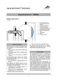
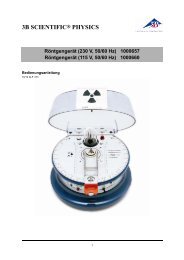
1 Anschlussbuchsen<br />
2 Rändelschraube zur Befestigung<br />
des Drehrahmens mit Flachspule<br />
3 <strong>Spulen</strong>paar<br />
4 Klemmfeder für Hallsonde<br />
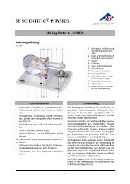
1. Beschreibung<br />
Die <strong>Helmholtz</strong>-<strong>Spulen</strong> dienen zur Erzeugung eines<br />
homogenen Magnetfeldes. Die <strong>Spulen</strong> ermöglichen<br />
Versuche zur Induktion und Schwebung in Verbindung<br />
mit dem Drehrahmen mit Flachspule<br />
(U8481510) sowie zur Bestimmung der spezifischen<br />
Ladung des Elektrons e/m mit der Fadenstrahlröhre<br />
(U8481420). Die <strong>Spulen</strong> können sowohl parallel als<br />
auch in Reihe geschaltet werden. Eine Klemmfeder<br />
am oberen Träger dient zur Halterung einer Hallsonde<br />
zur Messung des magnetischen Felds.<br />
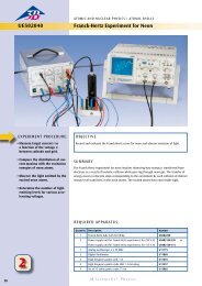
2. Technische Daten<br />
Windungszahl je Spule: 124<br />
<strong>Spulen</strong>durchmesser außen: 311 mm<br />
<strong>Spulen</strong>durchmesser innen: 287 mm<br />
Mittlerer <strong>Spulen</strong>radius:<br />
150 mm<br />
<strong>Spulen</strong>abstand:<br />
150 mm<br />
Kupferlackdrahtdicke:<br />
1,5 mm<br />
Gleichstromwiderstand:<br />
je 1,2 Ohm<br />
Max. <strong>Spulen</strong>strom:<br />
5 A<br />
Max. <strong>Spulen</strong>spannung:<br />
6 V<br />
Max. Flussdichte bei 5 A:<br />
3,7 mT<br />
Masse:<br />
ca. 4,1 kg<br />
1
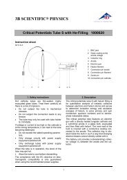
3. Theoretische Grundlagen<br />
Die <strong>Spulen</strong>anordnung geht auf den Physiker<br />
Hermann von <strong>Helmholtz</strong> zurück: Zwei kurze <strong>Spulen</strong><br />
mit großem Radius R werden im Abstand R auf gleicher<br />
Achse parallel aufgestellt. Das Feld jeder einzelnen<br />
Spule ist inhomogen. Durch die Überlagerung<br />
beider Felder ergibt sich zwischen beiden <strong>Spulen</strong> ein<br />
Bereich mit weitgehend homogenem Magnetfeld.<br />
Für die magnetische Flussdichte B des Magnetfeldes<br />
bei <strong>Helmholtz</strong>geometrie des <strong>Spulen</strong>paars und dem<br />
<strong>Spulen</strong>strom I gilt:<br />
3<br />
2<br />
⎛ 4 ⎞<br />
B = ⎜ ⎟ ⋅μ 0<br />
⎝ 5 ⎠<br />
n<br />
⋅I<br />
⋅<br />
R<br />
mit n = Windungsanzahl einer Spule, R = mittlerer<br />
<strong>Spulen</strong>radius und μ 0<br />
= magnetische Feldkonstante.<br />
Für die <strong>Helmholtz</strong>-<strong>Spulen</strong> ergibt sich:<br />
−4<br />
B = 7 , 433⋅10<br />
⋅I<br />
in Tesla (I in A).<br />
4. Versuchsbeispiele<br />
Zur Durchführung der Experimente werden folgenden<br />
Geräte zusätzlich benötigt:<br />
1 AC/DC Netzgerät 0–20 V, 5 A U8521131<br />
2 Multimeter Escola 10 U8531160<br />
1 Drehrahmen mit Flachspule U8481510<br />
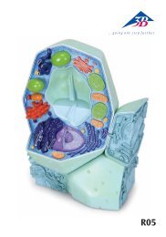
4.1 Spannungsinduktion im Magnetfeld<br />
• <strong>Helmholtz</strong>-<strong>Spulen</strong> auf der Tischplatte aufstellen<br />
und über ein Amperemeter mit der Gleichstromversorgung<br />
in Reihe schalten.<br />
• Den Drehrahmen mit der Flachspule mit seinen<br />
Trägern an den Querhalterungen der <strong>Helmholtz</strong>-<br />
<strong>Spulen</strong> festschrauben, so dass sich die Flachspule<br />
in der Mitte des homogenen Feldes der <strong>Helmholtz</strong>-<strong>Spulen</strong><br />
drehen lässt.<br />
• Voltmeter mit Nullpunkt Mitte direkt an die<br />
Flachspule anschließen.<br />
• Strom von ca. 1,5 A als Versorgung für die <strong>Spulen</strong><br />
einstellen.<br />
• Handkurbel betätigen und den Ausschlag im<br />
Voltmeter beobachten.<br />
• Drehgeschwindigkeit verändern, bis ein großer<br />
Ausschlag erreicht wird. Die Drehgeschwindigkeit<br />
muss niedrig sein.<br />
Zur Erreichung einer konstanten Drehgeschwindigkeit<br />
empfiehlt es sich den Drehrahmen über einen<br />
langsam drehenden Motor (z. B. Gleichstrommotor,<br />
12 V U8552330) anzutreiben.<br />
Der genaue Spannungsverlauf kann auch mit einem<br />
Oszilloskop beobachtet und gemessen werden.<br />
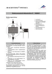
Fig. 1 <strong>Spulen</strong> in <strong>Helmholtz</strong>geometrie<br />
4.2. Bestimmung des Erdfeldes aus der Induktionsspannug<br />
Mit demselben Versuchsaufbau kann auch das magnetische<br />
Erdfeld gemessen werden.<br />
• <strong>Helmholtz</strong>spulen so ausrichten, dass die Magnetfelder<br />
der <strong>Helmholtz</strong>spule und der Erde parallel<br />
verlaufen<br />
• Flachspule drehen und Spannung beobachten.<br />
• Strom an der <strong>Helmholtz</strong>spule hoch drehen bis<br />
keine Induktionsspannung an den Ausgängen<br />
der Flachspule anliegt. (Kompensation des Erdmagnetfeldes<br />
durch das Feld der Helmoltzspule)<br />
Die Berechnung des Magnetfelds in den <strong>Spulen</strong>,<br />
wenn der induzierte Strom gleich Null ist, ergibt die<br />
Größe des Erdmagnetfelds.<br />
2
-<br />
0-12 V<br />
+<br />
V<br />
-<br />
+<br />
A<br />
0-30 V<br />
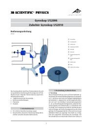
Fig. 2 Experimentieraufbau Drehrahmen mit Flachspule und Antriebsmotor<br />
Elwe Didactic GmbH • Steinfelsstr. 6 • 08248 Klingenthal • Deutschland • www.elwedidactic.com<br />
<strong>3B</strong> <strong>Scientific</strong> GmbH • Rudorffweg 8 • 21031 Hamburg • Deutschland • www.3bscientific.com<br />
Technische Änderungen vorbehalten
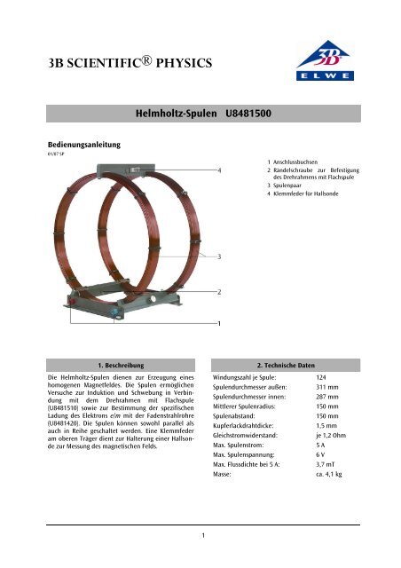
<strong>3B</strong> SCIENTIFIC® PHYSICS<br />
Pair of <strong>Helmholtz</strong> Coils <strong>U8481500</strong><br />
Instruction sheet<br />
01/07 SP<br />
1 Connection sockets<br />
2 Knurled screw for mounting the<br />
rotating frame with flat coil<br />
3 Pair of coils<br />
4 Spring clip for Hall sensor<br />
1. Description<br />
The Pair of <strong>Helmholtz</strong> coils is used for generating a<br />
homogeneous magnetic field. In conjunction with<br />
the rotating frame with flat coil (U8481510), the<br />
<strong>Helmholtz</strong> coils are also used in experiments for<br />
investigating induction and magnetic levitation. and<br />
for the determination of the specific charge of the<br />
electron e/m in conjunction with the electron-beam<br />
tube (U8481420). The coils can be switched in parallel<br />
or in series. A spring clip on the top crossbar is<br />
used to mount the Hall sensor during measurements<br />
of the magnetic field.<br />
2. Technical data<br />
Number of turns per coil: 124<br />
Outer coil diameter:<br />
311 mm<br />
Inner coil diameter:<br />
287 mm<br />
Mean coil radius:<br />
150 mm<br />
Coil spacing:<br />
150 mm<br />
Enamelled copper wire thickness: 1.5 mm<br />
DC resistance:<br />
1.2 Ohm each<br />
Maximum coil current:<br />
5 A<br />
Maximum coil voltage:<br />
6 V<br />
Maximum flux density at 5 A: 3.7 mT<br />
Weight:<br />
4.1 kg approx.<br />
1
3. Theoretical bases<br />
The special arrangement of the coils is attributed to<br />
the physicist Hermann von <strong>Helmholtz</strong>. Two narrow<br />
coils with a large radius R are set up parallel to one<br />
another and on the same axis so that they are also<br />
separated by a distance R. The magnetic field of each<br />
individual coil is non-uniform. Upon superimposition<br />
of the two fields, a region with a magnetic field that<br />
is largely uniform is created between the two coils.<br />
Given the <strong>Helmholtz</strong> arrangement of the pair of coils<br />
and coil current I, the following holds true for the<br />
magnetic flux density B of the magnetic field:<br />
3<br />
2<br />
⎛ 4 ⎞<br />
B = ⎜ ⎟ ⋅µ 0<br />
⎝ 5 ⎠<br />
n<br />
⋅I<br />
⋅<br />
R<br />
where n = number of turns in each coil, R = mean<br />
coil radius and µ 0<br />
= magnetic field constant.<br />
For the <strong>Helmholtz</strong> pair of coils, we get:<br />
−4<br />
B = 7 . 433⋅<br />
10 ⋅I<br />
in Tesla (I in A).<br />
Fig. 1 Coils in <strong>Helmholtz</strong> arrangement<br />
4. Sample experiments<br />
In order to perform the experiments,the following<br />
equipment is also required:<br />
1 AC/DC power supply 0-20 V, 5 A U8521131<br />
2 Escola 10 multimeter U8531160<br />
1 Rotating frame with flat coil U8481510<br />
4.1 Voltage induction in a magnetic field<br />
• Position the <strong>Helmholtz</strong> coils on the table top and<br />
connect them in series to the DC power supply<br />
via an ammeter.<br />
• Screw the supports of the rotating frame with the<br />
flat coil to the crossbar of the <strong>Helmholtz</strong> coils, so<br />
that the flat coil can rotate in the middle of the<br />
uniform field produced by the <strong>Helmholtz</strong> coils.<br />
• Connect a voltmeter with a central zero point<br />
directly across the coil.<br />
• Set the power supply current for the coils to<br />
about 1.5 A.<br />
• Use the hand crank and observe the deflection of<br />
the voltmeter.<br />
• Change the speed of rotation so that a larger<br />
deflection is obtained. The rotation speed needs<br />
to be low.<br />
In order to achieve a constant speed of rotation, use<br />
of a slowly rotating motor (e.g. 12 V DC motor<br />
U8552330) is recommended for driving the rotating<br />
frame.<br />
A precise voltage trace can also be observed and<br />
measured using an oscilloscope.<br />
4.2. Determination of the earth’s magnetic field<br />
from the induction voltage<br />
Using the same experiment set-up, it is also possible<br />
to measure the earth’s magnetic field.<br />
• Align the <strong>Helmholtz</strong> coils in such a way that the<br />
magnetic field of the coils is parallel to the<br />
Earth’s field.<br />
• Rotate the flat coil and observe the voltage.<br />
• Increase current to the <strong>Helmholtz</strong> coils until the<br />
voltage induced at the outputs of the flat coil is<br />
zero (so that the earth’s magnetic field and the<br />
field of the <strong>Helmholtz</strong> coils cancel out).<br />
• When the induced current is 0, then the magnetic<br />
field in the coils is of the same magnitude<br />
as the Earth’s magnetic field.<br />
2
-<br />
0-12 V<br />
+<br />
V<br />
-<br />
+<br />
A<br />
0-30 V<br />
Fig. 2 Experiment set-up with flat coil and driving motor<br />
Elwe Didactic GmbH • Steinfelsstr. 6 • 08248 Klingenthal • Germany • www.elwedidactic.com<br />
<strong>3B</strong> <strong>Scientific</strong> GmbH • Rudorffweg 8 • 21031 Hamburg • Germany • www.3bscientific.com<br />
Subject to technical amendments
<strong>3B</strong> SCIENTIFIC® PHYSICS<br />
Paire de bobines de <strong>Helmholtz</strong> <strong>U8481500</strong><br />
Instructions d’utilisation<br />
01/07 SP<br />
1 Douilles de sortie<br />
2 Vis moletée pour fixer le cadre<br />
rotatif avec bobine plate<br />
3 Bobines de <strong>Helmholtz</strong><br />
4 Ressort disposé pour sonde de Hall<br />
1. Description<br />
La paire de bobines de <strong>Helmholtz</strong> sert à générer un<br />
champ magnétique homogène. Les bobines permettent<br />
de réaliser des expériences sur l'induction et le<br />
battement en liaison avec le cadre tournant à bobine<br />
plate (U8481510) et pour la détermination de la<br />
charge spécifique e/m de l'électron avec le tube à<br />
pinceau étroit (U8481420). Les bobines peuvent être<br />
montées en parallèle ou en série. Un ressort disposé<br />
sur la traverse supérieure permet de fixer une sonde<br />
de Hall lors de la détermination du champ magnétique.<br />
2. Caractéristiques techniques<br />
Spires par bobine: 124<br />
Diamètre de bobine ext.:<br />
311 mm<br />
Diamètre de bobine int.:<br />
287 mm<br />
Rayon de bobine moyen:<br />
150 mm<br />
Ecart de bobines:<br />
150 mm<br />
Epaisseur de fil en<br />
cuivre émaillé:<br />
1,5 mm<br />
Résistance du courant<br />
continu:<br />
1,2 Ohm chacune<br />
Courant de bobine max.:<br />
5 A<br />
Tension de bobine max.:<br />
6 V<br />
Densité de flux max. à 5 A:<br />
3,7 mT<br />
Masse:<br />
env. 4,1 kg<br />
1
3. Notions théoriques<br />
L'agencement des bobines est le résultat d'études<br />
réalisées par le physicien Hermann von <strong>Helmholtz</strong> :<br />
deux bobines courtes de rayon R sont placées parallèlement<br />
sur un même axe dans un écart R. Le<br />
champ de chaque bobine est inhomogène. Par la<br />
superposition des deux champs, on obtient entre les<br />
deux bobines une zone présentant un champ magnétique<br />
pratiquement homogène.<br />
L'équation suivante s'applique à la densité de flux<br />
magnétique B dans le cas d'une géométrie <strong>Helmholtz</strong><br />
du champ magnétique de la paire de bobines et d'un<br />
courant de bobines I:<br />
3<br />
2<br />
⎛ 4 ⎞<br />
B = ⎜ ⎟ ⋅µ 0<br />
⎝ 5 ⎠<br />
n<br />
⋅I<br />
⋅<br />
R<br />
n = nombre de spires d'une bobine, R = rayon de<br />
bobine moyen et µ 0<br />
= constante de champ magnétique.<br />
Pour la paire de bobines <strong>Helmholtz</strong>, on obtient:<br />
−4<br />
B = 7 , 433⋅10<br />
⋅I<br />
en teslas (I en A).<br />
Fig. 1 Bobines dans la géométrie <strong>Helmholtz</strong><br />
4. Exemples d'expériences<br />
Pour réaliser les expériences, vous nécessitez le matériel<br />
supplémentaire suivant :<br />
1 alimentation CA/CC 0–20 V, 5 A U8521131<br />
2 multimètres Escola 10 U8531160<br />
1 cadre rotatif à bobine plate U8481510<br />
4.1 Induction de tension dans le champ magnétique<br />
• Placez les bobines de <strong>Helmholtz</strong> sur la plaque et<br />
montez-les en série avec l'alimentation en tension<br />
continue en vous servant d'un ampèremètre.<br />
• Vissez le cadre rotatif avec la bobine plate et ses<br />
supports aux fixations transversales des bobines<br />
de <strong>Helmholtz</strong>, de manière à ce que la bobine<br />
plate puisse être tournée au centre du champ<br />
homogène des bobines <strong>Helmholtz</strong>.<br />
• Branchez le voltmètre à point zéro central directement<br />
à la bobine plate.<br />
• Réglez un courant d'alimentation d'environ 1,5 A<br />
pour les bobines.<br />
• Actionnez la manivelle et observez la déviation<br />
sur le voltmètre.<br />
• Modifiez la vitesse de rotation, jusqu'à ce que<br />
vous obteniez une forte déviation. La vitesse de<br />
rotation doit être faible.<br />
Pour obtenir une vitesse de rotation constante, il est<br />
recommandé d'entraîner le cadre tournant avec un<br />
moteur lent (par ex. moteur à courant continu 12 V,<br />
U8552330).<br />
L'allure de la tension peut être observée et mesurée<br />
avec précision à l'aide d'un oscilloscope.<br />
4.2. Détermination du champ terrestre à partir de<br />
la tension d'induction<br />
Le même montage permet de mesurer le champ<br />
magnétique terrestre.<br />
• Ajustez les bobines <strong>Helmholtz</strong> de manière à ce<br />
que les champs magnétiques de la bobine soient<br />
parallèles à la terre.<br />
• Tournez la bobine plate et observez la tension.<br />
• Augmentez le courant au niveau de la bobine de<br />
<strong>Helmholtz</strong>, jusqu'à ce que les sorties de la bobine<br />
plate soient exemptes de tension d'induction<br />
(compensation du champ magnétique terrestre<br />
par le champ de la bobine de <strong>Helmholtz</strong>).<br />
Le calcul du champ magnétique dans les bobines,<br />
lorsque le courant induit est nul, donne la grandeur<br />
du champ magnétique terrestre.<br />
2
-<br />
0-12 V<br />
+<br />
V<br />
-<br />
+<br />
A<br />
0-30 V<br />
Fig. 2 Cadre rotatif avec bobine plate et moteur d'entraînement<br />
Elwe Didactic GmbH • Steinfelsstrasse 6 • 08248 Klingenthal • Allemagne • www.elwedidactic.com<br />
<strong>3B</strong> <strong>Scientific</strong> GmbH • Rudorffweg 8 • 21031 Hambourg • Allemagne • www.3bscientific.com<br />
Sous réserve de modifications techniques
<strong>3B</strong> SCIENTIFIC® PHYSICS<br />
Coppia di bobine di <strong>Helmholtz</strong> <strong>U8481500</strong><br />
Istruzioni per l'uso<br />
01/07 SP<br />
1 Presa di uscita<br />
2 Vite a testa zigrinata per il fissaggio<br />
del telaio rotante con bobina<br />
piatta<br />
3 Bobine di <strong>Helmholtz</strong><br />
4 Molla di serraggio per sonda di Hall<br />
1. Descrizione<br />
La coppia di bobine di <strong>Helmholtz</strong> serve per generare<br />
un campo magnetico omogeneo. Le bobine consentono<br />
prove sull’induzione e sul battimento in combinazione<br />
con il telaio rotante con bobina piatta<br />
(U8481510) così come per la determinazione della<br />
carica specifica e/m dell'elettrone con il tubo a fascio<br />
elettronico (U8481420). Le bobine possono essere<br />
collegate in parallelo o in serie. Una molla di serraggio<br />
presente sul raccordo trasversale superiore rende<br />
possibile il bloccaggio di una sonda di Hall durante la<br />
determinazione del campo magnetico.<br />
2. Dati tecnici<br />
Numero di spire per bobina: 124<br />
Diametro esterno bobina: 311 mm<br />
Diametro interno bobina: 287 mm<br />
Raggio centrale bobina:<br />
150 mm<br />
Distanza bobine:<br />
150 mm<br />
Spessore filo di rame smaltato: 1,5 mm<br />
Resistenza ohmica:<br />
ogni 1,2 Ohm<br />
Corrente bobina max.:<br />
5 A<br />
Tensione bobina max.:<br />
6 V<br />
Densità flusso max. a 5 A:<br />
3,7 mT<br />
Peso:<br />
ca. 4,1 kg<br />
1
3. Principi teorici<br />
La disposizione delle bobine risale al fisico Hermann<br />
von <strong>Helmholtz</strong>: due bobine corte con ampio raggio R<br />
vengono posizionate parallelamente sullo stesso asse<br />
alla distanza R. Il campo di ogni singola bobina non<br />
è omogeneo. Attraverso la sovrapposizione dei due<br />
campi, tra le due bobine si ottiene un’area con<br />
campo magnetico ampiamente omogeneo.<br />
Per la densità di flusso magnetica B del campo magnetico<br />
secondo la geometria di <strong>Helmholtz</strong> della copia<br />
di bobine e della corrente di bobina I vale quanto<br />
segue:<br />
3<br />
2<br />
⎛ 4 ⎞<br />
B = ⎜ ⎟ ⋅µ 0<br />
⎝ 5 ⎠<br />
n<br />
⋅I<br />
⋅<br />
R<br />
in cui n = numero di spire di una bobina, R = raggio<br />
centrale della bobina e µ 0<br />
= costante di campo magnetico.<br />
Per la coppia di bobine di <strong>Helmholtz</strong> si ottiene:<br />
−4<br />
B = 7 , 433⋅10<br />
⋅I<br />
in Tesla (I in A)<br />
Fig. 1 Bobine nella geometria di <strong>Helmholtz</strong><br />
4. Esempi di esperimenti<br />
Per l’esecuzione degli esperimenti sono necessari i<br />
seguenti apparecchi:<br />
1 alimentatore CA/CC 0–20 V, 5 A U8521131<br />
2 multimetri Escola 10 U8531160<br />
1 telaio rotante con bobina piatta U8481510<br />
4.1 Induzione della tensione nel campo magnetico<br />
• Collocare le bobine di <strong>Helmholtz</strong> sul piano del<br />
tavolo e attraverso un amperometro collegarle in<br />
serie con alimentazione di corrente continua.<br />
• Avvitare il telaio rotante con bobina piatta e i<br />
supporti ai raccordi trasversali delle bobine di<br />
<strong>Helmholtz</strong> in modo da potere far ruotare la bobina<br />
piatta al centro del campo omogeneo delle<br />
bobine di <strong>Helmholtz</strong>.<br />
• Collegare il voltmetro con punto zero centro<br />
direttamente alla bobina piatta.<br />
• Impostare una corrente di alimentazione delle<br />
bobine di circa 1,5 A.<br />
• Attivare la manovella e osservare l’oscillazione<br />
del voltmetro.<br />
• Modificare la velocità di rotazione fino a raggiungere<br />
un’oscillazione maggiore. La velocità di<br />
rotazione deve essere bassa.<br />
Per ottenere una velocità di rotazione costante, è<br />
consigliabile azionare il telaio rotante tramite un<br />
motore a rotazione lenta (ad es. motore a corrente<br />
continua, 12 V U8552330).<br />
L’andamento esatto della tensione può essere osservato<br />
e misurato anche mediante un oscilloscopio.<br />
4.2. Determinazione del campo terrestre dalla<br />
tensione d’induzione<br />
Con la stessa struttura di prova è possibile misurare<br />
anche il campo magnetico terrestre.<br />
• Allineare le bobine di <strong>Helmholtz</strong> in modo che i<br />
campi magnetici della bobina di <strong>Helmholtz</strong> e la<br />
terra siano paralleli.<br />
• Ruotare la bobina piatta e osservare la tensione.<br />
• Aumentare la corrente in corrispondenza della<br />
bobina di <strong>Helmholtz</strong> finché non è più presente<br />
nessuna tensione d’induzione alle uscite della<br />
bobina piatta. (Compensazione del campo magnetico<br />
terrestre attraverso il campo della bobina<br />
di <strong>Helmholtz</strong>)<br />
Il calcolo del campo magnetico nelle bobine, quando<br />
la corrente indotta è pari a zero, fornisce le dimensioni<br />
del campo magnetico terrestre.<br />
2
-<br />
0-12 V<br />
+<br />
V<br />
-<br />
+<br />
A<br />
0-30 V<br />
Fig. 2 Struttura di prova telaio rotante con bobina piatta e motore di azionamento<br />
Elwe Didactic GmbH • Steinfelsstr. 6 • 08248 Klingenthal • Germania • www.elwedidactic.com<br />
<strong>3B</strong> <strong>Scientific</strong> GmbH • Rudorffweg 8 • 21031 Amburgo • Germania • www.3bscientific.com<br />
Con riserva di modifiche tecniche
<strong>3B</strong> SCIENTIFIC® PHYSICS<br />
Par de bobinas de <strong>Helmholtz</strong> <strong>U8481500</strong><br />
Instrucciones de uso<br />
01/07 SP<br />
1 Casquillos de conexión<br />
2 Tornillo moleteado para fijar el<br />
marco giratorio con la bobina<br />
plana<br />
3 Par de bobinas<br />
4 Muelle de borna para la sonda de<br />
Hall<br />
1. Descripción<br />
El par de bobinas de <strong>Helmholtz</strong> sirve para la producción<br />
de un campo magnético homogéneo. Las bobinas<br />
hacen posible la realización de experimentos<br />
sobre inducción y batidos con el marco giratorio con<br />
bobina plana (U8481510), así como para<br />
determinación de la carga específica e/m del electrón<br />
con el tubo de haz fino (U8481420). Las bobinas se<br />
pueden conectar en serie o en paralelo. Un muelle<br />
de apriete, ubicado en la parte superior del<br />
travesaño, sirve para la sujeción de una sonda de<br />
efecto Hall durante la determinación del campo<br />
magnético.<br />
2. Datos técnicos<br />
Número de espiras de cada bobina: 124<br />
Diametro externo de las bobinas: 311 mm<br />
Diametro interno de las bibonas: 287 mm<br />
Radio medio de las bobinas: 150 mm<br />
Distancia entre bobinas:<br />
150 mm<br />
Espesor del alambre de<br />
cobre esmaltado:<br />
1,5 mm<br />
Resistencia de corriente continua: cada 1,2 Ohm<br />
Máx. corriente de bobina: 5 A<br />
Máx. tensión de bobina:<br />
6 V<br />
Máx. densidad de flujo con 5 A: 3,7 mT<br />
Peso:<br />
aprox. 4,1 kg<br />
1
3. Fundamentos teóricos<br />
Esta Ordenación de las bobinas data del físico<br />
Hermann von <strong>Helmholtz</strong>. Dos bobinas cortas de un<br />
radio grande R se colocan paralelamente una frente<br />
a la otra en un mismo eje a una distancia R. El<br />
campo de cada una de ellas es inhomogéneo. Por la<br />
superposición de los campos en la región entre las<br />
bobinas se origina un campo magnético ámpliamente<br />
homogéneo..<br />
Para la densidad de campo magnético B del campo<br />
magnético en la geometría de <strong>Helmholtz</strong> del par de<br />
bobinas con una corriente I por las bobinas se tiene:<br />
3<br />
2<br />
⎛ 4 ⎞<br />
B = ⎜ ⎟ ⋅µ 0<br />
⎝ 5 ⎠<br />
n<br />
⋅I<br />
⋅<br />
R<br />
siendo n = el número de espiras de una bobina, R =<br />
radio medio de la bobina y µ 0<br />
= constante de campo<br />
magnético:<br />
−4<br />
B = 7 , 433⋅10<br />
⋅I<br />
en Tesla (I en A).<br />
Fig. 1 Bobinas en geometría de <strong>Helmholtz</strong><br />
4. Ejemplos de experimentos<br />
Para la realización de los experimentos se requieren<br />
los siguientes aparatos:<br />
1 Fuente CA/CC 0–20 V, 5 A U8521131<br />
2 Multímetros Escola 10 U8531160<br />
1 Marco giratorio con bobina plana U8481510<br />
4.1 Inducción de tensión en el campo magnético<br />
• Se colocan las bobinas de <strong>Helmholtz</strong> sobre la<br />
mesa de trabajo y se conectan serie entre sí y<br />
luego en serie con un amperímetro y con la<br />
fuente de alimentación de tensión continua.<br />
• El marco giratorio con la bobina plana con sus<br />
soportes se fija con los tornillos moleteados en<br />
los travesaños distanciadores de las bobinas de<br />
<strong>Helmholtz</strong>, de tal forma que ésta se pueda girar<br />
en el centro del campo homogéneo de las<br />
bobinas de <strong>Helmholtz</strong>.<br />
• Se conecta el voltímetro directamente en los<br />
contactos de la bobina plana.<br />
• Se ajusta la corriente en aprox. 1,5 A como<br />
suministro de las bobinas de <strong>Helmholtz</strong>.<br />
• Se acciona la manivela con la mano y se observa<br />
la señal en el voltímetro.<br />
• Se varía la velocidad de rotación de la bobina<br />
hasta que se obtenga la máxima señal en<br />
voltímetro. La velocidad de rotación debe ser<br />
lenta.<br />
Para lograr un velocidad de rotación constante se<br />
recomienda accionar el marco giratorio por medio de<br />
un motor de revoluciones lentas (p.ej.: Motor de<br />
corriente continua, 12 V U8552330).<br />
El curso exacto de la tensión inducida se puede<br />
observar y medir por medio de un osciloscopio.<br />
4.2. Determinación del campo magnético terrestre<br />
por medio de la tensión inducida<br />
Con el mismo montaje experimental del punto 5.1 se<br />
puede medir el campo magnético terrestre.<br />
• Se orientan las bobinas de <strong>Helmholtz</strong> de tal<br />
forma que el campo magnético originado por las<br />
bobinas de <strong>Helmholtz</strong> sea antiparalelo al campo<br />
magnético terrestre.<br />
• Se hace rotar la bobina plana y se observa la<br />
tensión de inducción en el voltímetro.<br />
• Se varía la corriente en las bobinas de <strong>Helmholtz</strong><br />
hasta que en la salida de la bobina plana la<br />
tensión de inducción llegue a cero<br />
(Compensación del campo magnético terrestre<br />
por el campo magnético de las bobinas de<br />
<strong>Helmholtz</strong>).<br />
El cálculo del campo magnético en la geometría de<br />
<strong>Helmholtz</strong> cuando la corriente inducida sea cero da<br />
por resultado la intensidad del campo magnético<br />
terrestre.<br />
2
-<br />
0-12 V<br />
+<br />
V<br />
-<br />
+<br />
A<br />
0-30 V<br />
Fig. 2 Montaje experimental del marco giratorio con bobina plana y motor de accionamiento<br />
Elwe Didactic GmbH • Steinfelsstr. 6 • 08248 Klingenthal • Deutschland • www.elwedidactic.com<br />
<strong>3B</strong> <strong>Scientific</strong> GmbH • Rudorffweg 8 • 21031 Hamburg • Deutschland • www.3bscientific.com<br />
Se reservan las modificaciones técnicas
<strong>3B</strong> SCIENTIFIC® PHYSICS<br />
Par de bobinas de <strong>Helmholtz</strong> <strong>U8481500</strong><br />
Instruções para o uso<br />
01/07 SP<br />
1 Conectores saída<br />
2 Parafuso manual para a fixação do<br />
quadro rotativo com bobina plana<br />
3 Bobinas <strong>Helmholtz</strong><br />
4 Pinça de fixação para fixar uma<br />
sonda Hall<br />
1. Descrição<br />
As bobinas de <strong>Helmholtz</strong> servem para a produção de<br />
campos magnéticos homogêneos. As bobinas<br />
permitem experiências com a indução e a flutuação<br />
associadas ao quadro giratório com bobina plana<br />
(U8481510) para a determinação da carga específica<br />
e/m do elétron o tubo de raio linear (U8481420). As<br />
bobinas podem ser conectadas tanto em paralelo<br />
como em série. A pinça de fixação que está na barra<br />
transversal superior, serve para fixar uma sonda Hall<br />
quando o campo magnético para determinação.<br />
2. Dados técnicos<br />
Espiras por bobina: 124<br />
Diâmetro externo da bobina: 311 mm<br />
Diâmetro interno da bobina: 287 mm<br />
Rádio médio da bobina:<br />
150 mm<br />
Distância entre as bobinas:<br />
150 mm<br />
Espessura do fio de cobre laqueado: 1,5 mm<br />
Resistência de corrente contínua: 1,2 Ohm cada<br />
Corrente máx. bobina:<br />
5 A<br />
Tensão máx. bobina:<br />
6 V<br />
Densidade de corrente máx. a 5 A: 3,7 mT<br />
Massa:<br />
aprox. 4,1 kg<br />
1
3. Fundamentos teóricos<br />
A ordenação das bobinas foi elaborada pelo físico<br />
Hermann von <strong>Helmholtz</strong>: duas bobinas curtas com<br />
rádio maior R são colocadas em paralelo ao mesmo<br />
eixo com distância R entre si. O capo produzido por<br />
cada bobina não é homogêneo. Através da<br />
superposição dos campos de ambas bobinas resulta<br />
então um campo magnético praticamente<br />
homogêneo entre as duas bobinas.<br />
Para a densidade de fluxo magnético B do campo<br />
magnético dentro da geometria de <strong>Helmholtz</strong> do par<br />
de bobinas e a corrente de bobina I é válido:<br />
3<br />
2<br />
⎛ 4 ⎞<br />
B = ⎜ ⎟ ⋅µ 0<br />
⎝ 5 ⎠<br />
n<br />
⋅I<br />
⋅<br />
R<br />
com n = número de espiras de uma bobina, R =<br />
rádio médio da bobina e µ 0<br />
= constante de campo<br />
magnético.<br />
Para o par de bobinas de <strong>Helmholtz</strong> resulta:<br />
−4<br />
B = 7 , 433⋅10<br />
⋅I<br />
em Tesla (I em A).<br />
Fig. 1 Bobinas em geometria de <strong>Helmholtz</strong><br />
4. Exemplos de experiências<br />
Para a execução das experiências são necessários os<br />
seguintes aparelhos:<br />
1 Aparelho de alim. AC/DC 0–20 V, 5 A U8521131<br />
2 Multímetro Escola 10 U8531160<br />
1 Quadro rotativo com bobina plana U8481510<br />
4.1 Indução de tensão em campos magnéticos<br />
• Colocar as bobinas de <strong>Helmholtz</strong> sobre a mesa<br />
de trabalho e conecta-las em série com a<br />
alimentação em corrente contínua passando por<br />
um amperímetro.<br />
• Aparafusar firmemente o quadro rotativo com a<br />
bobina plana e seus suportes nos apoios<br />
perpendiculares das bobinas de <strong>Helmholtz</strong>, de<br />
modo que a bobina plana possa ser girada no<br />
meio do campo homogêneo das bobinas de<br />
<strong>Helmholtz</strong>.<br />
• Ligar o voltímetro com ponto zero mediano<br />
diretamente com a bobina plana.<br />
• Ajustar uma corrente de alimentação de<br />
aproximadamente 1,5 A como alimentação para<br />
as bobinas.<br />
• Acionar a manivela e observar os valores no<br />
voltímetro.<br />
• Alterar a velocidade de rotação até que se atinja<br />
um valor maior. A velocidade de rotação deve ser<br />
baixa.<br />
Para se alcançar uma velocidade de rotação<br />
constante, recomenda-se proporcionar um motor de<br />
rotação lenta para impulsar o quadro giratório (por<br />
exemplo, motor de corrente contínua, 12 V<br />
U8552330).<br />
A evolução exata da tensão pode ser observada e<br />
medida com a ajuda de um osciloscópio.<br />
4.2. Determinação do campo terrestre a partir da<br />
tensão de indução<br />
Com a mesma montagem da experiência pode-se<br />
também medir o campo magnético da Terra.<br />
• Instalar as bobinas de <strong>Helmholtz</strong> de modo que o<br />
campo magnético das bobinas de <strong>Helmholtz</strong> e o<br />
campo magnético da Terra estejam em paralelo.<br />
• Girar a bobina plana e observar a tensão.<br />
• Elevar a corrente nas bobinas de <strong>Helmholtz</strong> até<br />
que não há nenhuma tensão de indução nas<br />
saídas da bobina plana (compensação do campo<br />
magnético terrestre através do campo da bobina<br />
de Helmoltz)<br />
O cálculo do campo magnético das bobinas quando a<br />
corrente induzida é igual a zero resulta no tamanho<br />
do campo magnético.<br />
2
-<br />
0-12 V<br />
+<br />
V<br />
-<br />
+<br />
A<br />
0-30 V<br />
Fig. 2 montagem da experiência com o quadro rotativo com bobina plana e motor de impulso<br />
Elwe Didactic GmbH • Steinfelsstr. 6 • 08248 Klingenthal • Alemanha • www.elwedidactic.com<br />
<strong>3B</strong> <strong>Scientific</strong> GmbH • Rudorffweg 8 • 21031 Hamburgo • Alemanha • www.3bscientific.com<br />
Sob reserva de alterações técnicas