Mechanics - 3B Scientific
Mechanics - 3B Scientific
Mechanics - 3B Scientific

Create successful ePaper yourself
Turn your PDF publications into a flip-book with our unique Google optimized e-Paper software.
<strong>Mechanics</strong><br />
Oscillations<br />
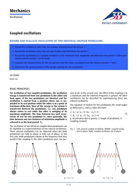
Coupled oscillations<br />
RECORD AND EVALUATE OSCILLATION OF TWO IDENTICAL COUPLED PENDULUMS.<br />
• Record the oscillations when they are in phase and determine the period T +<br />
.<br />
• Record the oscillations when they are out of phase and determine the period T –<br />
.<br />
• Record the oscillations of a coupled pendulum at the maximum beat amplitude and determine the period T of the oscillations<br />
and the period T ∆ of the beats.<br />
• Compare the measurements for the two periods with the values calculated from the intrinsic periods T –<br />
and T +<br />
.<br />
• Determine the spring constant of the spring coupling the two pendulums.<br />
UE105060<br />
04/07 CW<br />
BASIC PRINCIPLES<br />
For oscillation of two coupled pendulums, the oscillation<br />
energy is transferred from one pendulum to the other and<br />
back again. If the two pendulums are identical and the<br />
oscillation is started from a position where one is suspended<br />
in its rest position while the other is at a point of<br />
maximum deflection, then all the energy in the system is<br />
transferred between the pendulums. I.e. one pendulum<br />
always comes to rest while the other is swinging at its<br />
maximum amplitude. The time between two such occurrences<br />
of rest for one pendulum or, more generally, the<br />
time between any two instances of minimum amplitude is<br />
referred to as the beat period. T ∆ .<br />
The oscillation of two identical coupled ideal pendulums can<br />
be regarded as a superimposition of two natural oscillations.<br />
These natural oscillations can be observed when the both<br />
pendulums are fully in phase or fully out of phase. In the<br />
first case, both pendulums vibrate at the frequency that they<br />
would if the coupling to the other pendulum were not present<br />
at all. In the second case, the effect of the coupling is at<br />
a maximum and the inherent frequency is greater. All other<br />
oscillations can be described by superimposing these two<br />
natural oscillations.<br />
The equation of motion for the pendulums (for small angles<br />
of deflection ϕ 1 and ϕ 2 ) takes the form:<br />
⋅ ( ϕ1<br />
− ϕ2<br />
) = 0<br />
⋅ ( ϕ − ϕ ) = 0<br />
L ⋅ ϕ&&<br />
1 + g ⋅ ϕ1<br />
+ k<br />
L ⋅ ϕ&&<br />
2 + g ⋅ ϕ2<br />
+ k 2 1<br />
g: Acceleration due to gravity, L: length of pendulum, k:<br />
coupling constant<br />
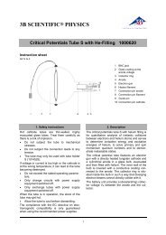
Fig. 1: Left: general coupled oscillation, Middle: coupled oscillation<br />
in phase, Right: coupled oscillation out of phase<br />
(1)<br />
ϕ 1 ϕ 2 ϕ<br />
ϕ ϕ ϕ<br />
ϕ<br />
−ϕ<br />
ϕ<br />
1 = 2 =<br />
- ϕ1 = ϕ2= ϕ<br />
1 / 5
UE105060<br />
<strong>3B</strong> SCIENTIFIC® PHYSICS EXPERIMENT<br />
For the motions ϕ + = ϕ1 + ϕ2<br />
and ϕ − = ϕ1 − ϕ2<br />
(initially<br />
chosen arbitrarily) the equation of motion is as follows:<br />
L ⋅ ϕ&&<br />
L ⋅ ϕ&&<br />
+<br />
−<br />
+ g ⋅ ϕ<br />
+<br />
+<br />
The solutions<br />
ϕ<br />
ϕ<br />
+<br />
−<br />
= 0<br />
( g + 2k) ⋅ ϕ = 0<br />
= a cos<br />
+<br />
= a cos<br />
−<br />
−<br />
( ω+<br />
t) + b+<br />
sin( ω+<br />
t)<br />
( ω t) + b sin( ω t)<br />
−<br />
give rise to angular frequencies<br />
−<br />
−<br />
g<br />
g + 2k<br />
ω + = und ω − =<br />
(4)<br />
L<br />
L<br />
corresponding to the natural frequencies for in phase or out<br />
of phase motion (ϕ +<br />
= 0 for out of phase motion and ϕ –<br />
= 0<br />
for in-phase motion).<br />
The deflection of the pendulums can be calculated from the<br />
sum or the difference of the two motions, leading to the<br />
solutions<br />
1<br />
ϕ1<br />
=<br />
2<br />
1<br />
ϕ2<br />
=<br />
2<br />
( a cos( ω t) + b sin( ω t) + a cos( ω t) + b sin( ω t)<br />
)<br />
+<br />
( a cos( ω t) + b sin( ω t) − a cos( ω t) − b sin( ω t)<br />
)<br />
+<br />
+<br />
+<br />
+<br />
+<br />
+<br />
+<br />
Parameters a +<br />
, a –<br />
, b +<br />
and b –<br />
are arbitrary coefficients that<br />
can be calculated from the initial conditions for the two<br />
pendulums at time t = 0.<br />
The easiest case to interpret is where pendulum 1 is deflected<br />
by an angle ϕ 0 from its rest position and released at<br />
time 0 while pendulum 2 remains in its rest position.<br />
1<br />
ϕ1<br />
= ⋅<br />
2<br />
1<br />
ϕ2<br />
= ⋅<br />
2<br />
( ϕ ⋅ cos( ω t) + ϕ ⋅cos( ω t)<br />
)<br />
0<br />
+<br />
( ϕ ⋅ cos( ω t) − ϕ ⋅ cos( ω t)<br />
)<br />
0<br />
+<br />
0<br />
After rearranging the equations they take the form<br />
ϕ1<br />
= ϕ0<br />
⋅ cos<br />
ϕ = ϕ ⋅ sin<br />
2<br />
with<br />
0<br />
ω−<br />
− ω<br />
ω∆<br />
=<br />
2<br />
ω+<br />
+ ω−<br />
ω =<br />
2<br />
0<br />
( ω∆t) ⋅cos( ωt)<br />
( ω t) ⋅cos( ωt)<br />
+<br />
∆<br />
This corresponds to an oscillation of both pendulums at<br />
identical angular frequency ω, where the amplitudes are<br />
modulated at an angular frequency ω ∆ . This kind of modulation<br />
results in beats. In the situation described, the amplitude<br />
of the beats arrives at a maximum since the overall<br />
amplitude falls to a minimum at zero.<br />
−<br />
−<br />
−<br />
−<br />
−<br />
−<br />
−<br />
−<br />
−<br />
−<br />
(2)<br />
(3)<br />
(5)<br />
(6)<br />
(7)<br />
(8)<br />
LIST OF APPARATUS<br />
2 Pendulum rods with angle sensor U8404270<br />
1 Transformer 12 V, 2 A, e.g. U8475430<br />
1 Helical spring with two eyelets, 3 N/m U15027<br />
2 Table clamps U13260<br />
2 Stainless steel rods, 1000 mm U15004<br />
1 Stainless steel rod, 470 mm U15002<br />
4 Universal clamps U13255<br />
1 <strong>3B</strong> NETlog U11300<br />
1 <strong>3B</strong> NETlab for Windows U11310<br />
1 PC with Windows 98/2000/XP, Internet Explorer 6 or later,<br />
USB port<br />
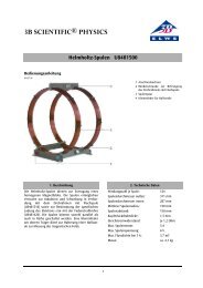
SET-UP<br />
Fig. 2<br />
Set-up for recording and evaluating the oscillation of two<br />
identical pendulums coupled together by a spring<br />
The set-up is illustrated in Fig. 2.<br />
• Clamp two stand rods of 1000 mm length to a bench so<br />
that they are about 15 cm apart.<br />
• Attach a short stand rod between them as a horizontal<br />
cross member to lend the set-up more stability.<br />
• Attach the angle sensors to the top of the vertical rods<br />
using universal clamps.<br />
• Attach bobs to the end of the pendulum rods.<br />
• Suspend the pendulum rods from the angle sensors<br />
(there are grooves in the angle sensors to accommodate<br />
the hinge pins of the pendulum rods)<br />
2 / 5
UE105060<br />
<strong>3B</strong> SCIENTIFIC® PHYSICS EXPERIMENT<br />
• Attach the spring via the holes in the pendulum rods.<br />
These are about 40 cm from the fulcrum of the pendulum.<br />
• Attach the angle sensor by means of cables to a transformer.<br />
Make sure to use the cables labelled 12 V.<br />
• Connect the <strong>3B</strong> NETlog equipment to a computer.<br />
• Connect the two angle sensors to the voltage inputs of<br />
the <strong>3B</strong> NETlog device making sure to keep the correct<br />
polarity (red: “+” pole, black: “-” pole).<br />
EXPERIMENT PROCEDURE<br />
• Turn on the <strong>3B</strong> NETlog equipment and run <strong>3B</strong> NETlab<br />
on the computer.<br />
• Select “Measuring lab” and create a new data entry.<br />
• Select analog inputs A and B and set both to a range of 2<br />
V in DC mode (Vdc).<br />
• Set the following parameters for the measurement:<br />
Rate: 50 Hz, No. of measurements: 600, Mode: Standard<br />
1. Record an in-phase oscillation:<br />
• Deflect both pendulums to the same (small) angle and<br />
release them simultaneously.<br />
• Start the measurement in <strong>3B</strong> NETlab.<br />
• After the measurement is complete, select “Reset” and<br />
save the results under some meaningful name.<br />
2. Record an out-of-phase oscillation:<br />
• Deflect both pendulums to the same (small) angle but in<br />
opposite directions and release them simultaneously<br />
• Start measuring in <strong>3B</strong> NETlab again.<br />
• After the measurement is complete, select “Reset” and<br />
save the results under a new name.<br />
3. Record the oscillation of coupled pendulums with<br />
maximum beat amplitude:<br />
• Select “Change settings” and increase the number of<br />
measurements to 1200.<br />
• Deflect one pendulum rod keeping the other in its rest<br />
position then release both together.<br />
• Start measuring in <strong>3B</strong> NETlab again.<br />
• After the measurement is complete, select “Reset” and<br />
save the results under a new name.<br />
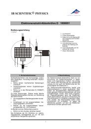
SAMPLE MEASUREMENTS<br />
1. In-phase coupled oscillation<br />
Fig. 3<br />
Angle-time diagram for an in-phase oscillation of coupled pendulums (blue: left-hand pendulum, red: right-hand pendulum). The<br />
angle scale has not been calibrated.<br />
3 / 5
UE105060<br />
<strong>3B</strong> SCIENTIFIC® PHYSICS EXPERIMENT<br />
2. Out-of-phase coupled oscillation<br />
Fig. 4<br />
Angle-time diagram for an out-of-phase oscillation of coupled pendulums (blue: left-hand pendulum, red: right-hand pendulum).<br />
The angle scale has not been calibrated.<br />
3. Oscillation of coupled pendulums with maximum beat amplitude<br />
Fig. 5<br />
Angle-time diagram for an oscillation of coupled pendulums with maximum beat amplitude (blue: left-hand pendulum, red: righthand<br />
pendulum). The angle scale has not been calibrated.<br />
Fig. 6: Magnified view of one beat period in the oscillation of coupled pendulums with maximum beat amplitude (blue: left-hand pendulum,<br />
red: right-hand pendulum). The angle scale has not been calibrated.<br />
4 / 5
UE105060<br />
<strong>3B</strong> SCIENTIFIC® PHYSICS EXPERIMENT<br />
EVALUATION<br />
1. Determine the period of oscillation for coupled pendulums<br />
oscillating in phase<br />
• Open the data entry for the in-phase oscillation.<br />
• Set up the display to include as many complete oscillations<br />
as possible between cursors. The cursors should be<br />
set precisely at points where the oscillation crosses the<br />
axis heading upwards so that a whole number of periods<br />
is included (cf. Fig. 3).<br />
• Read off the time between the cursors from the table<br />
under the display (Fig. 3, red box).<br />
The period of the oscillation is the time between the cursors<br />
divided by the number of complete oscillations included in<br />
that time<br />
27,<br />
8 s<br />
T+<br />
= = 1,<br />
737 s<br />
16<br />
2. Determine the period of oscillation for coupled pendulums<br />
oscillating out of phase<br />
• Open the data entry for the out-of-phase oscillation and<br />
proceed exactly as before.<br />
The period of the oscillation is the time between the cursors<br />
divided by the number of complete oscillations included in<br />
that time<br />
T – = 1,<br />
629 s<br />
3. Determine the period of oscillation for coupled pendulums<br />
oscillating with a maximum beat amplitude<br />
• Open the data entry for the oscillation with the maximum<br />
beat amplitude.<br />
• Set up the cursors so that they include one or more<br />
complete periods of the beat oscillation (cf. Fig. 5) and<br />
read off the time from the table underneath.<br />
The period of the maximum beat amplitude is the time between<br />
the cursors divided by the number of periods of the<br />
beat oscillation included in that time<br />
T∆<br />
= 25<br />
s<br />
• Change the scale of the time axis so that one period of<br />
the beats is displayed in a magnified view.<br />
• Set the cursors so that they include as many oscillations<br />
of one of the pendulums as possible within the space of<br />
one beat (time between successive points where the<br />
pendulums stop still at the rest position - cf. Fig. 6) and<br />
read off the time between the cursors from the table at<br />
the bottom.<br />
The period of the oscillation is the time between the cursors<br />
divided by the number of complete oscillations included in<br />
that time<br />
T = 1,<br />
685 s<br />
4. Compare the measurements for the two periods with<br />
the values as calculated from the intrinsic periods:<br />
For a coupled oscillation with a period T, where the beat<br />
amplitude is at its maximum, the expression below follows<br />
from equation (8):<br />
T+ ⋅T– T = 2 ⋅ = 1,<br />
681 s<br />
(9)<br />
T + T<br />
+<br />
–<br />
Compare this with the measured value of T = 1.685 s.<br />
The beat period T ∆ can also be calculated in a similar way. It<br />
should be noted, however, that this is usually defined to be<br />
the time between successive points where the pendulums<br />
stop still at the rest position. This actually represents only<br />
half the period of the underlying cosine or sine modulation<br />
term in equation (7).<br />
T+<br />
⋅T– T∆ = = 26 s<br />
(10)<br />
T − T<br />
+<br />
–<br />
Compare this answer with the measured value ofT∆ = 25 s .<br />
The difference of about one second between the calculated<br />
and measured values may seem to be quite large at first<br />
glance but it is due to the calculation being highly sensitive<br />
to differences between the intrinsic oscillation periods. If the<br />
intrinsic periods of the two pendulums differ by as little as 4<br />
milliseconds, which roughly corresponds to the maximum<br />
measurement accuracy achievable for the intrinsic oscillation<br />
periods in this experiment, it leads to a difference of a whole<br />
second in the beat period.<br />
5. Determine the spring constant of the spring coupling<br />
the two pendulums<br />
The spring constant D of the spring coupling the pendulums<br />
is related to the coupling constant k as follows:<br />
L<br />
D = k ⋅ ⋅ m<br />
(11)<br />
2<br />
d<br />
(d: distance between the point at which the spring is connected<br />
to the pendulum and the fulcrum of the pendulum)<br />
If the coupling is weak (k