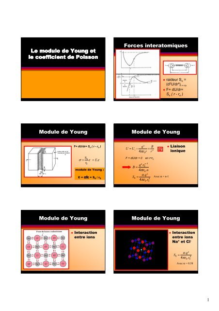
Le module de Young et le coefficient de Poisson Forces ... - Gramme

Le Le module module de de Young Young et et
et
le le coefficient coefficient de de Poisson
Poisson
Module de Young
F= dU/dr= S o ( r - r o )
Module de Young
S0 σ = ε = E.
ε
r
0
module de Young :
E = σ/ε = S 0 / r 0
Interaction
entre ions
Forces interatomiques
raideur S o =
(d 2 U/dr²) r = ro
F= dU/dr=
S o ( r - r o )
Module de Young
q²
B
U = U i − + n
4πε r r
F = dU/dr = 0 en r=r o
0
n−1
q².
r0
B =
4πε 0.
n
α.
q²
S0
=
4πε . r
3
0 0
Avec α = n-1
Liaison
ionique
Module de Young
Interaction
entre ions
Na + et Cl -
S
0
α.
q²
=
4πε . r
3
0 0
Avec α = 0.58
1

Module de Young
Type de liaison S0. en
Nm-1
E en GPa
(approximé par
Covalente, liaison C-C 180
S0/r0
1000 1000 (diamant)
Ionique pure, par ex. Na-CI 9 à 21 30 à 70 250 (Magnésie)
Métallique
Cu-Cu
pure, par ex. 15 à 40 30 à 150 124 (cuivre)
Hydrogène, par ex. H20-H20 2 8 10 (glace)
Van der Waals (cires, 1 2 0.01(caoutchouc)
polymères)
• Caoutchouc :
• température basse : E≈4 Gpa
• température ambiante : E≈0.01 Gpa
Module de Young
Composites
Emesuré en GPa
polymères
• PRFV : les polymères renforcés par fibre de
verre
• PRFC : les polymères renforcés par fibre de
carbone
• PRFB : les polymères renforcés par fibre de
bore
• polymères chargés : des polymères renforcés
par de la poudre de verre ou de silice
• le bois : composite naturel de lignine
(polymère amorphe) rigidifiée par des fibres
de cellulose.
Module de Young
Caoutchouc
• température basse :
• liaisons VDW + ponts covalents
occasionnels
temp tempéééérature temp temp rature rature rature de de de de transition transition transition transition vitreuse, vitreuse, vitreuse, vitreuse, Tg Tg Tg Tg
• température ambiante :
• ponts covalents occasionnels
raideur
Module de Young
Comment le module de Young des
polymères ?
En En ll’associant
l associant
associant à un un mat matériau mat riau plus plus rigide
rigide
Mat Matériaux Mat
Matériaux Mat Mat riaux riaux composites
composites
composites
Composites
Matériau E en GPa
PRFV 7-45
PRFC 70-200
Polyesters 1-5
Bois courants (// aux fibres) 9-16
Bois courants (⊥. aux fibres) 0,6-1,0
2

Module de Young
Calcul du module d’un
composite contenant une
fraction volumique V f de fibres
• // aux fibres
• ⊥ aux fibres
Module de Young
Traction ⊥ aux fibres
E composite =
composite = 1 / / ( ( V f /E
f /Ef +
f + (1- (1-V V f )
f ) /E /Em )
m )
Application 1
Composite : 40% vol fibres de
verre (E=69 GPa), 60% vol résine
(E=3.4 GPa)
• Calculer E composite,long et E composite,transv
30 30GPa GPa
• si section = 250mm² et σ long=50 Mpa,
• calculer F f et F m
• calculer ε f et ε m
5.5 5.5GPa GPa
F f= 11.64
f= 11.64kN, kN, F m= 0.86
m= 0.86kN kN
εf=1.69 10-3 = εm=1.69 10-3 εf=1.69 10-3 = εm=1.69 10-3 Module de Young
Traction // aux fibres
E composite =V
composite =Vf E
f Ef +
f + (1 (1 --V V f )E
f )Em m
Module de Young
Coefficient de Poisson
cristaux
3

Coefficient de Poisson
Caoutchoucs
•ν ≈ 0.5 (pas de variation de volume
lors de la déformation : voir RDM)
Application 2
Tige cylindrique en laiton φ10mm
(E=97 GPa, υ = = 0.34) 0.34) soumise soumise soumise à
traction traction
traction
• Calculer la charge nécessaire pour
rétrécir le diamètre de 2.5 10-3 mm
5600 N
Résistance en traction
Résistance de
cohésion >>>
Limite élasticité
• ex. Acier : limite
élastique 235 MPa
et E=210 000 Mpa
• Pourquoi?
A cause des imperfections !!!
Coefficient de Poisson
Application 3
Quel matériau choisir pour réaliser un
plancher le plus léger possible, pour une
déformabilité (δ/p /p /p) /p et une portée données
L
p
δ
δ=5 pL4 δ=5 pL / (384 EI)
4 / (384 EI)
1m
E (Gpa) Masse vol (g/cm³)
PRFC 220 1.7
Bois 16 0.8
PRFV 45 2.1
Aluminium 69 2.7
Béton 30 2.5
Acier 210 7.8
4