LES ANALYSES CANONIQUES SIMPLE ET GÉNÉRALISÉE ...

More documents

Recommendations

Info

82 v. nzobounsana, s. gaymard démonstration 3. Pour avoir les résultats de la proposition précédente, on dérive l’égalité (30) par rapport aux p vecteurs P (s) 1 , P (s) 2 , · · · , P (s) p . En dérivant (30) par rapport à P (s) 1 , P (s) 2 , · · · , et P (s) p et en égalant à zéro le résultat, on trouve : p j=1,j=i Σ x i x j P (s) j (s) − λiP i − (s−1) Ce qui implique, en multipliant cette dernière équation par t P (k) i p j=1,j=i k=1 En remplaçant β k i dans l’équation (31), on montre que : p j=1,j=i β k i P (k) i = 0 ∀i (31) t P (k) i Σ x i x j P (s) j = β k i ∀i et k (32) [Imi − (s−1) k=1 P k i t P (k) i ]Σ x i x j P (s) j c’est-à-dire que les vecteurs P (s) 1 , P (s) 2 , · · · , P (s) p S (s) (puisque M (s) j 3.4.2. Méthode Ssqcor (s) (s) P j = P j ). (s) = λiP i : (33) vérifient bien le système d’équation Cette généralisation de l’analyse canonique est due à [Kettering, 1971]. Elle consiste à trouver p combinaisons linéaires normées, Z1, Z2, · · · , Zp, appelées variables canoniques qui maximisent la fonction f2(P1, P2, · · · , Pp) = p p i=1 j=i Cor 2 (X i Pi, X j Pj). (34) Les solutions de ce problème d’optimisation sont obtenues de la manière suivante. • Solutions d’ordre un du problème. Au premier pas, il s’agit de trouver p vecteurs canoniques, P1, P2, · · · , Pp, normés (puisque l’on a supposé que dans les groupes, les variables sont deux à deux orthogonales et normées) associés aux p variables canoniques, Z1, Z2, · · · , Zp, qui maximisent la fonction f2(P1, P2, · · · , Pp). Pour ce faire, on utilise la méthode des multiplicateurs de Lagrange. Soient λ1, λ2, · · · , λp p multiplicateurs de Lagrange, cela conduit, pour tout i, à résoudre le système d’équations: ∂L(P1, · · · , Pp) = 0 où L(P1, · · · , Pp) = ∂Pi p Cor 2 (Zi, Zj) − i=1 j=i p λi( t PiPi − 1) (35) Un raisonnement analogue à celui utilisé avec la méthode Sumcor permet de voir que sous la contrainte t PiPi = 1, les vecteurs canoniques qui maximisent la fonction f2(P1, P2, · · · , Pp) vérifient l’équation matricielle : i=1
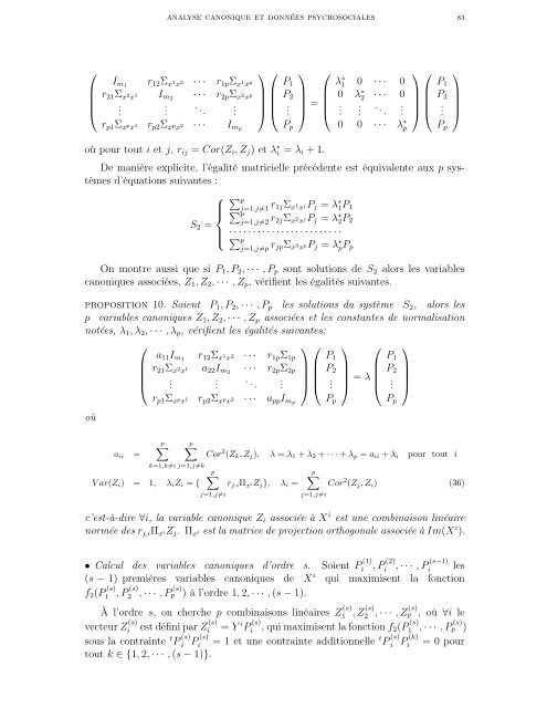
⎛ ⎜ ⎝ analyse canonique et données psychosociales 83 Im1 r12Σx1x2 · · · r1pΣx1xp r21Σx2x1 Im2 · · · r2pΣx2xp . . . .. rp1Σ x p x 1 rp2Σ x p x 2 · · · Imp . ⎞ ⎛ ⎟ ⎜ ⎟ ⎜ ⎟ ⎜ ⎠ ⎝ où pour tout i et j, rij = Cor(Zi, Zj) et λ ∗ i = λi + 1. P1 P2 . Pp ⎞ ⎛ λ∗ 1 0 · · · 0 0 λ∗ 2 · · · 0 ⎞ ⎛ ⎟ ⎠ = ⎜ ⎝ . . . .. . 0 0 · · · λ∗ ⎟ ⎜ ⎟ ⎜ ⎟ ⎜ ⎠ ⎝ p De manière explicite, l’égalité matricielle précédente est équivalente aux p systèmes d’équations suivantes : S2 = ⎧ ⎪⎨ ⎪⎩ p j=1,j=1 r1jΣ x 1 x jPj = λ ∗ 1P1 p j=1,j=2 r2jΣ x 2 x jPj = λ ∗ 2P2 · · · · · · · · · · · · · · · · · · · · · · · · p j=1,j=p rjpΣ x 3 x pPj = λ ∗ pPp On montre aussi que si P1, P2, · · · , Pp sont solutions de S2 alors les variables canoniques associées, Z1, Z2, · · · , Zp, vérifient les égalités suivantes. proposition 10. Soient P1, P2, · · · , Pp les solutions du système S2, alors les p variables canoniques Z1, Z2, · · · , Zp associées et les constantes de normalisation notées, λ1, λ2, · · · , λp, vérifient les égalités suivantes: ⎛ a11Im1 ⎜ r21Σx2x1 ⎜ ⎝ . r12Σx1x2 a22Im2 . · · · · · · . .. ⎞ ⎛ ⎞ ⎛ ⎞ r1pΣ1p P1 P1 r2pΣ2p ⎟ ⎜ ⎟ ⎜ P2 ⎟ ⎜ ⎟ ⎜ P2 ⎟ ⎟ ⎜ ⎟ = λ ⎜ ⎟ . ⎠ ⎝ . ⎠ ⎝ . ⎠ où aii = rp1Σ x p x 1 rp2Σ x p x 2 · · · appImp p p k=1,k=i j=1,j=k V ar(Zi) = 1, λiZi = { Pp Cor 2 (Zk, Zj), λ = λ1 + λ2 + · · · + λp = aii + λi pour tout i p j=1,j=i rj,iΠ x iZj}, λi = p j=1,j=i Pp P1 P2 . Pp ⎞ ⎟ ⎠ Cor 2 (Zj, Zi) (36) c’est-à-dire ∀i, la variable canonique Zi associée à X i est une combinaison linéaire normée des rj,iΠ x iZj. Π x i est la matrice de projection orthogonale associée à Im(X i ). • Calcul des variables canoniques d’ordre s. Soient P (1) i , P (2) i , · · · , P (s−1) (s − 1) premières variables canoniques de X i les i qui maximisent la fonction f2(P (s) 1 , P (s) 2 , · · · , P (s) p ) à l’ordre 1, 2, · · · , (s − 1). À l’ordre s, on cherche p combinaisons linéaires Z (s) 1 , Z (s) 2 , · · · , Z (s) p , où ∀i le vecteur Z (s) i est défini par Z (s) i sous la contrainte t P (s) i P (s) i tout k ∈ {1, 2, · · · , (s − 1)}. = Y i P (s) i , qui maximisent la fonction f2(P (s) 1 , · · · , P (s) p ) = 1 et une contrainte additionnelle t P (s) i (k) P i = 0 pour
Page 1 and 2: Math. & Sci. hum. / Mathematics and
Page 3 and 4: analyse canonique et données psych
Page 11 and 12: ⎛ ⎜ ⎝ Im1 Σx1x2 · · · Σx
Page 13: analyse canonique et données psych
Page 17 and 18: i=1 analyse canonique et données p
Page 33: analyse canonique et données psych

LES ANALYSES CANONIQUES SIMPLE ET GÉNÉRALISÉE ...

You also want an ePaper? Increase the reach of your titles

Delete template?

Save as template?