
You also want an ePaper? Increase the reach of your titles
YUMPU automatically turns print PDFs into web optimized ePapers that Google loves.
<strong>Exercices</strong> <strong>de</strong> <strong>courant</strong> <strong>continu</strong><br />
I.<br />
1) Déterminer e pour que la puissance reçue par la source <strong>de</strong> tension <strong>de</strong> fem e soit<br />
maximum.<br />
2) Quel est alors le ren<strong>de</strong>ment énergétique, défini comme le rapport <strong>de</strong> l’énergie reçue<br />
par la source <strong>de</strong> tension à l’énergie fournie par la source <strong>de</strong> <strong>courant</strong> <br />
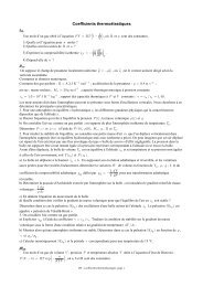
II.<br />
Un générateur <strong>de</strong> fem E = 20 V et <strong>de</strong> résistance interne nulle sert à recharger une<br />
batterie électrochimique <strong>de</strong> fem e et <strong>de</strong> résistance interne r = 1 Ω .<br />
1) Au début, la batterie est déchargée : e = 0 . Quel <strong>courant</strong> i traverse la batterie <br />
Précisez son sens.<br />
2) Lorsque e n'est pas nul, exprimer i en fonction <strong>de</strong> Eeabr ,,,, .<br />
3) Pour quelle valeur <strong>de</strong> e le <strong>courant</strong> i s'annule-t-il <br />
4) Décrire qualitativement l'évolution <strong>de</strong> e et i au cours du temps.<br />
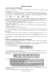
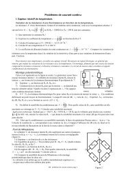
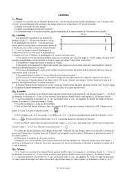
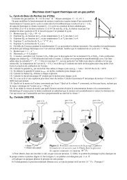
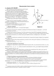
III 53 . Mesure d’une résistance.<br />
On désire mesurer la résistance R à l’ai<strong>de</strong> du montage ci-contre, où le<br />
voltmètre V est équivalent à une résistance R v .<br />
1) Comment faut-il choisir le voltmètre pour minimiser son influence Pour<br />
quelle genre <strong>de</strong> résistance R cela est-il possible <br />
2) Exprimer U en fonction <strong>de</strong>s autres gran<strong>de</strong>urs du schéma dans les <strong>de</strong>ux cas :<br />
a) le <strong>courant</strong> dans le voltmètre est négligeable ;<br />
b) le <strong>courant</strong> dans le voltmètre n’est pas négligeable.<br />
e,r<br />
η<br />
E<br />
R 1<br />
R<br />
b = 3 Ω<br />
a = 3 Ω<br />
3) Désormais, on suppose le <strong>courant</strong> dans le voltmètre négligeable. La sensibilité du montage est s = dU/dR. Justifier<br />
cette définition.<br />
4) Calculer la sensibilité.<br />
5) Comment faut-il choisir R 1 pour maximaliser la sensibilité <br />
IV 41 .<br />
1) Une alimentation <strong>de</strong> résistance R et <strong>de</strong> fem E donnés débite dans un dipôle D. Pour quelle<br />
tension u à ses bornes le dipôle D reçoit-il la puissance maximum <br />
2) D a une caractéristique rectiligne ; sa résistance est r et sa fem, qui s’oppose au passage du<br />
<strong>courant</strong>, est e . A quelle(s) condition(s) sur e, r la puissance reçue par D est-elle maximale <br />
3) A quelle(s) condition(s) sur e, r la puissance reçue par la fem e est-elle maximale <br />
V 30 .<br />
1) Pour mesurer la fem E d’un générateur à caractéristique rectiligne, on réalise une boucle avec ce générateur, un<br />
autre générateur à caractéristique rectiligne <strong>de</strong> fem connue E 2 V inférieure à E , une résistance et un ampèremètre<br />
qui mesure, selon le sens <strong>de</strong> branchement du générateur <strong>de</strong> fem inconnue, un <strong>courant</strong> i 1 = 3mA<br />
ou i 2 = 1mA , toujours<br />
dans le même sens et en utilisant le même calibre. Calculer E .<br />
2) On admet que les erreurs commises par l’ampèremètre lors <strong>de</strong>s <strong>de</strong>ux mesures sont indépendantes, que l’incertitu<strong>de</strong><br />
sur chaque mesure est ∆i = 0,005mA et que l’incertitu<strong>de</strong> sur E0<br />
est ∆E 0 = 1mV<br />
. Quelle est l’incertitu<strong>de</strong> sur E <br />
VI 54 .<br />
R = 1MΩ . Quand l’interrupteur est fermé, le voltmètre V, qui équivaut à une résistance<br />
RV<br />
, indique U 1 = 11V ; quand il est ouvert, V indique U 2 = 10 V . Calculer RV<br />
.<br />
0 =<br />
E<br />
R<br />
E<br />
R<br />
R<br />
V<br />
e,r<br />
V<br />
e<br />
U<br />
D<br />
VII 80 .<br />
Exprimer le <strong>courant</strong> i en fonction <strong>de</strong> abRE ,, , , E .<br />
1 2<br />
a<br />
b<br />
i<br />
R<br />
b<br />
a<br />
E 1<br />
E 2<br />
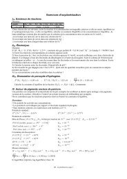
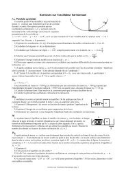
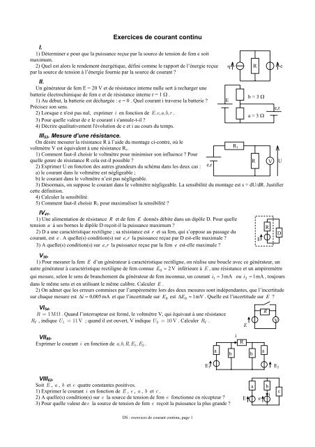
VIII 62 .<br />
Soit E , a , b et c quatre constantes positives.<br />
1) Exprimer le <strong>courant</strong> i en fonction <strong>de</strong> E , e , a , b et c .<br />
2) A quelle(s) condition(s) sur e la source <strong>de</strong> tension <strong>de</strong> fem e fonctionne en récepteur <br />
3) Pour quelle valeur <strong>de</strong>e la source <strong>de</strong> tension <strong>de</strong> fem e reçoit la puissance la plus gran<strong>de</strong> <br />
E<br />
a<br />
e<br />
b<br />
i<br />
c<br />
DS : exercices <strong>de</strong> <strong>courant</strong> <strong>continu</strong>, page 1
IX 21 . Ligne <strong>de</strong> quadripôles en Π.<br />
1) Exprimer R2<br />
en fonction <strong>de</strong> R1<br />
et R pour que le groupement <strong>de</strong> la première<br />
figure ait entre A et B la résistance R . Dans la suite, R2<br />
possè<strong>de</strong> cette valeur. A<br />
quelle condition cela est-il possible <br />
2) Exprimer alors le rapport <strong>de</strong>s tensions à la sortie et à l’entrée H = vs<br />
/ ve<br />
.<br />
3) Montrer que la résistance entre C et D du groupement <strong>de</strong> la secon<strong>de</strong><br />
figure est égale à R .<br />
C<br />
4) Exprimer en fonction <strong>de</strong> R 1 et R le rapport <strong>de</strong>s tensions à la sortie v e<br />
et à l’entrée H′ = v′<br />
/ v .<br />
D<br />
s<br />
5) Que vaut H′′ = vs′′<br />
/ ve<br />
pour la troisième<br />
figure <br />
e<br />
v e<br />
R 2<br />
R 2<br />
R1<br />
R1 /2<br />
R 1<br />
ve<br />
R 2<br />
R 2<br />
R 1 /2<br />
A<br />
B<br />
R 2<br />
R<br />
R 1<br />
1<br />
R 2<br />
R1 /2<br />
R 2<br />
R 1 /2<br />
R 1<br />
R 1<br />
R<br />
R<br />
R<br />
v s<br />
v′<br />
s<br />
v′′<br />
s<br />
X 43 .<br />
Exprimer i en fonction <strong>de</strong> a, b, c, d ,E et I dans la figure ci-contre.<br />
E<br />
i<br />
a<br />
b<br />
c<br />
I<br />
d<br />
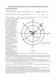
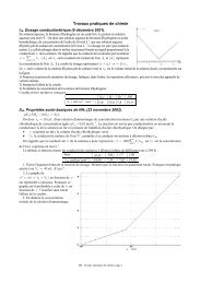
XI 41 . d’après ENAC pilotes 1999.<br />
1) A l'ai<strong>de</strong> d'un fil métallique homogène <strong>de</strong> section constante, on réalise un circuit<br />
constitué <strong>de</strong> <strong>de</strong>ux conducteurs (figure 4) :<br />
– l'un a la forme d'un cercle <strong>de</strong> centre O ;<br />
– l'autre est un diamètre AB du cercle.<br />
Le conducteur diamétral possè<strong>de</strong> une résistance 2 r . Dans toute la suite, on conservera<br />
le nombre π dans les expressions <strong>de</strong>s différents <strong>courant</strong>s et résistances à calculer.<br />
Calculer la résistance r ′ d’un <strong>de</strong>mi cercle.<br />
2) On ajoute sur l’un <strong>de</strong>s <strong>de</strong>micercles AB, comme<br />
l'indique la figure 5, une source <strong>de</strong> tension <strong>continu</strong>e <strong>de</strong> f.é.m. E. Calculer l'intensité I AB<br />
du <strong>courant</strong> qui circule dans le conducteur diamétral<br />
AB.<br />
3) On considère le circuit <strong>de</strong> la figure 6 obtenu en<br />
ajoutant à celui <strong>de</strong> la figure 4 :<br />
– un autre conducteur diamétral CD perpendiculaire à<br />
AB et relié à lui en 0, fait du même fil métallique ;<br />
– <strong>de</strong>ux sources <strong>de</strong> tension <strong>continu</strong>e <strong>de</strong> f.é.m. E (figure<br />
6). Quelles sont les opérations <strong>de</strong> symétrie ou d’antisymétrie qui laissent invariant ce<br />
montage Calculer les intensités I AD = I et I DB qui circulent respectivement dans les<br />
arcs AD et DB.<br />
4) On ajoute cette fois ci quatre sources <strong>de</strong> tension i<strong>de</strong>ntiques et non plus <strong>de</strong>ux<br />
(figure 7). Quelles sont les opérations <strong>de</strong> symétrie ou d’antisymétrie qui laissent<br />
invariant ce montage Calculer les intensités <strong>de</strong>s <strong>courant</strong>s I AD et I D0 .<br />
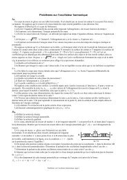
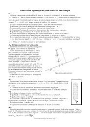
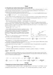
XII 57 . Recherche d’un défaut d’isolement.<br />
1) MONTAGE DIVISEUR <strong>de</strong> TENSION.<br />
Une pile <strong>de</strong> fem e et <strong>de</strong> résistance r alimente <strong>de</strong>ux résistances R1<br />
et R2<br />
disposées en série.<br />
a) Exprimer la tension u = V(A) – V(B) aux bornes <strong>de</strong> R 2 en fonction <strong>de</strong> e, r, R 1 et R 2 .<br />
b) Que <strong>de</strong>vient u si R 1 est infini et R 2 fini <br />
c) Que <strong>de</strong>vient u si R 1 est fini et R 2 infini <br />
2) RECHERCHE d'un DEFAUT d'ISOLEMENT.<br />
Un appareil comporte trois réseaux formés <strong>de</strong> fils <strong>de</strong> très faibles résistances, qu'on peut<br />
R 1<br />
A<br />
R 2<br />
e,r<br />
B<br />
schématiser par trois points A, B et C. Si l'appareil est en bon état, ces trois points sont isolés. Mais il peur y avoir aussi<br />
un défaut d'isolement, que l'on peut schématiser par une résistance finie située entre <strong>de</strong>ux <strong>de</strong> ces points :<br />
DS : exercices <strong>de</strong> <strong>courant</strong> <strong>continu</strong>, page 2
A<br />
A<br />
A<br />
A<br />
B<br />
C<br />
appareil en bon état<br />
B<br />
défaut 1<br />
C<br />
B<br />
défaut 2<br />
C<br />
B<br />
défaut 3<br />
C<br />
Pour rechercher s'il existe un ou plusieurs <strong>de</strong> ces défauts d'isolement, on branche entre <strong>de</strong>ux <strong>de</strong>s points A, B et C un<br />
générateur <strong>de</strong> force électromotrice e = 2,2 volts et <strong>de</strong> résistance interne r = 0,1 ohm et un voltmètre <strong>de</strong> résistance R V =<br />
30 000 ohms et on lit la tension u affichée par le voltmètre :<br />
a) si le générateur est branché entre A et B, tandis que le voltmètre l’est entre B et C, alors u = 0,2 volt ; que peut-on<br />
en déduire sur la position <strong>de</strong>s défauts d'isolement possibles <br />
b) si le générateur est branché entre A et B, tandis que le voltmètre l'est entre A et C, alors u = 0 ; que peut-on en<br />
déduire sur la position <strong>de</strong>s défauts d'isolement possibles <br />
c) si le générateur est branché entre B et C, tandis que le voltmètre l'est entre A et C, alors u = 0 ; que peut-on en<br />
déduire sur la position <strong>de</strong>s défauts d'isolement possibles <br />
d) En déduire où se trouve le (ou les) défaut d'isolement et sa (ou ses) valeur.<br />
Réponses<br />
I. 1) e = Rη<br />
/2 ; 2) 0,5.<br />
aE<br />
aE − ( a + b)<br />
e aE<br />
II. 1) i =<br />
= 4A mesuré en sens contraire <strong>de</strong> e ; 2) i =<br />
; 3) e<br />
10 V<br />
ab + ( a + b)<br />
r<br />
ra ( + b)<br />
+ ab<br />
= a + b<br />
= .<br />
III. 1) R >> R possible si R n’est pas trop grand ; 2) U<br />
V<br />
Re<br />
= ou U<br />
r + R + R<br />
r + R1<br />
4) s =<br />
2<br />
e ; 5) si R < r , l’optimum est R = 0 , sinon R .<br />
( r + R +<br />
1 1 = R − r<br />
R)<br />
1<br />
IV. 1) u = E/2 ; 2) 2 Re + rE = RE ; 3) r = 0, e = E/2.<br />
i1 + i2<br />
∆E ∆E0 2∆i1 −3<br />
V. 1) E = E0 = 4V ; 2) = + = 5,5.10 ∆ E = 22 mV .<br />
i1 − i2<br />
E E0 i1 − i2<br />
R<br />
VI. RV<br />
= 10 M<br />
U / U − 1<br />
= Ω .<br />
1 2<br />
( 1 − E2)<br />
( )<br />
b E<br />
VII. i =<br />
2ab + R a + b<br />
.<br />
cE − ( a + c ) e cE<br />
VIII. 1) i =<br />
; 2) e<br />
( a + b)<br />
c + ab<br />
< a + c<br />
; 3) e =<br />
cE<br />
a + c<br />
.<br />
2( )<br />
1<br />
e<br />
=<br />
;<br />
⎛ 1 1 ⎞<br />
1 + ( + ) ⎜ + ⎠<br />
⎟<br />
r R1<br />
⎜⎝<br />
R R V<br />
2<br />
2<br />
2RR 1<br />
R1<br />
− R vs<br />
IX. 1) R2 = ; R ; 2)<br />
2 2 1 > R H = ; 4)<br />
′ ⎛ R1<br />
− R ⎞ 4<br />
v s 1<br />
= R1<br />
− R<br />
R1<br />
+ R v ⎜<br />
e<br />
⎜⎝R 1 + R⎠⎟<br />
; 5)<br />
′′ R R<br />
=<br />
v ⎜<br />
⎛ − ⎞ e<br />
⎜⎝<br />
R1<br />
+ R⎠⎟<br />
.<br />
E + cI E − dI<br />
X. i = +<br />
a + c b + d<br />
.<br />
E<br />
XI. 1) r′ = πr ; 2) IAB<br />
= ; 3) la bissectrice <strong>de</strong> COA est un axe <strong>de</strong> symétrie, celle <strong>de</strong> DOA est un axe<br />
( 4 + π)<br />
r<br />
2E<br />
d’antisymétrie et O est un centre d’antisymétrie ; I DB = 0 ; IAD<br />
= ; 4) la droite CD est une axe <strong>de</strong><br />
( π + 4 ) r<br />
symétrie, la droite AB est un axe d’antisymétrie et O est une centre<br />
2E<br />
4E<br />
d’antisymétrie ; IAD<br />
= IDO<br />
= .<br />
( π + 4) r ( π + 4)<br />
r<br />
Re 2<br />
XII. 1.a) u = R2i<br />
= ; 1.b) u = 0 ; 1.c) u = e ; 2.a) Il y a une résistance finie entre A et C ; 2.b) Les<br />
r + R1 + R2<br />
bornes B et C sont isolées ; 2.c) Les bornes A et B sont isolées ; 2.d) défaut du type 1 : R = 300000 Ω .<br />
DS : exercices <strong>de</strong> <strong>courant</strong> <strong>continu</strong>, page 3
Corrigé<br />
I.<br />
1) Loi <strong>de</strong>s nœuds : η = i + j<br />
Loi <strong>de</strong>s mailles e = R j<br />
D’où :<br />
e<br />
i = η − P = ei = eη<br />
−<br />
R<br />
dP 2e Rη<br />
= η − > 0 si e <<br />
<strong>de</strong> R<br />
2<br />
2<br />
e<br />
R<br />
Rη<br />
P est maximum quand e =<br />
2<br />
e<br />
ei<br />
η −<br />
2) Le ren<strong>de</strong>ment est =<br />
R<br />
. Il vaut 1/ 2 quand P est maximum.<br />
eη<br />
η<br />
η<br />
R<br />
j<br />
i<br />
e<br />
II.<br />
1)<br />
• Résolution en prenant pour inconnues les <strong>courant</strong>s<br />
ri<br />
Maille <strong>de</strong> droite : ri − aj = 0 ⇒ j =<br />
a<br />
r<br />
Maille <strong>de</strong> gauche : bi ( + j) + aj= E ⇒ ib [ + ( a+ b) ] = E<br />
a<br />
aE<br />
i = = 4A<br />
ab + ( a + b)<br />
r<br />
• Résolution en prenant pour inconnues les potentiels<br />
Le potentiel étant en bas 0 et en haut E , appliquons le théorème <strong>de</strong> Millman au point C :<br />
E<br />
VC<br />
E<br />
VC<br />
= b ⇒ i = =<br />
1 1 1 r<br />
br<br />
+ + b + r +<br />
a b r a<br />
2) Prenons comme inconnues les <strong>courant</strong>s, avec la même notation qu’à la question précé<strong>de</strong>nte.<br />
Maille <strong>de</strong> droite : ri − aj = −e<br />
Maille <strong>de</strong> gauche : b( i + j) + aj = E ⇒ bi + ( a + b)<br />
j = E<br />
Multiplions la première équation par a + b , la secon<strong>de</strong> par a et ajoutons membre à membre :<br />
aE − ( a + b)<br />
e<br />
[( ra+ b) + abi ] = − ( a+ be ) + aE⇒ i=<br />
ra ( + b)<br />
+ ab<br />
On vérifie cette formule en observant qu’elle redonne celle <strong>de</strong> la question précé<strong>de</strong>nte si e = 0 .<br />
aE<br />
3) i = 0 si e = 10 V<br />
a + b<br />
=<br />
4) Au début <strong>de</strong> la charge, e = 0 et i = 4A.<br />
Au cours <strong>de</strong> la charge, e augmente et i diminue.<br />
A la fin, l’évolution s’arrête alors que e = 10 V et i = 0 .<br />
L’énoncé ne permet pas <strong>de</strong> déterminer la durée, finie ou infinie, <strong>de</strong> la charge.<br />
E<br />
C<br />
i + j<br />
b<br />
a<br />
j<br />
r<br />
i<br />
Autre calcul du <strong>courant</strong> <strong>de</strong> charge<br />
Le circuit équivaut aux circuits suivants :<br />
i<br />
i<br />
E<br />
b<br />
b a<br />
r<br />
e<br />
E<br />
b<br />
a<br />
b<br />
r<br />
e<br />
a<br />
b<br />
( a b)<br />
E<br />
b<br />
r<br />
e<br />
DS : exercices <strong>de</strong> <strong>courant</strong> <strong>continu</strong>, page 4
( a b)<br />
E aE<br />
− e − e<br />
( )<br />
D’où b a b aE − a + b e<br />
i = =<br />
+<br />
=<br />
r + ( a b) ab ( a + b)<br />
r + ab<br />
r +<br />
a + b<br />
R 1<br />
III. Mesure d’une résistance.<br />
1. Pour minimiser l’influence du voltmètre, il faut qu’il ait une résistance beaucoup plus gran<strong>de</strong> que R. Cela n’est<br />
possible que si R n’est pas trop grand.<br />
2. Le théorème <strong>de</strong> Millman donne :<br />
e<br />
V = e<br />
V = U<br />
r + R1<br />
e Re<br />
U = = =<br />
1 1 r + R1 r + R + R<br />
+ 1 +<br />
1<br />
r + R R e,r<br />
1<br />
R<br />
e<br />
V = 0<br />
R V<br />
r + R1<br />
e<br />
U = =<br />
.<br />
1 1 1 ⎛ 1 1 ⎞ + +<br />
r R R R<br />
1 ( r R )<br />
+<br />
+ +<br />
1 ⎜ + 1<br />
V<br />
⎜⎝R R ⎠<br />
⎟<br />
3. Le montage est sensible si dU est grand pour dR petit.<br />
u ′ u′ v − uv′<br />
4. En utilisant ( ) =<br />
2<br />
v v<br />
dU<br />
1 1<br />
s = = r + R + R − R r R<br />
2<br />
e =<br />
+<br />
2e .<br />
dR ( r + R + R) ( r + R + R)<br />
1 1<br />
V<br />
U<br />
2<br />
u ′ u ′ v −u2vv ′ u ′ v −2uv<br />
2<br />
= ′<br />
4<br />
=<br />
3<br />
v v v<br />
ds ( r + R + R) − 2( r + R ) R − ( r + R<br />
1 1<br />
= e =<br />
) 1<br />
e<br />
dR ( r + R + R) ( r + R + R)<br />
5. En utilisant ( )<br />
ds<br />
dR<br />
3 3<br />
1 1 1<br />
1<br />
> 0 ⇔ R < R − r<br />
1<br />
Si R < r , l’optimum est R = 0 (la fonction est décroissante sur tout son intervalle <strong>de</strong> définition) ;<br />
1<br />
si R r , l’optimum est R = R − r .<br />
><br />
1<br />
On peut aussi faire le même calcul en utilisant la dérivée logarithmique :<br />
d lns<br />
1 2 R −r −R1<br />
= − =<br />
2<br />
> 0 si R < R − r<br />
1<br />
dR r + R r + R + R ( r + R + R )<br />
1 1 1 1<br />
IV.<br />
E − u<br />
1) La puissance reçue par D est P = u i = u qui est maximum pour u = E /2. Cela se montre <strong>de</strong> plusieurs<br />
R<br />
façons :<br />
• Le maximum du produit <strong>de</strong> <strong>de</strong>ux nombres u et E − u <strong>de</strong> somme E déterminée a lieu quand ces nombres sont<br />
égaux.<br />
•<br />
dP E − 2<br />
= u dP > 0 si u <<br />
E .<br />
du R du<br />
2<br />
• Le graphe <strong>de</strong> Pu ( ) a la forme d’une parabole ; comme P(0) = P ( E) = 0 , Pu ( ) est maximum en u = E /2.<br />
E −e E − e Re + rE E<br />
2) i = u = e + ri = e + r = =<br />
R + r R + r R + r 2<br />
2<br />
. Donc la condition est 2Re + rE = RE . Alors<br />
E<br />
P = , qui ne dépend pas <strong>de</strong> e,<br />
r.<br />
4R<br />
eE ( − e)<br />
eE ( − e)<br />
3) P = ei = qui est une fonction décroissante <strong>de</strong> r , donc maximum pour r = 0 . Alors P =<br />
R + r<br />
R<br />
est maximum pour e = E /2. Donc la condition est r = 0, e = E/2.<br />
V.<br />
1) Soit R le total <strong>de</strong> la résistance extérieure, <strong>de</strong>s résistances <strong>de</strong>s <strong>de</strong>ux générateurs et <strong>de</strong> la résistance <strong>de</strong><br />
l’ampèremètre (qui est la même dans les <strong>de</strong>ux montages, puisque l’ampèremètre est sur le même calibre).<br />
DS : exercices <strong>de</strong> <strong>courant</strong> <strong>continu</strong>, page 5
⎧⎪ E + E0 = Ri1<br />
⎪<br />
⎨<br />
⎪E − E0 = Ri<br />
⎪⎩<br />
2<br />
soit en prenant le rapport membre à membre :<br />
E + E0 i1 i1 i2<br />
= ⇒ E = E<br />
+<br />
0 = 4V<br />
E −E0 i2 i1 −i2<br />
2) Différentions :<br />
ln E = ln E + ln( i + i ) − ln( i −i<br />
)<br />
0 1 2 1 2<br />
dE dE0 d ( i1 + i2) d ( i1 −i2)<br />
dE0<br />
⎡ 1 1 ⎤ ⎡ 1 1 ⎤<br />
= + − = + di1 − + di2<br />
+<br />
E E0 i1 + i2 i1 − i2 E0 ⎢⎣ i1 + i2 i1 − i2 ⎥⎦ ⎢⎣i1 + i2 i1 − i<br />
2 ⎥⎦<br />
En tenant compte <strong>de</strong> ce que les erreurs sur i 1 et i 2 peuvent être <strong>de</strong> sens contraires :<br />
−3<br />
∆E ∆E 1 1 ⎡ 1 1 ⎤ ∆E 2∆ i 10 2 × 0, 005<br />
= + ∆i1 − + ∆ i2<br />
+ = + = + = 5, 5.10<br />
E E0 i1 + i2 i1 − i2 ⎢⎣i1 + i2 i1 −i2 ⎥⎦<br />
E0 i1 −i2<br />
2 3−1<br />
−3<br />
∆ E = 4× 5,5.10 V = 22mV<br />
0 0 1 −3<br />
VI.<br />
Quand l’interrupteur est fermé, E = U 1 .<br />
Quand l’interrupteur est ouvert, le même <strong>courant</strong> i traverse R et V (montage diviseur <strong>de</strong> tension) :<br />
E U2<br />
R<br />
i = = ⇒ R V = = 10 MΩ<br />
R + R R U / U − 1<br />
VII.<br />
V<br />
V<br />
1 2<br />
Résolution en prenant comme inconnues les <strong>courant</strong>s.<br />
Notons les <strong>courant</strong>s comme l’indique la figure. La loi <strong>de</strong> nœuds est<br />
satisfaite. La loi <strong>de</strong> mailles s’écrit :<br />
E1<br />
+ bi<br />
aj + b ( j − i ) = E1<br />
⇒ j =<br />
a + b<br />
E2<br />
− bi<br />
ak + b ( k + i ) = E2<br />
⇒ k =<br />
a + b<br />
Ri + b ( k + i ) −b ( j − i ) = 0<br />
⎡E2 − bi E1<br />
+ bi⎤<br />
( R + 2b)<br />
i + b⎢<br />
− ⎥ = 0<br />
⎣ a + b a + b ⎦<br />
b( E1 −E2 ) b( E1 −E2<br />
)<br />
i = =<br />
2<br />
( R + 2b)( a + b)<br />
− 2b<br />
2ab + R( a + b )<br />
Résolution en prenant comme inconnues les potentiels.<br />
Notons les potentiels comme l’indique la figure et appliquons le<br />
théorème <strong>de</strong> Millman aux <strong>de</strong>ux bornes <strong>de</strong> R :<br />
E1 v E2<br />
u<br />
+ +<br />
u =<br />
a R<br />
v =<br />
a R<br />
1 1 1 1 1 1<br />
+ + + +<br />
a b R a b R<br />
E1 −E2<br />
v −u<br />
+<br />
u − v =<br />
a R<br />
1 1 1<br />
+ +<br />
a b R<br />
E1 − E2<br />
a bR( E1 − E2<br />
)<br />
u − v = =<br />
1 1 2 2ab + R( a + b )<br />
+ +<br />
a b R<br />
u −v b( E1 −E2<br />
)<br />
i = =<br />
R 2ab + R( a + b)<br />
j<br />
i<br />
R<br />
a<br />
b b<br />
a<br />
j – i<br />
E 1 k + i E 2<br />
V = u V = v<br />
R<br />
a<br />
a<br />
b b<br />
V = E 1<br />
V = E 2<br />
E 1<br />
V = 0<br />
k<br />
E 2<br />
DS : exercices <strong>de</strong> <strong>courant</strong> <strong>continu</strong>, page 6
Résolution par équivalences entre modèle <strong>de</strong><br />
Thévenin et modèle <strong>de</strong> Norton.<br />
Remplaçons les groupements { E1,<br />
a}<br />
et { E2,<br />
a}<br />
par<br />
leurs modèles <strong>de</strong> Norton, groupons les résistances en<br />
parallèle et enfin remplaçons les <strong>de</strong>ux groupements<br />
formés d’une source <strong>de</strong> <strong>courant</strong> et d’une résistance en<br />
parallèle par leurs modèles <strong>de</strong> Thévenin ; ceci montre<br />
l’équivalence <strong>de</strong>s quatre montages <strong>de</strong>ssinés à droite. Le<br />
<strong>de</strong>rnier montre que<br />
b( E1 − E2<br />
)<br />
a + b b( E1 − E2<br />
)<br />
i = =<br />
.<br />
2ab R( a + b)<br />
+ 2ab<br />
R + a + b<br />
E 1 /a<br />
E 1<br />
E 1 /a<br />
i<br />
R<br />
a<br />
a<br />
b b<br />
i<br />
R<br />
a b b a<br />
i<br />
R<br />
ab/(a+b) ab/(a+b)<br />
E 2<br />
E 2 /a<br />
E 2 /a<br />
bE 1 /(a+b)<br />
i<br />
R<br />
ab/(a+b) ab/(a+b)<br />
bE 2 /(a+b)<br />
VIII.<br />
1) Cette question peut être résolue :<br />
• en prenant comme inconnue u le potentiel du nœud d’en haut et en appliquant le<br />
V = u<br />
E e<br />
+<br />
c( bE ae)<br />
théorème <strong>de</strong> Millman : a b<br />
+<br />
u = =<br />
, d’où<br />
a b<br />
1 1 1 ab + bc + ca<br />
c<br />
+ +<br />
V = E i V = e<br />
a b c<br />
E e<br />
u − e c( bE + ae)<br />
cE − ( a + c)<br />
e<br />
i = = ( − e)<br />
/ b =<br />
;<br />
V = 0<br />
b ab + bc + ca ab + bc + ca<br />
• en remplaçant la branche <strong>de</strong> gauche par son modèle <strong>de</strong> Norton, en groupant sa résistance avec la branche <strong>de</strong> droite<br />
et en revenant au modèle <strong>de</strong> Thévenin :<br />
E<br />
a<br />
a<br />
b<br />
e i<br />
c<br />
E<br />
a<br />
b<br />
ac<br />
a + c e i<br />
cE<br />
a + c<br />
ac<br />
a + c<br />
e<br />
b<br />
i<br />
cE ac cE − ( a + c ) e<br />
= − + =<br />
.<br />
a + c a + c ab + bc + ca<br />
• ou en prenant comme inconnues les <strong>courant</strong>s, comme ci-contre et en appliquant la loi <strong>de</strong>s mailles :<br />
E − e = a ( i + j ) + bi e = − bi + cj<br />
i+j<br />
e + bi a( e + bi) cE − ( a + c)<br />
e<br />
d’où j = E − e = ( a + b)<br />
i + i =<br />
c<br />
c<br />
( a + b)<br />
c + ab .<br />
d’où i ( e) /( b)<br />
cE<br />
2) P = e i > 0 ⇒ 0 < e < .<br />
a + c<br />
2<br />
( )<br />
3)<br />
cEe − a + c e dP cE − 2( a + )<br />
P = e i = ⇒ = c e dP > 0 ⇒ e <<br />
cE donc P est maximum<br />
( a + b)<br />
c + ab <strong>de</strong> ( a + b) c + ab <strong>de</strong> 2( a + c)<br />
pour e =<br />
cE<br />
a + c<br />
2( )<br />
.<br />
j<br />
DS : exercices <strong>de</strong> <strong>courant</strong> <strong>continu</strong>, page 7
R<br />
IX.<br />
1 1 1 1 1 1 R1<br />
− R<br />
1) R1 ( R 2 + ( R1<br />
R)<br />
) = R ⇒ + = = − =<br />
R1 RR 1 R RR 1 R R1<br />
RR<br />
R<br />
1<br />
2 + R2<br />
+<br />
R + R R + R<br />
2<br />
RR 1 RR 1 2RR<br />
1<br />
2 + = R2 =<br />
R<br />
2 2<br />
1 + R R1 − R R1<br />
− R<br />
.<br />
1 1<br />
Comme une résistance est positive, ce n’est possible que si R1<br />
2) Le même <strong>courant</strong> i traverse successivement R et R R :<br />
2<br />
1 <br />
> R .<br />
ve<br />
vs<br />
1 1 1 1<br />
i = − = v ⎛ s ve vs<br />
1 R2<br />
R ⎞ ⎛ ⎛<br />
⎜<br />
+ ⇒ = + +<br />
2 ⎝ R1 R⎠⎟<br />
⎝ ⎜ ⎝ ⎜R<br />
⎟<br />
1 R⎞⎞⎟ ⎠⎠<br />
ve<br />
R2<br />
vs<br />
1<br />
Cette relation s’obtient aussi par le théorème <strong>de</strong> Millman : v s = ⇒ =<br />
1 1 1 ve<br />
⎛ 1 1 ⎞ + + 1 + R2<br />
R R R ⎜ +<br />
⎜⎝R R ⎠<br />
⎟<br />
1 1 1 R1<br />
− R<br />
H = = = =<br />
⎛ ⎞ 2R R<br />
1<br />
1 + R<br />
1 + R<br />
⎞<br />
⎜<br />
+ 1<br />
+<br />
⎝ ⎠ ⎜⎝ ⎠<br />
⎟ R − R<br />
1 1 2<br />
2RR<br />
1 ⎛ 1 1<br />
2 ⎜<br />
R 2 2<br />
1 R ⎟ + +<br />
R1<br />
− R ⎜ R1<br />
R<br />
1<br />
2 1 1<br />
3) La résistance R équivaut à <strong>de</strong>ux résistances R disposées en parallèle. le montage est constitué <strong>de</strong> l’ensemble<br />
1 /2 1<br />
<strong>de</strong> la résistance R et du quadripôle en Π <strong>de</strong> la question 1, équivalent à une résistance R , le tout précédé d’un autre<br />
quadripôle en Π, qui est équivalent avec ce qui le suit à une résistance R .<br />
vs<br />
R1<br />
− R<br />
4) Si v s est la tension entre les <strong>de</strong>ux quadripôles en Π, d’après la question 2, =<br />
v R + R<br />
, vs′ R1<br />
− R<br />
=<br />
v R + R<br />
, d’où<br />
2<br />
s<br />
′ ⎛ 1 − ⎞ ⎟<br />
v R R<br />
= v ⎜⎝<br />
R + R⎠⎟<br />
e<br />
1<br />
.<br />
5) A présent, on a interposé quatre quadripôles en Π ; chacun, placé <strong>de</strong>vant une résistance R , donne à l’ensemble la<br />
même résistance R et multiplie la tension par H ; d’où :<br />
4<br />
s<br />
′′ ⎛ 1 − ⎞ ⎟<br />
v R R<br />
= v ⎜⎝<br />
R + R⎠⎟<br />
e<br />
1<br />
.<br />
e<br />
1<br />
s<br />
1<br />
X.<br />
Loi <strong>de</strong>s mailles pour ( Eac , , ) et ( Ebd ,, ) :<br />
E + cI<br />
E = aj + c( j −I ) ⇒ j =<br />
a + c<br />
E − dI<br />
E = bk + d( k + I ) ⇒ k =<br />
b + d<br />
E + cI E − dI<br />
Loi <strong>de</strong>s nœuds : j + k = i = +<br />
a + c b + d<br />
.<br />
E<br />
i<br />
a<br />
j – I<br />
c<br />
j<br />
I<br />
k<br />
b<br />
I + k<br />
d<br />
XI.<br />
1) Si R est le rayon, les longueurs du diamètre et du <strong>de</strong>mi cercle sont 2 R et πr<br />
. Comme la résistance est<br />
r′ πR<br />
proportionnelle à la longueur, = ⇒ r′<br />
= π r .<br />
2r<br />
2R<br />
2) Une carte <strong>de</strong>s potentiels pour un montage équivalent est représentée ci-contre : l’origine <strong>de</strong>s <strong>de</strong>ux<br />
flèches est au potentiel nul, tandis que leurs extrémités sont aux potentiels E et u . Le théorème <strong>de</strong><br />
E<br />
πr<br />
u E<br />
Millman donne u = V ( A) − V ( B)<br />
=<br />
πr<br />
⇒ IAB<br />
= = .<br />
1 1 1<br />
2r<br />
( 4 + π)<br />
r<br />
2r<br />
+ +<br />
πr πr 2r<br />
πr<br />
3) La bissectrice <strong>de</strong> COA est un axe <strong>de</strong> symétrie. Celle <strong>de</strong> DOA est un axe d’antisymétrie. O est un<br />
centre d’antisymétrie.<br />
u<br />
La première symétrie montre que V ( B ) = V ( D) , donc que I DB = 0 , et <strong>de</strong> même I AC = 0 .<br />
π<br />
2E<br />
La loi <strong>de</strong>s mailles appliquée à la maille ADOA donne : E = ( + 2<br />
2<br />
) r I ⇒ IAD<br />
= .<br />
( π + 4)<br />
r<br />
E<br />
DS : exercices <strong>de</strong> <strong>courant</strong> <strong>continu</strong>, page 8
4) La droite CD est une axe <strong>de</strong> symétrie, la droite AB est un axe d’antisymétrie et O est une centre<br />
d’antisymétrie.<br />
Les points A, O et B, situés sur un axe d’antisymétrie sont à un potentiel nul, donc la branche AB<br />
est parcourue par un <strong>courant</strong> nul et peut être supprimée sans perturber le montage. La carte <strong>de</strong>s<br />
<strong>courant</strong>s est celle ci-contre.<br />
La loi <strong>de</strong>s mailles appliquée à la maille ADOCA donne :<br />
2E<br />
4E<br />
2E = π ri + 2 r.2i ⇒ IAD<br />
= IDO<br />
= .<br />
( π + 4) r ( π + 4)<br />
r<br />
XII.<br />
A<br />
Re 2<br />
1.a) e = ( r + R1 + R2 ) i u = R2i<br />
=<br />
r + R1 + R2<br />
2, 2 V R<br />
1.b) u = 0<br />
0, 2 V<br />
1.c) u = e<br />
2.a) Il y a donc une résistance finie entre A et C.<br />
B<br />
C<br />
2.b) Les bornes B et C sont isolées.<br />
R V = 30000 Ω<br />
2.c) Les bornes A et B sont isolées.<br />
2.d) On déduit <strong>de</strong>s trois essais qu’il y a un défaut du type 1 : il y a un défaut d’isolement, qui se traduit par la<br />
résistance R . Le montage lors <strong>de</strong> l’essai a) est un diviseur <strong>de</strong> tension :<br />
u e e<br />
⎛2, 2 ⎞<br />
i = = ⇒ R = RV<br />
( − 1)<br />
= 30000 − 1 = 300000 Ω<br />
R R + R u<br />
⎜<br />
.<br />
⎜⎝0, 2 ⎠⎟<br />
V<br />
V<br />
i<br />
2i<br />
i<br />
DS : exercices <strong>de</strong> <strong>courant</strong> <strong>continu</strong>, page 9