Metody numeryczne - Panoramix
Metody numeryczne - Panoramix
Metody numeryczne - Panoramix
SHOW LESS

You also want an ePaper? Increase the reach of your titles
YUMPU automatically turns print PDFs into web optimized ePapers that Google loves.
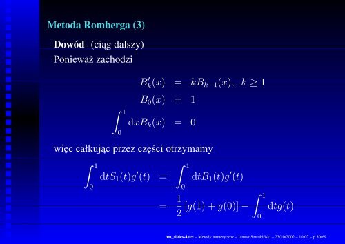
Metoda Romberga (3)<br />
Dowód (ciąg dalszy)<br />
Ponieważ zachodzi<br />
B k(x) ′ = kB k−1 (x), k ≥ 1<br />
∫ 1<br />
0<br />
B 0 (x) = 1<br />
dxB k (x) = 0<br />
więc całkując przez części otrzymamy<br />
∫ 1<br />
0<br />
dtS 1 (t)g ′ (t) =<br />
∫ 1<br />
0<br />
dtB 1 (t)g ′ (t)<br />
= 1 2 [g(1) + g(0)] − ∫ 1<br />
0<br />
dtg(t)<br />
nm_slides-4.tex – <strong>Metody</strong> <strong>numeryczne</strong> – Janusz Szwabiński – 23/10/2002 – 10:07 – p.30/69