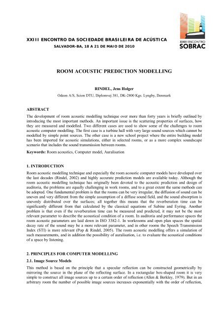
ROOM ACOUSTIC PREDICTION MODELLING - Odeon

XXIII ENCONTRO DA SOCIEDADE BRASILEIRA DE ACÚSTICA
ABSTRACT
SALVADOR-BA, 18 A 21 DE MAIO DE 2010
ROOM ACOUSTIC PREDICTION MODELLING
RINDEL, Jens Holger
Odeon A/S, Scion DTU, Diplomvej 381, DK-2800 Kgs. Lyngby, Denmark
The development of room acoustic modelling technique over more than forty years is briefly outlined by
introducing the most important methods. An important issue is the scattering properties of surfaces, how
they are measured and modelled. Two different cases are used to show some of the challenges to room
acoustic computer modelling. The first case is a turbine hall with very large sound sources which cannot be
modelled by simple point sources. The other case is a new school project where the entire building model
has been imported for acoustic simulations, either in selected rooms, or as a more complex soundscape
scenario that includes the sound transmission between rooms.
Keywords: Room acoustics, Computer model, Auralisation
1. INTRODUCTION
Room acoustic modelling technique and especially the room acoustic computer models have developed over
the last decades (Rindel, 2002) and highly accurate prediction models are available today. Although the
room acoustic modelling technique has originally been devoted to the acoustic prediction and design of
auditoria, the problems are equally challenging in work rooms, and to a great extent the same methods can
be adopted. One fundamental problem is that the rooms can be very irregular, the diffusion of sound can be
uneven and very different from the simple assumption of a diffuse sound field, and the sound absorption is
unevenly distributed over the surfaces; all together this means that the reverberation time can be
significantly different from that calculated by the classical equations of Sabine and Eyring. Another
problem is that even if the reverberation time can be measured and predicted, it may not be the most
relevant parameter to describe the acoustical condition of a room. In auditoria and performance spaces the
room acoustic parameters are laid down in ISO 3382-1. In workrooms and open plan spaces the spatial
decay rate of the sound may be a more relevant parameter, and in other rooms the Speech Transmission
Index (STI) is more relevant (Pop & Rindel, 2005). The room acoustic modelling offers a simulation of
such measurements, and in addition the possibility of auralisation, i.e. to evaluate the acoustical conditions
of a space by listening.
2. PRINCIPLES FOR COMPUTER MODELLING
2.1. Image Source Models
This method is based on the principle that a specular reflection can be constructed geometrically by
mirroring the source in the plane of the reflecting surface. In a rectangular box-shaped room it is very
simple to construct all image sources up to a certain order of reflection (Allen & Berkley, 1979). But in an
arbitrary room the number of possible image sources increases exponentially with the order of reflection,

and thus the method is not suitable for rooms like concert halls where reflection orders of several hundred
are relevant for the audible reverberant decay.
2.2. Particle racing Models
A more realistic way to simulate the decaying sound is to trace a large number of particles emitted in all
directions from a source point. Each particle carries a certain amount of sound energy that is reduced after
each reflection according to the absorption coefficient of the surface involved. As shown in Fig. 1 the result
is the average decay curve for the room from which the reverberation time is evaluated (Schroeder, 1970).
Figure 1. Particle tracing based on geometrical acoustics. Left: The sound energy follows the path of
several hundred rays (only one is shown), and the energy of the particles is reduced when they hit an
absorbing surface. Right: Average decay curve. (Schroeder, 1970).
2.3. Ray Tracing Models
The first computer model that was used for practical design of auditoria was a ray tracing model (Krokstad
et al., 1968). A large number of sound rays are traced from a source point up to high order reflections
following the geometrical/optical law of reflection. The main result of this early model is the distribution of
ray hits on the audience surface, analysed in appropriate intervals of the time delay. So, this is a qualitative
presentation of the sound distribution in space and time. For a closer analysis the direction of incidence of
each ray can also be indicated. In order to obtain quantitative results it is necessary to introduce receiver
surfaces or volumes for detection of the sound rays. So, an approximate energy-reflectogram can be
calculated and used for an estimate of some room acoustic parameters.
2.4. Cone Tracing Models
An alternative to the receiver volume used in ray tracing models is a point receiver in combination with
cones that have a certain opening angle around the rays. Cones with circular cross section have the problem
of overlap between neighbour cones (Vian & van Maerke, 1986). Cones with a triangular cross section can
solve this problem, but still it is difficult to obtain reliable results with this method.

Figure 2: Tracing of a circular cone from the source S to the receiver M. The first order
(S´) and second order (S´´) image sources are also shown. (Vian & van Maerke, 1986).
2.5. Radiosity Models
The principle is that the reflected sound from a surface is represented by a large number of source points
covering the surface and radiating according to some directivity pattern, typically a random distribution of
directions (Lewers, 1993). This method has also been used as an efficient way to model the scattered part
of the early reflected sound.
2.6. Hybrid Models
The disadvantages of the classical methods have lead to development of hybrid models, which combine the
best features of two or more methods. Thus modern computer models can create reliable results with only
modest calculation times. The inclusion of scattering effects and angle dependent reflection with phase
shifts has made it possible to calculate impulse responses with a high degree of realism. This in turn has
been combined with Head Related Transfer Functions (HRTF) to give Binaural Room Impulse Responses
(BRIR), which are convolved with anechoic sound recordings to make auralisation of high quality.
A hybrid model is used in Odeon for the calculation of late reflections. The rays are treated as carriers of
energy and each time a ray hits a surface, a secondary source is generated at the collision point, see Fig. 3,
left side. The energy of the secondary source is the total energy of the primary source divided by the
number of rays and multiplied by the reflection coefficients of the surfaces involved in the ray's history up
to that point. Each secondary source is considered to radiate into a hemisphere with a directivity that may
take the frequency dependent scattering of the surface and the angle of incidence into account. The
contributions from the secondary sources are collected from the receiver position, see Fig. 3, right side. The
time of arrival of a reflection is determined by the sum of the path lengths from the primary source to the
secondary source via intermediate reflecting surfaces plus the distance from the secondary source to the
receiver. A visibility test is made to ensure that a secondary source only contributes a reflection if it is
visible from the receiver. Thus the late reflections are specific to a certain receiver position and it is
possible to take shielding and convex room shapes into account.
Figure 3: Principle of late reflections in Odeon. Left: Secondary sources created on the surfaces by one of the rays in the ray
tracing. Right: A receiver point collects contributions from the visible secondary sources.
3. SCATTERING
3.1. Scattering due to surface roughness
Due to the wavelength of sound being comparable to typical dimensions of reflecting surfaces in rooms, the
scattering effects are very important for a room acoustic simulation model. The scattering effects can be
divided into two; the scattering due to the surface roughness, and the scattering due to edges and finite

dimensions of the reflecting surface (Christensen & Rindel, 2005). Both can be described by a frequency
dependent scattering coefficient, ss and sd.
The surface scattering coefficient can be measured at random incidence according to the method laid down
in ISO 17497-1. A circular test specimen is placed on a turntable in a reverberation chamber, see Fig. 4,
and the reverberation time is measured four times (with and without the test specimen, with and without
rotation of the turn table). From the measured reverberation times the scattering coefficient can be derived.
It typically increases with the frequency as shown in Fig. 5. Thus, for practical use it may be sufficient to
assign a single, mid-frequency value for surfaces with high roughness; then the scattering at other
frequencies is assumed automatically.
Figure 4: Measurement of the random incidence scattering coefficient. Left: principle. Right: A 1:5 scale
reverberation room with the measurement setup. (Ref.: Vorländer et al. (2004)).
Figure 5: Frequency dependent scattering coefficients for surfaces with different roughness.
The mid-frequency scattering coefficients are indicated in the right side of the graph.
3.2 Scattering due to surface size and distance
The diffraction related scattering coefficient depends on the surface dimensions, the distance from surface
to source and receiver, and the distance of the geometrical reflection point to the nearest edge of the
surface. It is also frequency dependent, being higher at low frequencies.
It follows from diffraction theory that the scattering from the edges of a finite size panel increases with the
distance from surface to source and receiver. In Odeon the combined scattering effect is called the
reflection based scattering coefficient sr and it is calculated from:

where sd is the scattering coefficient due to diffraction and ss is the scattering coefficient due to surface
roughness.
An example of how the reflection based scattering works is shown in Fig. 6. If a relatively small surface
(e.g. a table) reflects sound from a source close to the surface, there is very little scattering, but when the
source is far away from the surface the scattering is high, in accordance with the diffraction theory.
Figure 1: Reflection based scattering from a small surface; the source is the red dot. Left:
source close to surface. Right: Source far from surface.
3.3. Application of scattering coefficients
In a simplified room model the scattering coefficient of the surfaces representing more complicated
structures, e.g. a floor representing the audience area in an auditorium should be assigned a scattering
coefficient. If a measured scattering coefficient is not available the suggestions in Tab. 1 can be used as a
guideline.
Tabel 1: Suggested mid-frequency scattering coefficients for various structures.
Material
Scattering coefficient at
mid-frequency
Audience area 0.6 – 0.7
Rough building structures, 0.3 – 0.5 m deep 0.4 – 0.5
Bookshelf, with some books 0.3
Brickwork with open joints 0.1 – 0.2
Brickwork, filled joints but not plastered 0.05 – 0.1
Smooth surfaces, general 0.02 – 0.05
Smooth painted concrete 0.005 – 0.02
In room models with a high degree of detail, the scattering effect comes automatically from the structures,
and it may be sufficient to apply a default low scattering coefficient of 0.05 to all surfaces.
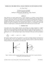
4. CASE 1 – A TURBINE HALL
4.1. Room modelling
sr =
1− ( 1−
sd
) ⋅ ( 1−
ss)
This example is a large turbine hall with the main dimensions: 153 m, 34.5 m, and 20 m. The hall contains
two turbines, one of which is seen on the photo in Fig. 7. A wireframe model of the entire hall is seen in
Fig. 8. It can be noted that the model is much simpler and rough, many details being omitted.

The material data used for the calculations were based on material descriptions and known absorption
coefficients for similar materials and the default scattering coefficient of 0.05 at mid frequencies was
applied to all surfaces.
Figure 7: Turbine hall used as an example of room acoustic modelling.
Fig. 8 shows twelve receiver positions that were used for measuring the sound pressure level in the hall,
and the same positions were used for calculations in the model. A single source position is also shown; this
is used for calculation of the reverberation time and other room acoustic properties in the model as
explained below.
Figure 8: Wireframe model of turbine hall with two turbines roughly modelled. Twelve receiver positions
and a single source position have been inserted.
4.2. Calculation results with a point source
The first question concerning the acoustics of a hall is often the reverberation time, although this may not
be the most appropriate acoustical descriptor in case of large industrial halls. However, even in a very
difficult acoustical environment, i.e. in a room that is far from obeying the assumptions of a diffuse sound
field, a quick and very efficient calculation method for the reverberation time is the so-called global decay.
In principle it is the method of particle tracing originally proposed by (Schroeder, 1970) but further
improved in Odeon with the vector-based scattering method for sound reflections.
Instead of the reverberation time (Ondet & Sueur, 1995) found that the slope of the spatial decay curve
calculated with a single omni-directional sound source could provide a better basis for an acoustical
evaluation in typical non-diffuse work rooms. This method has been described in detail in ISO 14257, and

with a computer model it is simple to simulate this measurement procedure. Using the point source and the
12 receiver positions in Fig. 8 the calculated spatial decay is shown in Fig. 10.
Figure 9: Global decay curves calculated for eight octave bands. The derived reverberation
times for a 30 dB evaluation range are listed in the box to the right
Figure 10: The spatial decay curve calculated for the omni-directional source and the 12 receivers shown
in Fig. 8. The frequency averaged slope is DL2 = 3.53 dB per distance doubling.
4.3. Modelling large noise sources
In work rooms and industrial halls the typical noise sources are big and complicated. Thus, for a good
simulation it is not possible to use only point sources, as usual in auditorium acoustics. Instead the
geometry of the noise sources should be approximately modelled, and the surfaces should be used as
sources radiating sound. In Fig. 11 is shown how one of the turbines has been modelled using 17 surface
sources and two point sources. In this example the radiated sound power was measured using intensity
measuring technique, so each surface in the model could be assigned a certain radiated sound power in
octave bands. Further details are given in (Christensen & Foged, 1998).

Figure 11: One of the turbines modelled by 17 surface sources and 2 point sources. Each source is
assigned a sound power level in octave bands.
4.4. Calculation results with large noise sources
The A-weighted sound pressure had previously been measured in the turbine hall in the 12 positions shown
in Fig. 8. A similar calculation was made with the computer model using in total 34 surface sources and
four point sources. The calculation results are compared to the measured results in Fig. 12, and good
agreement can be observed. The average difference is 0.3 dB and the maximum deviation is 2.2 dB in
position 12.
Figure 12: Comparison of calculated and measured A-weighted sound pressure levels in
12 receiver positions.
One very useful feature of a room acoustic computer model is the possibility to calculate the sound
pressure level in a large number of receiver positions and display the result in a grid map as shown in the
example Fig. 13. In this case with 38 sources and 5202 receivers the calculation time is several hours, so
this kind of calculations are typically made over night.

Figure 13: Mapping of the A-weighted sound pressure level with both turbines active.
The grid size is 1 m and the height is 1.5 m above the floor.
5. CASE 3 – A HIGH SCHOOL WITH OPEN PLAN DESIGN
5.1. Import of the building model
This example is a project for a high school in Denmark, see Fig. 14. In this case it was possible to have
access to the architect’s very detailed 3D model. However, it is questionable which degree of detail is
necessary for a good acoustical simulation; too many details may even make the model less useful for the
acoustic purpose.
Figure 14: Wireframe picture of the room model as imported in Odeon. Total dimensions are 54,4 *
54,4 * 34,1 m. The model has 36 585 surfaces and 15 layers shown in different colours.

For the import of models, e.g. in the dxf interchange format or the 3ds format, Odeon has a very efficient
import function, which automatically can make geometrical checks and an intelligent reduction of the
number of surfaces by gluing triangles and rectangles that define parts of the same surface and creating
polygons instead.
Another challenge to the acoustic modelling is the fact that the architect’s model covers the entire building.
This means that the digital model can be extremely large in terms of the number of surfaces, and it may be
difficult to extract the parts necessary for the acoustical simulation of a particular room in the building.
After import to Odeon and the automatic gluing of surfaces, the model contains 36 585 surfaces. The
import from the dxf file has been highly optimised, but still it takes several minutes.
When the geometry of the model is ready the material properties (absorption and scattering) has to be
assigned to the surfaces. In this process it is a very big advantage if the model has been made with the use
of layers. Typically the layers refer to different materials, and when this is the case, it is possible to assign
the right material properties to all surfaces in a particular layer in one single stroke.
5.2. Calculations
The calculation method used in Odeon for late reflections as described in section 2.6 is very efficient when
it comes to complicated room geometries with remote receiver positions.
To achieve good results it is recommended to look at the reflection density in the calculated impulse
response; it is suggested that the reflection density should be at least 50 per ms. If the reflection density is
too small the calculated decay curve will be far from smooth and thus the calculated room acoustic
parameters will have a relatively high uncertainty. For a calculation to a remote receiver position with no
direct sound and no first order reflections, it is important to include as many details as possible in the late
part of the impulse response and it may be necessary to increase the number of rays. In Table 2 is shown
results obtained with four different calculations, the number of rays ranging from 4000 to 500000.
Table 2: Calculation times and some room acoustical parameters calculated with different number of
rays for a single source and a remote receiver position.
Number of rays 4 000 20 000 100 000 500 000
Calculation time (mm:ss) 00:06 00:24 02:03 10:40
Reflection density (per ms) 20 100 500 2 500
EDT at 1kHz (s) 2.82 2.15 2.29 2.40
T30 at 1kHz (s) 1.29 1.75 1.65 1.66
SPL, dB(A) 32.9 33.8 33.3 33.1
STI 0.37 0.38 0.34 0.36
Some parameters like SPL and STI are not very sensitive to the quality in the impulse response calculation,
as these only need a small reflection density to be determined. Other parameters like EDT and especially
the reverberation time T30 are more sensitive to the reflection density. Obviously 4000 rays are not
sufficient, but already with 20000 rays the decay curves look reasonably smooth. Very little is gained with
more than 100000 rays. For the STI parameter it should be mentioned, that in these calculations the
background noise was not included. This could easily be included in the calculations with the sufficient
information about the background noise level and spectrum.

5.3. Auralisation scenario
In open plan spaces with multiple activities it is often the case that acoustics cannot be settled within the
usual requirements. Sometimes new solutions and new ways of learning and working are inherent in design
of a building. The best way to achieve a mutual understanding of the acoustics of a new design may be by
presenting an auralisation scenario representing various sources in a soundscape including typical activities
within the building. This was done in the described school project and as a result it was decided already in
the design phase to apply an additional amount of sound absorption materials to selected wall surfaces.
Figure 15: Section of the model showing the sources and receiver positions used for the
auralisation scenario.
A scenario for auralisation may include many sound sources. In order to demonstrate the principles an
example with only three sources has been chosen; a nearby person talking, noise from the canteen area on a
different floor in the building, and sound from loud music being transmitted through a wall from the
adjacent classroom, see Fig. 15. Three different listener positions have been chosen. For each listener
position a mix is made from the single auralisations from each of the sources.
The wall consists of glass, gypsum board and a door. The extension of the room acoustic calculation
method to include sound transmission between rooms has been described in detail elsewhere (Rindel &
Christensen, 2008).
6. CONCLUSION
The main reasons for developing room acoustical computer models have been (1) that the assumption of a
diffuse sound field is not fulfilled and thus the classical reverberation equations are not reliable, and (2) in
many rooms other parameters than reverberation time have proven to be important, and such parameters
can only be derived from measurements or computer simulations. In addition the computer models offer
tools for 3D analysis of sound reflections, for mapping of sound distribution, and for auralisation. The
latter has become a useful supplement to the graphs and figures for the acoustic consultant, especially in
the dialogue with architects and building owners about the acoustic solutions for the design of a new
building.

In recent years there has been a development of computer based 3D modelling tools for architectural
design, and thus there has been an increasing demand for efficient interface between the architects’ models
and the acoustical models. Great efforts have been made to meet this demand as demonstrated in the second
case above.
Originally room acoustic computer models have mainly been applied for concert halls and other important
auditoria, in place of - or as a supplement to scale model investigations. Today the computer models are
widely used for all kinds of rooms such as industrial halls, music studios, classrooms and school buildings,
open plan offices, PA-systems for public buildings, sports facilities, train wagons, ships, off shore
facilities, and much more.
REFERENCES
1. Allen, J. & Berkley, D.A. (1979). Image method for efficiently simulating small-room acoustics. J. Acoust.
Soc. Am. 65, 943-950.
2. Christensen, C.L. & Foged, H.T. (1998). A room acoustical computer model for industrial environments - the
model and its verification. Proceedings of Euro-noise 98, München, Germany, 671-676.
3. Christensen, C.L. & Rindel, J.H. (2005). A new scattering method that combines roughness and diffraction
effects. Proceeding of Forum Acusticum, Budapest, Hungary, 2159-2164.
4. ISO 3382-1:2009. Acoustics - Measurement of room acoustic parameters - Part 1: Performance spaces.
5. ISO 14257:2001. Acoustics - Measurement and parametric description of spatial sound distribution curves in
workrooms for evaluation of their acoustical performance.
6. ISO 17497-1:2004. Acoustics - Sound-scattering properties of surfaces - Part 1: Measurement of the randomincidence
scattering coefficient in a reverberation room.
7. Krokstad, A. Ström, S. & Sörsdal, S. (1968). Calculating the Acoustical Room Response by the use of a Ray
Tracing Technique. J. Sound and Vibration 8, 118-125.
8. Lewers, T. (1993). A Combined Beam Tracing and Radiant Exchange Computer Model of Room Acoustics.
Applied Acoustics 38, 161-178.
9. Ondet, A.M. & Sueur, J. (1995). Development and validation of a criterion for assessing the acoustic
performance of industrial rooms. J. Acoust. Soc. Am. 97, 1727-1731.
10. Pop, C.B. & J.H. Rindel, J.H. (2005). Perceived Speech Privacy in Computer Simulated Open-plan Offices.
Proceedings of Inter-noise 2005. Rio de Janeiro, Brazil.
11. Rindel, J.H. (2002). Modelling in Auditorium Acoustics. From Ripple Tank and Scale Models to Computer
Simulations. Revista de Acústica, Vol. XXXIII No 3-4, 31-35.
12. Rindel, J.H. & Christensen, C.L. (2008). Modelling Airborne Sound Transmission between Coupled Rooms.
Proceedings of BNAM 2008, Joint Baltic-Nordic Acoustics Meeting, Reykjavik, Iceland.
13. Schroeder, M.R. (1970). Digital Simulation of Sound Transmission in Reverberant Spaces. J. Acoust. Soc.
Am. 47, 424-431.
14. Vian, J.P. & van Maercke, D. (1986). Calculation of the room impulse response using a ray-tracing method.
Proceedings of 12 th ICA Symposium, Vancouver, Canada, 74-78.
15. Vorländer, M., Embrechts, J.J., De Geetere, L., Vermeir, G. & de Avelar Gomes, M.H. (2004). Case
Studies in Measurement of Random Incidence Scattering Coefficients. Acta Acustica/Acustica 90,
858-867.