Event Study

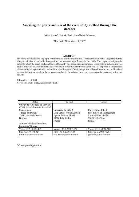
Assessing the power and size of the event study method through the
decades
Nihat Aktas*, Eric de Bodt, Jean-Gabriel Cousin
This draft: November 18, 2007
ABSTRACT
The idiosyncratic risk is a key input to the standard event-study method. The recent literature has suggested that the
idiosyncratic risk is not stable through time, but increased significantly in the 1990s. This paper investigates the
extent to which the event-study method is affected by this economic phenomenon. Using both simulation and real
dataset analyses, we show that classical event-study methods suffer from a significant loss of power in the presence
of increasing idiosyncratic risk, as intuition would suggest. One (perhaps, the only) solution to this problem is to
increase the sample size by a factor corresponding to the ratio of the average idiosyncratic variances in the two
periods.
JEL codes: G14, G34
Keywords: Event Study, Idiosyncratic Risk
Aktas de Bodt Cousin
Université catholique de Louvain
CORE & IAG Louvain School of
Management
1 place des Doyens
1348 Louvain-la-Neuve
Belgium
Université de Lille 2
Lille School of Management
1 place Déliot - BP381
59020 Lille Cédex
France
Université de Lille 2
Lille School of Management
1 place Déliot - BP381
59020 Lille Cédex
France
Academic Fellow Europlace
Institute of Finance
Voice: +32-10-478-439 Voice: +33-3-2090-7477 Voice: +33-3-2090-7477
Fax: +32-10-478-324 Fax: +33-3-2090-7629 Fax: +33-3-2090-7629
nihat.aktas@uclouvain.be eric.debodt@univ-lille2.fr jgcousin@univ-lille2.fr
*Corresponding author.

Fama, Fisher, Jensen and Roll (1969) (referred to below as FFJR) established the foundations of the
(short-term) event-study method, which has become a main tool for empirical research in finance and
accounting. From a method to test the efficient-market hypothesis, to a valuation tool to measure the
wealth effects of corporate events (assuming market efficiency), countless applications have been
published. According to Kothari and Warner (2007), between 1974 and 2000, some 565 papers in
leading finance journals contained an event study 1 .
From a methodological point of view, the literature includes many proposed improvements to the standard
event-study method. Without being exhaustive, the main methodological contributions are the following:
Brown and Warner (1980; 1985) assessed the specification and power of several modifications of the
FFJR approach; Malatesta and Thompson (1985) proposed a model to deal with partially anticipated
events; Ball and Torous (1988) explicitly took into account the uncertainty about event dates; Corrado
(1989) and Cowan (1992) introduced a non-parametric test of significance. Boehmer et al. (1991)
proposed an adaptation of the standard methodology to tackle an event-induced increase in return
volatility; Salinger (1992) suggested an adjustment of the abnormal returns standard errors robust to event
clustering; Savickas (2003) recommended the use of a GARCH specification to control for the effect of
time-varying conditional volatility; Aktas et al. (2004) advocated the use of a bootstrap method as an
alternative to Salinger’s (1992) proposition; Harrington and Shrider (2007) argued that all events induce
variance, and therefore tests robust to cross-sectional variance change should always be used; and
recently, Aktas et al. (2007) proposed a two-state market-model approach to tackle estimation window
contamination.
However, in general, as stressed by Kothari and Warner (2007), the key feature of the event study
approach is its robustness to specific methodological choices (the return-generating model, the statistical
1 The journals surveyed were Journal of Business, Journal of Finance, Journal of Financial Economics, Journal of
Financial and Quantitative Analysis and Review of Financial Studies. Survey and methodological papers are
excluded from the count. Since many academic and practitioner-oriented journals were excluded, the reported figure
provides a lower bound on the size of the event-study literature.
2

test, the length of the estimation and event windows etc.). Thus, except for its reliance on market
efficiency, the event study method appears not to suffer from serious criticisms.
One of the key inputs in calculating the test statistic in an event study is the individual firm (abnormal)
return variance or standard deviation. With respect to this important variable, Kothari and Warner (2007)
report that the mean daily standard deviation for all CRSP listed firms is 0.053 from 1990 to 2002. This is
higher than the value of 0.026 reported by Brown and Warner (1985). Consistent with Campbell et al.’s
(2001) finding, this result implies that individual stocks have become more volatile over time 2 , suggesting
that ‘the power to detect abnormal performance for events over 1990−2002 is lower than for earlier
periods’ (Kothari and Warner, 2007, p. 16). Campbell et al. (2001) also recognised that the increase in the
idiosyncratic volatility might potentially affect the event study analysis. In particular, the authors
emphasise that ‘firm-level volatility is important in event studies. Events affect individual stocks, and the
statistical significance of abnormal event-related returns is determined by the volatility of individual stock
returns relative to the market or industry’ (Campbell et al., 2001, p. 2).
Comparisons of event-study results obtained during different time periods are quite frequent in the
academic literature. As an illustration, we take the case of European mergers and acquisitions (M&A) and
report the results of an event study realized by Goergen and Renneboog (2004). In their Table 11, the
authors provide bidders’ average CARs for the time periods before and after 1999. Before 1999, for a
sample of 74 bidders, the average CAR over the event window [−2,+2] was 1.22% with a t-statistic of
2.98. After 1999, for a sample size of 68 firms, the corresponding average CAR was 1.14% with a t-
statistic of 1.80. Despite the similar CAR levels and sample sizes in the two periods, the statistical
significance is lower in the more recent period. The associated t-statistic is divided by a factor of 1.66.
The loss of power is most likely due to an increase in the idiosyncratic volatility between the two periods.
2 Investigating the period between 1962 and 1997, Campbell et al. (2001) showed that the idiosyncratic risk
increased over time. This result is robust to the model chosen to estimate the idiosyncratic variance, and
economically significant with the firm-level idiosyncratic volatility more than doubling during the period being
analysed.
3

We propose to explore this issue in this paper. More precisely, we investigate whether, and to what extent,
the increase in individual firm’s idiosyncratic volatility affects the power and specification of event
studies. The question is important. If the power and specification of the tests are not stable through time
and/or across geographical zones, it means that comparisons of results obtained from different time
periods and/or geographical zones are potentially biased 3 . It would be like trying to compare the size of
objects using a time varying measurement tool!
We rely on both simulation and real data set analyses. First, we realize a simulation analysis following the
procedure introduced by Brown and Warner (1980. 1985), in which our sample encompasses companies
included in the CRSP daily returns file from 1 January 1976 to 31 December 2004. We simulate both
deterministic and stochastic abnormal returns on the event date. Then, we perform event study analyses on
a real data set of corporate events to check whether the significance tests are affected by a change in
idiosyncratic volatility. The chosen event is a merger and acquisition (M&A) announcement. Our M&A
sample contains 5,401 deals realized by US companies between 1980 and 2004. Our main results are:
― While the specification of the event study is robust to the variation of the idiosyncratic volatility,
we clearly confirm, as expected, a time-variation in the power over the long run. We provide
evidence spanning the period 1976 to 2004 and using the main US stock markets (NYSE, Amex
and Nasdaq). The effect appears to be significant. For example, using the market model and
Boehmer et al.’s (1991) statistical test procedure on a sample of 50 firms, 1% simulated abnormal
returns (with event-induced variance) are detected 74% of the time during the period 1976−1980,
but only 51% of the time during the period 1996−2000.
― We also show that the use of different return-generating models (the constant mean-return model,
the beta-one model and the market model) and/or different statistical test procedures (Brown and
3 Guo and Savickas (in press) show that the level of the average idiosyncratic volatility is different across
geographical zones. For example, over the period 1973 to 2003, the average idiosyncratic volatilities in the UK and
France are less than the half of that in the US.
4

Warner (1980), Boehmer et al. (1991) and the rank test suggested by Corrado (1989)) does not
help to resolve the issue.
― We then confirm these conclusions using a sample of M&A announcements. For example, the
Boehmer et al. (1991) event study approach is far less powerful when the environment is
characterized by a high level of idiosyncratic volatility. The power of the test goes from 98.30%
in 1980-1990 to 21.90% in 1991-2000, with the latter period being the one with the highest level
of idiosyncratic volatility.
― We finally conclude that a practical solution is to increase the sample size to compensate for the
increase in idiosyncratic volatility. To keep the power of the event study constant, a simple rule
of thumb is to increase the sample size by a factor corresponding to the ratio of the average
idiosyncratic variances in the periods being analysed. We provide a two-entry table to facilitate
inter-temporal comparison of event-study results within the US. Using the results provided by
Guo and Savickas (in press), we also present a two-entry table for comparisons of international
event-study results.
This paper is organised in four sections. In Section 1, we show that we must indeed expect that the power
of event studies will be affected by the level of idiosyncratic volatility. Section 2 introduces the research
design. Section 3 is devoted to the presentation of our empirical results based on simulation and real
dataset analyses. The final section summarises our work and presents our conclusions.
1. Econometric arguments
An elegant framework to explore the effects of an increase in firm-level idiosyncratic volatility on the
power and specification of the event-study approach is the dummy-variable regression model introduced
by Karafiath (1988):
R i,
t α i + βi
Rm,
t + γ iDi
, t + ε i,
t
= , (1)
5

where Ri,t and Rm,t are the returns of firm i and of a market-portfolio proxy at time t, respectively. We
identify the event dates using a dummy variable, denoted Di,t, which takes the value 1 for days in the
event window and 0 otherwise. The coefficient of interest, γi, is an estimate of the firm i’s average
abnormal return over the event window (AARi,E).
Under the classical assumptions of identically and independently distributed disturbances εi,t, the standard
regression results provide us with the standard errors of AARi,E:
−1
2
( [ X ' X ] ) σ ( ε )
2
σ ( γ ) = , (2)
i
2,
2
i
where [X'X] −1 corresponds to the inverse of the variance-covariance matrix of the independent variables
and (.)2,2 is the element of the matrix between parentheses located at Row 2 and Column 2. σ 2 (εi) is a
measure of the firm i’s idiosyncratic risk 4 . The effect of an increase in idiosyncratic risk on the variance of
AARi,E is therefore given by:
2
σ ( γ i )
= 2
∂σ
( ε )
1 ( [ X ' X ] ) > 0
∂ −
i
2,
2
. (3)
Equation (3) is strictly positive (it is a variance), which shows that an increase in the idiosyncratic
variance increases the variance of AARi,E. Consequently, this reduces the significance of the coefficient γi.
Therefore, Equation (3) clearly indicates a loss of power due to an increase in a firm’s idiosyncratic risk ,
in a case-study analysis.
For a sample study, we need to compute a statistical test of significance for the cross-sectional average
cumulative abnormal return (ACAR). A convenient candidate is the classical Brown and Warner (1980)
test of significance. Using N to denote the sample size and TE for the length of the event window, the
statistical test of significance for ACAR is given by the Student t-statistic
4 Note that this measure is different from that used by Campbell et al. (2001). These authors introduced a model-free
measure of idiosyncratic risk into their study to avoid the risk of their results being dependent on a specific model.
6

t
ACAR
N
N
1
2 1 2⎛
⎞
= ∑TEγ
i TE
σ ⎜∑
γ i ⎟ . (4)
2
N i=
1
N ⎝ i=
1 ⎠
Using basic algebra to simplify Equation (4), and assuming cross-sectionally uncorrelated cumulative
abnormal returns, the Student t-statistic for the ACAR becomes
where
N
∑
i=
1
γ i
1
t ACAR = , (5)
N σ
2
γ
2
σ γ is the cross-sectional average of the abnormal return variance. Since an increase in
idiosyncratic variance leads to an increase in σ 2 2
(γi), σ γ also increases as the idiosyncratic variance
increases.
Using Equation (5), it is straightforward to show that:
― for value-creating events (positive average abnormal returns), the relation between tACAR and σ
is negative. An increase in firm-level idiosyncratic risk leads to a decrease in the (positive)
Student t-statistic.
― for value-destroying events (negative average abnormal returns), the relation between tACAR and
2
σ γ is positive. An increase in firm-level idiosyncratic risk leads to an increase in the (negative)
Student t-statistic.
To sum-up, we can expect the power of the event-study test to be a decreasing function of the individual
firm’s idiosyncratic risk. We now turn to a systematic exploration of the relationship between
idiosyncratic volatility and event-study power and size, using simulation and real data analyses.
7
2
γ

2. Research design
2.1. Return-generating processes and statistical tests
The abnormal return, ARi,t, corresponds to the forecast errors of a specific normal return-generating model
(in Section 1, to simplify the exposition, we described them as the coefficient estimates of a dummy
variable). In other words, the abnormal return is the difference between the return conditional on the event
and the expected return unconditional on the event. To study the extent to which variations in the
idiosyncratic risk affect the power and size of the event study methods, we used three normal return-
generating processes and three statistical tests. The set of approaches was chosen because they had been
used in classical methodological studies (e.g., Brown and Warner 1980; 1985; Boehmer et al. 1991).
The models of normal returns we considered are the market model (MM), the beta-one model (BETA-1)
and the constant mean return model (CMRM). We selected the MM because it is by far the most
frequently-used model in the literature. The BETA-one model has recently been employed in several
large-scale empirical studies of M&As (Fuller et al. 2002; Moeller et al. 2004; 2005) to avoid using data
from an estimation window which itself contains other M&A deal announcements. We selected the
CMRM because its simplicity might indicate some robustness to a noisy environment. Using the same
notation as in Section 1 (the hat and the bar symbols are used to denote, respectively, coefficient estimates
and sample averages from estimation-window data), we compute the abnormal return for stock i at time t
using the three equations:
(MM) AR = R − ˆ α + ˆ β R ) ; (6)
i,
t i,
t ( i i m,
t
(BETA-1) i t = Ri
t − Rm
t ; (7)
AR , , ,
(CMRM) ARi, t = Ri,
t − Ri
. (8)
We used three statistical tests: the Brown and Warner (1980) test (BW), the Boehmer et al. (1991) test
(BMP), and the Corrado (1989) rank test (RANK). These are probably the tests most regularly used in the
8

academic literature. Let us denote by N the number of firms in the dataset, by T the number of days in the
estimation window, by E the event date, by σi the standard deviation of firm i’s abnormal returns during
the estimation window, and by Rm,t the market return for day t. The three statistical tests are defined in
Equations (9), (11) and (12).
The BW test is also known as the traditional method. It implicitly assumes that the security residuals are
uncorrelated and that event-induced variance is insignificant. The test statistic is the sum of the event-
induced returns divided by the square root of the sum of all the securities’ estimation-window residual
variances:
BW
=
1
N
N
∑
i=
1
1
N
AR
N
∑
2
i=
1
i,
E
σ
2
i
. (9)
The second test we adopted is the BMP test which is a cross-sectional approach relying on the use of
standardised abnormal returns. To compute the test statistic, we need first to compute the standardised
abnormal return of firm i on the event date (SRi,E):
SR
i,
E
= AR
i,
E
The BMP test statistic is then
BMP =
1
N(N −1)
⎡
⎤
⎢
2
1 (R ⎥
m,
E − Rm
)
⎢σ
+ +
⎥
i 1
T
. (10)
⎢ T
2 ⎥
⎢ ∑ (Rm,t
− Rm
)
⎥
⎣
t=
1
⎦
1
N
N
N
∑
i=
1
SR
i,
E
N
∑(SRi , E −∑
i=
1 i=
1
SR
i,
E
N
9
)
2
. (11)

The BMP test was introduced to deal with event-induced variance. At first sight, the BMP test should be
more robust to idiosyncratic-risk variations than the BW test, because firm-level residual volatility is only
use to standardise the abnormal return. Indeed, assuming homoscedasticity, it is straightforward to show
that the BMP test is independent of the level of the idiosyncratic risk (see Appendix for a formal proof).
The last test we chose is the one introduced by Corrado (1989). It is a non-parametric test based on the
ranks of abnormal returns. The RANK test merges the estimation and event windows in a single time
series. Abnormal returns are sorted and a rank is assigned to each day. If Kj,t is the rank assigned to firm
i’s abnormal return on day t, then the RANK test is given by
RANK
1
N
=
N
∑
i=1
(K
S(K)
iE −
K)
, (12)
where K is the average rank and SE(K) is the standard error, calculated as
+ 1 1 1
2
= ∑ ∑ −
+ 1
T N
SE(K) ( (Kit
K))
. (13)
T N
t=
1 i=
1
The use of ranks neutralises the impact of the shape of the AR distribution (including its skewness and
kurtosis, and the presence of outliers). It should therefore represent an attractive alternative way of dealing
with changes in idiosyncratic risk.
2.2. Simulations
Our investigation of the specification and power of the event study methods to a change in firm-level
idiosyncratic risk follows the procedure introduced by Brown and Warner (1980; 1985) and used
repeatedly since then (see, e.g., Corrado, 1989; Boehmer et al. , 1991; Corrado and Zivney, 1992; Cowan,
1992; Cowan and Sergeant, 1996; Savickas, 2003; Aktas et al. 2007).
10

Sample construction. Our universe of firms is composed of companies included in the CRSP daily returns
file from 1 January 1976 to 31 December 2004. We divide this 29-year period into 6 non-overlapping sub-
periods (1976−1980, 1981−1985, 1986−1990, 1991−2000 and 2001−2004). As our market portfolio we
used the CRSP equally weighted index. All firms and event dates were randomly chosen with replacement
such that each firm/date combination had an equal chance of being chosen at each selection. For each
replication, we constructed 1,000 samples of N firms (N being equal to 50, 100, 150 and 200,
respectively). The estimation window length was 200 days and the event date was situated at day 206.
Like Savickas (2003), our sampling process excluded securities with missing returns during the 206-day
interval. Moreover, to be included in the samples, securities needed to have at least 100 non-zero returns
over the estimation window, and not to have a zero return due to a ‘reported price’ on the event-day.
Abnormal performance simulation. We generated abnormal returns at the event date in the same way as
Brown and Warner (1980; 1985) by adding a constant to each stock return observed on day 0 (event date).
The abnormal performance simulated (ARi,E) is 0% for the specification analysis and +1% for the power
analysis. These shocks are either deterministic or stochastic. To simulate the event-induced variance
phenomenon for stochastic shocks, each security’s event-day return (Ri,E) was transformed to triple its
variance by adding two de-meaned returns randomly drawn from the estimation window. The event-day
transformed return was therefore obtained using the equation
R = R + AR + ( R − R ) + + ( R − R ) , (14)
' i,
E i,
E i,
E i,
X i
i,
Y i
where Ri,X and Ri,Y are the two randomly drawn returns from the estimation window.
2.3. Some descriptive statistics
Table 1 displays some descriptive statistics for the universe of stocks used in the simulation analyses in
the six sub-periods. Panel A presents the number of stocks for the all-US universe (NYSE, Amex and
Nasdaq) and for the NYSE-Amex and Nasdaq sub-samples. Unsurprisingly, starting from the mid-1980s,
the number of stocks listed on the Nasdaq is higher than the number of stocks listed on the NYSE-Amex.
Panel B shows average market values (median values are reported in italics). Even allowing for the fact
11

that these numbers are not adjusted for inflation, they confirm the significant growth in the average
market value of listed stocks and, for each sub-period, the huge difference in average market values of
stocks listed on the NYSE-Amex and those listed on the Nasdaq. Moreover, the difference between the
average and median market values suggests the presence of a few large firms in each of these universes.
Another observation worth mentioning is that the size differential between medians of the NYSE-Amex
and Nasdaq stocks decreases slightly (the ratio of the NYSE-Amex median market value to the Nasdaq
median market value goes from 0.16 in the 1976−1980 sub-period to 0.28 in the 2000−2004 sub-period).
Panel C presents some information on market risk (MR) and the average idiosyncratic risk (IR). The
market risk for a given sub-period (of length T days) is computed as
MR = σ ( Rm
) , (15)
where, σ(Rm) is the standard deviation over the sub-period of the CRSP equally weighted index daily
return. The idiosyncratic risk for a given stock is given by the standard deviation of the residual of the
MM applied to the stock daily return over the sub-period 5 . The average idiosyncratic risk, for a given sub-
period (of length T days), is simply the average of the individual firm’s idiosyncratic risks, and is given by
N 1
IR = σ ( ε i ) , (16)
N
∑
i=
1
where, N corresponds to the number of listed stocks in the universe. Panel C shows that:
― In the all sub-periods, the idiosyncratic risk is larger than the market risk.
― Consistent with Campbell et al.’s (2001) results, the IR has been rising through time, almost
doubling between 1976−1980 and 1996−2000sub-periods. This change is clearly due to the
Nasdaq sub-sample of stocks.
5 Campbell et al. (2001) show that their model-free decomposition procedure gives very similar results.
12

― The most recent sub-period (2000−2004) is however characterised by a decline in IR. This result
is also reported by Brandt et al. (2005). Therefore, it is more appropriate to speak of IR variation
through time than of a systematic rise in IR.
3. Empirical results
3.1. Simulation results
Our simulation results are presented in two tables and one figure. Table 2 is concerned with deterministic
shocks (no event-induced variance), while Table 3 summarises our results for stochastic shocks (event-
induced variance). Each table is divided into two panels. Panel A is devoted to the specification analyses
and Panel B to the power analyses. For the sake of concision, we have limited ourselves to presenting the
results for the analyses with portfolios of 50 and 200 stocks. The results for other portfolio sizes are
presented in Figure 2, for the BMP test only.
Deterministic shocks. Table 2, Panel A shows that the specification seems not to be an issue. Except for
the RANK test combined with the CMRM return-generating process, all the process and statistical test
combinations are well specified for all sub-periods. Concerns about the specification of the RANK test
have already been reported by several authors (Aktas et al., 2007; Cowan and Sergeant, 1996; Serra,
2002; Savickas, 2003). The variation in IR during the period seems not to impact the specification. This,
somewhat unexpected (as the variation in IR might have distorted the shape of the return distribution)
result seems to confirm the robustness of the standard event-study method. However, Table 2, Panel B
presents less encouraging results. They can be summarised as follows:
― With a sample size of 50 stocks, the loss of power of the BW (whatever the chosen return-
generating process) is substantial. For example, with the MM, it falls from 91.6% for the
1976−1980 period to 48.2% for the 1996−2000 period (the period in which the IRs were highest).
13

― The BMP and the RANK tests are less affected by this problem. With a portfolio size of 50
stocks, the percentage of detected AR is always above 80%, whatever return-generating process
is used.
― The comparison between the results obtained with portfolios of 50 stocks and 200 stocks reveals
that an increase in portfolio size solves the loss of power issue that affects the BW test.
Stochastic shocks. Table 3, Panel A repeats the specification exercise for stochastic shocks. The event-
induced variance phenomenon drastically affects the specification of both the BW and the RANK tests,
irrespective of the return-generating process and the portfolio size. Only the BMP test, specifically
designed to tackle this issue, deals with stochastic shocks successfully. With respect to our research
question, we note that there is no clear trend over the sub-periods. The specification issues encountered
with stochastic shocks seem not to be related to the time variation in IRs. With respect to the power of the
tests, Table 3, Panel B highlights two main issues:
― For a portfolio size of 50 stocks, all combinations of statistical test and return-generating process
suffer from a dramatic loss of power. For the 1996−2000 sub-period (which has the highest IR),
the most powerful combination (RANK – MM) detects 62.3% of the simulated abnormal returns.
This compares unfavourably with a detection rate of 94.8% for deterministic shocks. Table 3,
Panel A also reveals specification issues with respect to the RANK – MM pairing.
― Increasing the portfolio size from 50 to 200 stocks alleviates the loss of power. All statistical test
and return-generating process combinations detect more than 80% (and generally more than 90%)
of stochastic ARs.
The clear message delivered by Tables 2 and 3 is that, for both deterministic and stochastic shocks, as
long as the sample size is large enough, the BMP approach is the most robust to a variation in
idiosyncratic risk, in terms of both specification and power. This result does not depend on the return-
generating process used, as already shown by Brown and Warner (1980; 1985).
14

As the portfolio size clearly plays a critical role, we explored its impact on the specification and power of
the BMP test (associated in this specific case with the MM return-generating process) in more depth.
Since the behaviour of the BMP test differs significantly from sub-period to sub-period with respect to the
specification error (see Tables 2 and 3), it is not possible to compare the power of the test across sub-
periods. To overcome this problem, we resorted to a graphical method, the ‘size–power curves’ proposed
by Davidson and MacKinnon (1998) 6 . Using the simulation techniques described in Section 2 above, we
generated a portfolio of stocks of size N. Then, for each portfolio, we computed the power and size of the
BMP test for 100 different theoretical significance levels (between 0% and 100%). The results are
presented in Figure 1, although for clarity we have only shown three different sub-periods there.
The results confirm our previous findings. For a comparable level of specification error, the power of the
BMP test increases with sample size. For all portfolio sizes, the lowest size-power curve is obtained for
the 1996−2000 sub-period (which has the highest average idiosyncratic risk). However, increasing the
sample size dramatically reduces the loss of power produced by an increase in the idiosyncratic risk. The
size-power curves for the three sub-periods are closer to each other in Panel D (200 stocks) than in
Panel B (100 stocks).
3.2. M&A sample
Although the Brown and Warner (1980;1985) simulation procedure is now well-established for exploring
the power and specification of standard event-study methods, it is still interesting to see whether the
results obtained are similar for a real sample of corporate event announcements. In this sub-section we
provide evidence from the M&A field.
To obtain results which can be compared to the previous literature (Travlos, 1987; Fuller et al., 2002), we
focused on large stock-paid deals involving US listed acquirers. Our data on M&As is taken from the
6 Originally, the size–power curves allowed the power of alternative test statistics that did not have the same size
(specification) to be compared. However, we used this graphical method to perform a time-series comparison of the
results with the BMP test.
15

Thompson SDC (securities data company) database; it includes all deals announced during the period
1980−2004 for which the acquirer was a US listed firm, the deal size above USD 50 million, and the
consideration 100% stock. There are 6,500 such deals for which we were able to estimate the acquirer’s
CAR. We computed the abnormal return using the market model (MM) as the return-generating process.
The parameters of the MM were estimated over an estimation window from day −235 to day −11 relative
to the announcement day. We used a 3-day event window (from day −1 to day +1).
Our research design is quite specific at this point. Remember that our goal was to explore whether the
time-variation in idiosyncratic risk affects the power of the standard event-study method using a real
dataset. So, the question here was not whether stock-paid deals by listed acquirers destroy value (a known
result for acquirers of listed targets) but whether, having controlled for the average level of abnormal
returns, the power of the event study varied through time. We proceeded as follows:
― From the initial dataset, we kept only the M&As for which the observed acquirer’s CAR was
between 0 and −2%. This provides us with 5,401 deals with an average CAR (almost by
construction) of around −1%;
― We then divided this dataset into three periods (1980−1990, 1991−2000 and 2001−2004), based
on the announcement day and corresponding to low, high and medium levels of IR respectively
(see Table 1, Panel C). The number of firms in each sub-group was 602, 4,233 and 566 (see
Table 4).
― For each sub-period, we undertook the following simulation experiment: we drew 1,000
portfolios of 50 acquirers, and for each portfolio, we carried out a BMP significance test; finally,
we tracked the frequency with which these portfolios’ average CAR was significant.
This procedure allowed us to control for the expected average CAR (around −1%) by sub-period, and to
directly explore the power of the BMP test during the three time periods. Our results are reported in
Table 4. The row ‘Average 3-day CAR’ shows that our empirical design was successful in keeping the
average CAR of the portfolios approximately constant across sub-periods. The last row shows the
16

frequency with which the average CAR is found to be significant using the BMP test. The drastic impact
of the IR variation through time on the power of the test is confirmed.
3.3. Practical recommendation
In Section 1.2 we quoted some examples from the M&A literature comparing the results of event studies
undertaken at different time period. As a practical recommendation, we would like to present a simple
rule of thumb to compare results from different periods. Let us go back to Equation (9) and denote the two
different time periods (or two different geographical zones), with different levels of average idiosyncratic
risk, by 1 and 2. We obtain the following expressions for the Student t-statistics for the two periods:
t
ACAR , 1
AARE
= and t
1 2
σ ε , 1
N
1
17
ACAR , 2
where AARE is the cross-sectional average abnormal return on the event day and
AARE
= , (17)
1 2
σ ε , 2
N
2
2
σ ε , the cross-sectional
average of the market model residual variance, corresponds to the average idiosyncratic variance.
To allow a fair comparison of results between time periods (or geographical zones), everything else being
constant (in particular, assuming that the level of the wealth impact is the same for the two sub-periods i.e.
AARE,1 = AARE,2), the researcher needs to keep tACAR,2 and tACAR,1 approximately equal. In other words the
condition:
1
σ
N
1
2
ε , 1
1 2
= σ ε , 2
(18)
N
must hold. The rule for comparing results through time emerges naturally, as
σ
σ
2
ε , 2
2
ε , 1
2
N 2 = . (19)
N
1

This means that the ratio of the average idiosyncratic variance between the two time periods (or
geographical zones) must be equal to the ratio of the sample sizes. Table 5, Panel A gives the ratios of the
average idiosyncratic variance in our six non-overlapping sub-periods for the US, as a reference tool for
the reader. These numbers give the ratio of the sample sizes which should be used to allow a fair
comparison of results through time. For example, if the average idiosyncratic variance has doubled, the
sample size should also be doubled. In general, the sample size needs to be multiplied by the ratio of the
idiosyncratic variances. In the same way, Table 5 Panel B displays the ratios of the average idiosyncratic
variance between seven countries. These ratios were computed using the average equal-weighted
idiosyncratic volatility reported by Guo and Savickas (in press). For example, the ratio of the average
idiosyncratic risk in Italy (Average IR = 0.028) and that in Canada (Average IR = 0.139) is 0.20. This
suggests that to have comparable event-study results in terms of power for the same corporate event (e.g.,
an M&A announcement), the Canadian sample needs to include 5 times as many companies as the Italian
sample.
4. Conclusion
Campbell et al. (2001) highlighted the rise in idiosyncratic risk (IR) during the period 1962−1997. The
impact of this observation on the short-term event-study method has not been studied systematically until
now. It raises the question of the extent to which the event-study method is a time-varying measurement
tool. We have investigated this question in this paper. Our two main conclusions are:
― While the specification of Boehmer et al.’s (1991) statistical test is resistant to time variation in
IR, the power of all the event-study approaches investigated here are dramatically affected by the
variation in IR. This result is intuitive: in a noisier environment, detecting abnormal performance
is increasingly difficult.
― A simple solution has emerged from our analysis, which consists of increasing the sample size in
order to compensate for the noise. More specifically, the ratio of sample sizes should be equal to
18

the ratio of idiosyncratic variances to keep the power level of the chosen event-study method
(relatively) constant.
We finally provide, as a reference tool, to allow for unbiased comparison of results published in the
literature, the ratio of idiosyncratic variances through time for the US stock markets and through
geographical zones (for seven countries).
Appendix: Proof that Boehmer et al.’s method is insensitive to idiosyncratic risk change
In this Appendix we prove that Boehmer et al.’s (1991) cross-sectional method (BMP) is not affected by a
change in idiosyncratic risk under conditions of homoscedasticity. Assume that ARi corresponds to the
abnormal return of firm i on the event date and that the variance (σ²) of the market-model residual is the
same for each sample firm (homoscedasticity). The BMP test is implemented in the following way:
― first we standardise the abnormal return by dividing it by its standard deviation:
ARi
SAR i = ;
σ
― the cross-sectional average of the standardised abnormal (ASAR) return is given by
ASAR
N
∑
i=
= 1
N
19
SAR
i
� ASAR =
AAR
σ
where AAR is the cross-sectional average abnormal return, and N is the total number of
firms in the sample;
― the variance of the average standardised abnormal return is
― the t-stat following BMP is given by
2
2 σ SAR
σ ASAR = ; 2
N
AAR
ASAR
t − stat = �
σ
σ ASAR
SAR
N
σ
t
− stat =

� t − stat =
1
σ
N
∑
i=
1
20
AAR
N
σ
( AR − AAR)
i
N −1
2
N.
AAR
= ;
σ
where σAR corresponds to the cross-sectional variance of the abnormal return.
In the homoscedastic case, as defined above, the Student t-statistic is independent of the variance of the
individual firm’s market-model residual.
AR

References
Aktas, N., E. de Bodt and R. Roll, 2004. Market response to European regulation of business
combinations, Journal of Financial and Quantitative Analysis 39, 731–758.
Aktas, N., J.G. Cousin and E. de Bodt, 2007. Event studies with a contaminated estimation period,
Journal of Corporate Finance 13, 129–145.
Ball, C. and W. Torous, 1988. Investigating security-price performance in the presence of event-date
uncertainty, Journal of Financial Economics 22, 123–154.
Brandt, M.W., A. Brav and J.R. Graham, 2005. The idiosyncratic volatility puzzle: time trend or
speculative episodes? SSRN Working Paper: http://ssrn.com/abstract=851505.
Brown, S. and J. Warner, 1980. Measuring security price performance, Journal of Financial Economics 8,
205–258.
Brown, S. and J. Warner, 1985. Using daily stock returns: the case of event studies, Journal of Financial
Economics 14, 3–31.
Boehmer, E., J. Musumeci and A. Poulsen, 1991. Event study methodology under conditions of event
induced variance, Journal of Financial Economics 30, 253–272.
Campbell, J. Y., M. Lettau, B. Malkiel and Y. Xu, 2001. Have individual stocks become more volatile?
An empirical exploration of idiosyncratic risk, Journal of Finance 56, 1−43.
Corrado, C., 1989. A nonparametric test for abnormal security price performance in event studies, Journal
of Financial Economics 23, 385–395.
Corrado, C. and T. Zivney, 1992. The specification and power of the sign test in event study hypothesis
tests using daily stock returns, Journal of Financial and Quantitative Analysis 27, 465–478.
Cowan, A., 1992. Nonparametric event study tests, Review of Quantitative Finance and Accounting 2,
343–358.
Cowan, A. and A. Sergeant, 1996. Trading frequency and event study test specification, Journal of
Banking and Finance 20, 1731−1757.
Davidson, R. and J.G. MacKinnon, 1998, Graphical methods for investigating the size and power of
hypothesis tests, The Manchester School 66, 1−26.
Fama, E., L. Fisher, M. Jensen and R. Roll, 1969. The adjustment of stock prices to new information,
International Economic Review 10, 1–21.
Fuller, K., J. Netter and M. Stegemoller, 2002. What do returns to acquiring firms tell us? Evidence from
firms that make many acquisitions, Journal of Finance 57, 1763−1793.
Goergen, M. and L. Renneboog, 2004. Shareholder wealth effects of European domestic and cross-border
takeover bids, European Financial Management 10, 9−45.
Guo, H. and R. Savickas, (in press). Average idiosyncratic volatility in G7 countries, Review of Financial
Studies.
Harrington, S. and D. Shrider, 2007. All events induce variance: analyzing abnormal returns when effects
vary across firms, Journal of Financial and Quantitative Analysis 42, 229–256.
Karafiath, I., 1988. Using dummy variables in the event methodology, Financial Review 23, 351−357.
Kothari, S.P. and J.B. Warner, 2007. Econometrics of event studies, in Eckbo, B.E. (ed.) Handbook of
Corporate Finance, North Holland Elsevier, pp. 3−36.
Malatesta, P. and R. Thompson, 1985, Partially anticipated events: a model of stock price reactions with
an application to corporate acquisitions, Journal of Financial Economics 14, 237–250.
21

Moeller, S.B., F.P. Schlingemann and R.M. Stulz, 2004. Firm size and the gains from acquisitions,
Journal of Financial Economics 73, 201−228.
Moeller, S.B., F.P. Schlingemann and R.M. Stulz, 2005. Wealth destruction on a massive scale? A study
of acquiring-firm returns in the recent merger wave. Journal of Finance 60, 757−782.
Salinger, M., 1992. Standard errors in event studies, Journal of Financial and Quantitative Analysis 27,
39–53.
Savickas, R., 2003. Event-induced volatility and tests for abnormal performance, Journal of Financial
Research 16, 165–178.
Serra, A.P., 2002. Event study tests: a brief survey. Working Paper FEP, Vol. 117. University of Porto.
Travlos, N.G., 1987. Corporate takeover bids, methods of payment, and bidding firms' stock returns,
Journal of Finance 42, 943−963.
22

Figure 1. Size-power curves for the BMP test
This figure provides size-power curves for Boehmer et al.’s (1991) test (BMP) for different sample sizes (N=50, 100,
150 and 200). We have simulated an event-induced return of 1% and an event-induced increase in return volatility.
Three different sub-periods, with different average idiosyncratic risk (IR) levels are simulated: 1976−1980 low IR;
2001−2004 median IR; and 1996−2000 high IR.
100%
90%
80%
70%
60%
50%
40%
30%
20%
10%
Power
Panel A. N=50
Size
0%
0.0% 2.5% 5.0% 7.5% 10.0% 12.5% 15.0% 17.5% 20.0%
100%
95%
90%
85%
80%
75%
Power
[1976-1980]
Panel B. N=100
[2001-2004]
23
[1976-1980]
[2001-2004]
[1996-2000]
[1996-2000]
Size
70%
0.0% 2.5% 5.0% 7.5% 10.0% 12.5% 15.0% 17.5% 20.0%

100%
95%
90%
85%
80%
75%
Power
[1976-1980]
Panel C. N=150
[2001-2004]
Size
70%
0.0% 2.5% 5.0% 7.5% 10.0% 12.5% 15.0% 17.5% 20.0%
100%
95%
90%
85%
80%
75%
Power
[1976-1980]
[2001-2004]
Panel D. N=200
[1996-2000]
24
[1996-2000]
Size
70%
0.0% 2.5% 5.0% 7.5% 10.0% 12.5% 15.0% 17.5% 20.0%

Table 1. Descriptive statistics
This table presents descriptive statistics for the universe of stocks used for the simulation analyses. We work on six
non-overlapping sub-periods, spanning a time period of 29 years. For each sub-period, we show in Panel A the
number of stocks (for the whole universe and for the NYSE-Amex and Nasdaq sub-samples), in Panel B the average
market value of firms in the corresponding universe (median value are reported in italic), and finally in Panel C,
using the decomposition approach presented in Section 2, the evolution of the average market (MR) and
idiosyncratic (IR) risks.
Panel A. Number of stocks
1976–1980 1981–1985 1986–1990 1991–1995 1996–2000 2001–2004
NYSE–Amex–Nasdaq 2,357 2,531 3,596 4,242 4,724 4,732
NYSE–Amex 1,241 1,259 1,503 1,925 2,131 2,302
Nasdaq 1,116 1,272 2,093 2,317 2,593 2,430
Panel B. Market value
NYSE–Amex–Nasdaq 652,047 742,209 935,073 1,148,800 2,152,303 2,340,279
68,034 99,404 103,990 131,209 192,632 220,288
NYSE–Amex 649,232 939,919 1,411,223 1,782,985 3,389,517 3,888,836
99,651 173,764 232,443 267,256 394,104 453,000
Nasdaq 657,527 281,910 122,892 247,285 855,215 880,718
16,840 29,772 32,461 50,619 102,011 127,656
Panel C. Market and idiosyncratic risks
MR 0.006 0.006 0.007 0.005 0.008 0.009
IR 0.019 0.020 0.026 0.030 0.033 0.030
IR NYSE–Amex 0.018 0.019 0.022 0.022 0.024 0.021
IR Nasdaq 0.021 0.023 0.035 0.043 0.045 0.039
25

Table 2. Rejection rates of test statistics: no event-induced variance
This table presents our simulation results for the six sub-periods with deterministic shocks. The simulation procedure
is described in Section 2. The sample size is N. CMRM, BETA and MM are respectively the constant mean return
model, the beta model and the market model return-generating processes. BW, BMP and RANK refer to the Brown
and Warner (1980), Boehmer et al. (1991) and Corrado’s (1989) tests, respectively. The event-induced return is 0%
for the specification analysis and +1% for the power analysis.
Panel A. Specification
N=50
CMRM
BW
BETA MM CMRM
BMP
BETA MM CMRM
RANK
BETA MM
1976–1980 4.70% 4.70% 5.20% 4.50% 2.80% 3.70% 1.50% 2.30% 2.50%
1981–1985 5.00% 4.90% 4.50% 5.10% 5.80% 4.50% 4.90% 7.00% 5.40%
1986–1990 6.30% 6.90% 6.00% 3.80% 3.80% 4.00% 2.90% 1.80% 1.90%
1991–1995 5.00% 4.20% 5.00% 4.50% 2.50% 4.40% 2.90% 1.40% 1.50%
1996–2000 5.40% 5.30% 5.80% 3.90% 3.90% 4.10% 2.60% 4.10% 2.80%
2001–2004 3.60% 3.80% 4.30% 4.20% 3.00% 4.20% 2.90% 3.50% 3.20%
N=200
CMRM
BW
BETA MM CMRM
BMP
BETA MM CMRM
RANK
BETA MM
1976–1980 7.00% 4.40% 5.70% 3.70% 1.60% 2.30% 66.30% 3.20% 3.80%
1981–1985 5.00% 5.60% 4.30% 3.70% 5.10% 3.90% 51.90% 5.20% 5.30%
1986–1990 6.50% 8.00% 7.20% 4.30% 5.70% 5.40% 30.20% 6.00% 6.70%
1991–1995 4.70% 4.30% 5.10% 4.60% 3.00% 4.80% 24.40% 4.80% 4.20%
1996–2000 4.20% 4.40% 4.80% 4.10% 3.40% 3.90% 9.60% 5.90% 4.80%
2001–2004 5.40% 4.60% 4.10% 6.60% 4.10% 5.30% 6.00% 5.20% 5.20%
Panel B. Power
N=50
CMRM
BW
BETA MM CMRM
BMP
BETA MM CMRM
RANK
BETA MM
1976–1980 89.4% 90.3% 91.6% 98.0% 98.4% 98.8% 99.9% 99.6% 99.6%
1981–1985 86.9% 89.3% 89.1% 96.5% 97.2% 96.9% 99.9% 99.9% 99.9%
1986–1990 56.0% 58.8% 59.0% 84.9% 88.7% 89.3% 97.0% 97.7% 97.7%
1991–1995 49.5% 49.9% 51.3% 87.9% 86.5% 89.2% 96.5% 96.4% 96.3%
1996–2000 44.7% 45.1% 48.2% 85.0% 82.9% 87.1% 93.1% 92.5% 94.8%
2001–2004 57.9% 60.5% 62.7% 93.8% 93.7% 95.2% 98.0% 98.6% 99.1%
N=200
CMRM
BW
BETA MM CMRM
BMP
BETA MM CMRM
RANK
BETA MM
1976–1980 100.0% 100.0% 100.0% 100.0% 100.0% 100.0% 100.0% 100.0% 100.0%
1981–1985 100.0% 100.0% 100.0% 100.0% 100.0% 100.0% 100.0% 100.0% 100.0%
1986–1990 97.5% 98.3% 97.7% 100.0% 100.0% 100.0% 100.0% 100.0% 100.0%
1991–1995 94.8% 94.5% 95.4% 100.0% 100.0% 100.0% 100.0% 100.0% 100.0%
1996–2000 93.9% 95.1% 94.3% 100.0% 100.0% 100.0% 100.0% 100.0% 100.0%
2001–2004 99.8% 99.9% 99.9% 100.0% 100.0% 100.0% 100.0% 100.0% 100.0%
26

Table 3. Rejection rates of test statistics: event–induced variance
This table presents our simulation results for the six sub-periods with deterministic shocks. The simulation procedure
is described in Section 2. The sample size is N. CMRM, BETA and MM are respectively the constant mean return
model, the beta model and the market model return-generating processes. BW, BMP and RANK refer to the Brown
and Warner (1980), Boehmer et al. (1991) and Corrado’s (1989) tests, respectively. The event-induced return is 0%
for the specification analysis and +1% for the power analysis.
Panel A. Specification
N=50
CMRM
BW
BETA MM CMRM
BMP
BETA MM CMRM
RANK
BETA MM
1976–1980 14.80% 14.70% 15.70% 4.80% 3.60% 4.30% 4.90% 5.80% 6.20%
1981–1985 18.00% 17.70% 16.70% 6.50% 6.60% 5.90% 7.80% 7.30% 7.00%
1986–1990 15.70% 16.50% 16.50% 4.00% 4.10% 4.00% 6.20% 7.10% 7.20%
1991–1995 16.60% 15.90% 16.50% 4.70% 3.50% 4.40% 6.00% 7.10% 6.90%
1996–2000 15.10% 15.50% 16.70% 4.10% 4.00% 4.50% 6.20% 6.80% 6.50%
2001–2004 15.70% 15.90% 16.00% 4.80% 4.70% 5.00% 8.50% 7.80% 8.40%
N=200
CMRM
BW
BETA MM CMRM
BMP
BETA MM CMRM
RANK
BETA MM
1976–1980 18.20% 15.70% 17.70% 5.70% 2.90% 4.50% 2.40% 3.80% 2.80%
1981–1985 18.80% 20.50% 19.00% 5.80% 6.40% 5.00% 5.10% 5.40% 4.80%
1986–1990 18.70% 21.40% 20.80% 5.60% 5.40% 5.80% 6.80% 8.10% 7.40%
1991–1995 15.70% 15.00% 16.40% 3.20% 1.70% 3.40% 4.50% 5.50% 4.80%
1996–2000 14.60% 15.70% 15.90% 5.10% 4.10% 5.60% 5.40% 7.00% 6.20%
2001–2004 15.70% 15.60% 15.90% 4.60% 3.60% 4.60% 7.90% 7.10% 7.00%
Panel B. Power
N=50
CMRM
BW
BETA MM CMRM
BMP
BETA MM CMRM
RANK
BETA MM
1976–1980 77.4% 76.4% 77.9% 74.2% 70.2% 73.9% 85.5% 84.3% 84.9%
1981–1985 74.0% 75.3% 75.0% 69.9% 71.4% 69.9% 82.1% 80.7% 81.4%
1986–1990 51.5% 52.8% 52.7% 50.9% 52.0% 53.2% 66.5% 67.2% 67.0%
1991–1995 49.3% 48.7% 49.0% 52.9% 49.0% 53.8% 62.6% 64.2% 64.5%
1996–2000 46.9% 48.6% 48.6% 51.3% 46.5% 51.3% 60.3% 58.6% 62.3%
2001–2004 55.1% 56.7% 58.2% 62.8% 60.8% 64.1% 73.0% 72.9% 76.3%
N=200
CMRM
BW
BETA MM CMRM
BMP
BETA MM CMRM
RANK
BETA MM
1976–1980 99.5% 99.4% 99.4% 99.9% 99.8% 99.9% 100.0% 100.0% 99.9%
1981–1985 98.6% 99.0% 98.5% 99.8% 99.5% 99.5% 99.9% 99.7% 99.8%
1986–1990 87.4% 89.6% 89.5% 96.8% 97.3% 97.4% 99.0% 98.6% 98.8%
1991–1995 83.3% 82.7% 84.4% 97.2% 94.7% 97.6% 98.2% 98.4% 98.3%
1996–2000 80.7% 81.8% 82.9% 94.6% 92.7% 95.5% 96.5% 95.8% 96.8%
2001–2004 89.9% 90.3% 90.6% 99.0% 98.1% 99.3% 99.4% 99.2% 99.4%
27

Table 4. Power of Boehmer et al.’s test using a real M&A dataset
Using the empirical design described in Section 4, this table explores the effect of the variation of the idiosyncratic
risk on the power of Boehmer et al.’s (1991) statistical test procedure (BMP) applied to an M&A announcement
sample. 1980−1990, 1991−2000 and 2001−2004 correspond to sub-periods of low, high and medium average
idiosyncratic risk respectively. CAR stands for cumulative abnormal returns. The row ‘Power of the BMP test’
reports the frequency with which randomly drawn portfolios of 50 stocks are found to exhibit significant average
CAR, using the BMP test at the 5% level.
1980–1990 1991–2000 2001–2004
Idiosyncratic risk Low High Medium
Number of deals 602 4,233 566
Average 3-day CAR –0.96% –1.01% –1.07%
Power of the BMP test 98.30% 21.90% 83.50%
28

Table 5. Ratios of average idiosyncratic variance
Panel A shows the ratio of the average idiosyncratic variance for six non-overlapping sub-periods (1976–1980,
1981−1985, 1986–1990, 1991–1995, 1996–2000, 2001–2004). Panel B provides the ratio of the average
idiosyncratic risks for seven countries using Guo and Savickas’s (in press) results, as given in their Table 1 Panel B.
Panel A. From sub-period to sub-period for the US
1976–1980 1981–1985 1986–1990 1991–1995 1996–2000 2001–2004
1976–1980 1
1981–1985 1.07 1
1986–1990 2.18 2.04 1
1991–1995 3.10 2.90 1.42 1
1996–2000 3.53 3.30 1.62 1.14 1
2001–2004 3.19 2.99 1.46 1.03 0.91 1
Panel B. From country to country
US Canada France Germany Italy Japan UK
US 1.00
Canada 1.65 1.00
France 0.44 0.27 1.00
Germany 0.37 0.22 0.84 1.00
Italy 0.33 0.20 0.76 0.90 1.00
Japan 0.46 0.28 1.05 1.26 1.39 1.00
UK 0.43 0.26 0.97 1.16 1.29 0.92 1.00
29