Adaptive Particle Swarm Optimization for the Design of Three ... - ijcee

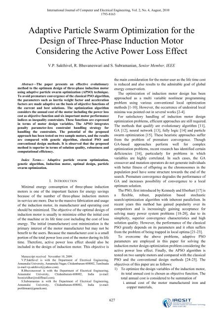
International Journal of Computer and Electrical Engineering, Vol. 2, No. 4, August, 2010
1793-8163
Adaptive Particle Swarm Optimization for the
Design of Three-Phase Induction Motor
Considering the Active Power Loss Effect
V.P. Sakthivel, R. Bhuvaneswari and S. Subramanian, Senior Member, IEEE
Abstract—The paper presents an effective evolutionary
method to the optimum design of three-phase induction motor
using adaptive particle swarm optimization (APSO) technique.
To avoid premature convergence of the classical PSO algorithm,
the parameters such as inertia weight factor and acceleration
factors are made adaptive on the basis of objective functions of
the current and best solutions. The optimization algorithm
considers the annual cost of the motor including the power loss
cost as objective function and six important motor performance
indices as inequality constraints. These functions are expressed
in terms of motor design variables. The APSO integrates
penalty parameter-less constraint handling strategy for
handling the constraints. The potential of the proposed
approach has been tested on two sample motors, and the results
are compared with genetic algorithm, classical PSO and
conventional design methods. It is observed that the proposed
method is superior in terms of solution quality, robustness and
computational efficiency.
Index Terms— Adaptive particle swarm optimization,
genetic algorithm, Induction motor, optimal design, particle
swarm optimization.
I. INTRODUCTION
Minimal energy consumption of three-phase induction
motors is one of the important factors for energy savings
because of the number of three-phase induction motors
in-service are more. Due to the massive fabrication and usage
of the induction motor, its manufacturer and operating cost
should be minimized. The objective of the optimal design of
induction motor is usually to minimize either the initial cost
of the machine or its life time cost including the cost of loss
energy. The initial (manufacturer) cost minimization is the
primary interest of the motor manufacturer but may not be
benefit to the users. Because the manufacturer cost is a small
portion of the total power loss cost of the motor during its life
time. Therefore, active power loss effect should also be
included in the design of induction motor. This objective is
Manuscript received November 10, 2009.
V.P.Sakthivel is with the Department of Electrical Engineering,
Annamalai University, Annamalai Nagar, Chidambaram-608002, Tamilnadu
(e-mail:vp.sakthivel@yahoo.com).
R.Bhuveneswari is with the Department of Electrical Engineering,
Annamalai University, Chidambaram-608002, India (e-mail:
boonisridhar@rediffmail.com).
S.Subramanian is with the Department of Electrical Engineering,
Annamalai University, Chidambaram-608002, India (e-mail:
profdrmani@gmailcom).
627
the main consideration for the motor user as the life time cost
is reduced and also results to the admirable goal of global
energy conservation.
The optimization of induction motor design has been
approached as a multi variable nonlinear programming
problem using various conventional local optimization
methods [1-10]. However, the occurrence of undesired local
minima was pointed out in several works [2-4].
For satisfactory handling of induction motor design
optimization problems, efficient approaches are still required.
The methods that qualify are evolutionary algorithm [11],
GA [12], neural network [13], fully logic [14] and particle
swarm optimization [15]. These heuristic approaches suffer
from the problem of premature convergence. Though
GA-based approaches perform well for complex
optimization problems, recent research has identified certain
deficiencies [16], particularly for problems in which
variables are highly correlated. In such cases, the GA
crossover and mutation operators do not generate individuals
with better fitness of offspring as the chromosomes in the
population pool have some structure towards the end of the
search. Premature convergence degrades the performance of
GA and increases possibility of convergence to a local
optimum solution.
The PSO, first introduced by Kennedy and Eberhart [17] is
a flexible, robust, population based stochastic
search/optimization algorithm with inherent parallelism. In
recent years this method has gained popularity over its
competitors and is increasingly gaining acceptance for
solving many power system problems [18-20], due to its
simplicity, superior convergence characteristics and high
solution quality. However, the performance of the classical
PSO greatly depends on its parameters and it often suffers
from the problem of being trapped in local optima [21-23].
To overcome the above problems, adaptive PSO
parameters are employed in this paper for solving the
induction motor design optimization problem considering the
active power loss effect. Finally, the APSO algorithm is
tested on two sample motors and compared with the classical
PSO and the conventional design methods [24-25]. The
objectives of this paper are as follows:
1) To optimize the design variables of the induction motor,
its total annual cost is chosen as objective function. The
total annual cost is considered to be summation of
i. annual cost of the motor manufactured iron and
copper materials,

International Journal of Computer and Electrical Engineering, Vol. 2, No. 4, August, 2010
1793-8163
ii. annual cost of a fictitious active power source
required to cover the total active power loss of the
motor and
iii. annual cost of energy needed by that fictitious
source.
2) To avoid premature convergence, the inertia weight
factor and the acceleration factors are made adaptive.
3) To handle the constraints effectively, the penalty
parameter-less approach is used.
II. FORMULATION OF AN INDUCTION MOTOR DESIGN
PROBLEM
The problem in the induction motor design is to select an
appropriate combination of the design variables which
minimize the annual cost of the motor. The design problem
would have been much complicated while using too many
variables. Therefore the design variables selection is
important in the motor design optimization. The design has
some constraints to guarantee the some motor performance
indices. The design optimization problem can be formulated
as a general nonlinear programming problem of the standard
form:
Find X(x1, x2, …….., xn) such that J(X) is a minimum
Subject to
gj(X) ≥ 0 j = 1, 2, ……… m
and
xLi ≤ xi ≤ xUi i = 1,2, …………n
where X(x1, x2, …….., xn) is the set of independent design
variables with their lower and upper limits as xLi and xUi, for
all ‘n’ variables. J(X) is the objective function to be
optimized and gj(X) are the constraints imposed on the
design.
A. Variables
The following variables (X1, ….. X9) are considered.
x1 = stator bore diameter
x2 = average air gap flux density
x3 = stator current density
x4 = air gap length
x5 = stator slot depth
x6 = stator slot width
x7 = stator core depth
x8 = rotor slot depth
x9 = rotor slot width
The remaining parameters can be expressed in terms of
these variables or may be treated as fixed for a particular
design.
B. Constraints
The constraints (g1, ….. , g6) imposed into induction motor
design in this paper are as follows.
g1 = maximum to full-load torque ratio
g2 = starting to full-load torque ratio
g3 = starting to full-load current ratio
g4 = full-load efficiency
g5 = full-load power factor
g6 = maximum temperature rise
Apart from these constraints, the lower and upper limits of
the design variables are included. The expression of the
constraint functions is as follows:
(i). Maximum to full-load torque ratio
2
628
⎡⎛
R ⎞
⎢⎜
2
S
⎟
fl
R
⎢⎜
th
+ +
⎟
⎣⎝
S
fl ⎠
=
1 ⎡ 2
2R
2
R + R +
⎢ th th
⎣
(ii). Starting to full-load torque ratio
⎡
2
⎛ R
2 ⎞
S ⎢⎜
fl
R
th
+ ⎟ +
⎢⎜
S ⎟
⎣⎝
fl ⎠
( X
th
(X
th
+
+
2
X )
2
2
X )
2
⎤
⎥
⎥
⎦
⎤
g (1)
g
2
=
( R
th
+
2
R )
2
+
(X
th
( X
th
+
+
2
X )
2
2
X )
2
(iii). Starting to full-load current ratio
g
2
g = (3)
3 S
fl
(iv). Full load power factor
⎡
⎢
⎢
⎢
⎢
⎣
⎛
⎜
⎜
⎜
⎜
⎝
⎞⎤
⎟⎥
⎟⎥
⎟⎥
⎟
⎟⎥
⎠⎦
⎥
⎦
⎤
⎥
⎥
⎦
(2)
−1
X
th
+ X
2
g = cos tan
(4)
4
R
2
R
th
+
S
fl
(v). Full load efficiency
W
g =
5 W + Pt
(5)
Where, P t = P
isc
+ P
ist
+ Psc
+ P
b
+ Per
+ P
f
(vi). Maximum temperature rise
g
6
where, V
th
=
LPsc
P
is
+
L
o
πDo
L πx
1
L π(Do
− x
1
)(2 + n v )
+ +
(6)
Csco
C
sci
4Cscv
=
V
ph
X m
X1
+
X m
,
R
th
=
R1X
m
X1
+
X m
,
X
th
=
X1X
m
X1
+
X m
The equivalent circuit parameters R1, R2, X1, X2 and Xm
can be found in terms of the design variables [24, 25].
C. Objective function
To have an optimal induction motor which is acceptable to
both the manufacturer and the user, the minimization of the
annual cost of the motor is considered as objective function
while designing the motor using optimization algorithms.
The expression of the objective function, in terms of the
motor design variables are as follows:
(i) Annual active material cost
Annual iron material cost,

International Journal of Computer and Electrical Engineering, Vol. 2, No. 4, August, 2010
1793-8163
C
i
= αc
i
( M + M + M + M + M )
isc ist irc irtt irtb
Where,
M
isc
= 0.88π × W
i
K
i
Lx
7
(x + 2x + x )
1 5 7
M
ist
= 0.88π × W
i
K
i
Lx
5
(π ( x + x ) - N x )
1 5 s 6
M
irc
= 0.88π × W
i
K
i
Ld ( D − 2x − d )
rc r 8 rc
M
irtt
= 0.88W
i
K
i
Ldrs
(π ( D − d ) − N x )
r rs r 9
M
irtb
= 0.88W
i
K
i
L ( x - d ) ( π ( D - x - d ) - N x
8 rs r 8 rs r 9
Annual copper material cost,
C c = αcc
( M + M +
sc b
Where,
Msc
M )
er
⎡
⎛ x ⎞ ⎤
= W
⎢ +
⎜ 1
cK
ss x
⎟
5
x
6
Ns
0.0635 0.472 + L⎥
⎣
⎝ p ⎠ ⎦
M
b
= 1.02WcK
sr Lx
9
N r ( x − d )
8 rs
(x
8
− drs
)
Mer
= 1.9WcK
sr x
1
x
9
Nr
K
j
p
Annual active material cost is given by
c C
C m = C
i
+
(9)
(ii) Annual active power loss cost
Annual iron loss cost,
C
ip
= αcp
(P
isc
+ P
ist
)
(10)
Where,
P
isc
= p
isc
M
isc
P
ist
= p
ist
M
ist
Where, pisc and pist are the specific iron loss corresponding
to Bsc and Bst respectively.
Bsc and Bst are given as follows
B sc =
πx
1
x
2
1.76K
i
x
7
p
1.5x x
B =
1 2
st
⎡ 2x
5
0.88K
i ⎢x
1
+ −
⎣ 3
Annual copper loss cost
C cp = αcp
(Psc
+ P
b
+ Per
)
Where,
2
x
3
ρs
Msc
P sc =
Wc
2
δr
ρr
M
b
P
b
=
P er =
Wc
2
(δr
K
j
) ρr
KerM
er
Wc
Ns
x
6
Annual friction and windage loss cost,
C
fp
= αcp
P
f
π
⎤
⎥
⎦
)
(7)
(8)
(11)
(12)
2
3 ⎛ f ⎞
Where, P
f
= 661x
1
L⎜
⎟
⎝ p ⎠
The stray loss is assumed to reduce the efficiency by 0.5%,
so that
C sp = αcp
Ps
(13)
Where,
0.005 × W
Ps
=
η
The total annual active power loss cost is thus
C p = C
ip
+ Ccp
+ C
fp
+ Csp
(14)
629
(iii) Annual energy loss cost
C e =
ce
TCp
αcp
The objective function is given by
J(X) = Cm
+ C + C
p e
III. PARTICLE SWARM OPTIMIZATION
(15)
(16)
PSO is a well known optimization method proposed by
Kennedy and Eberhart [17]. It is motivated by social behavior
of organisms such as fish schooling and bird flocking. In
PSO, potential solutions called particles fly around in a
multi-dimensional problem space. Population of particles is
called swarm. Each particle in a swarm flies in the search
space towards the optimum solution based on its own
experience, experience of nearby particles and global best
position among particles in the swarm.
A. Advantages of PSO
• PSO is easy to implement, and only few parameters have to
be adjusted.
• Unlike the GA, PSO has no evolution operators such as
crossover and mutation.
• In GAs, chromosomes share information so that the whole
population moves like one group, but in PSO, only global
best particle (gbest) gives out information to the others. It
is more robust than GAs.
• PSO can be more efficient than GAs; that is, PSO often
finds the solution with fewer objective function evaluations
than that required by GAs.
• Unlike GAs and other heuristic algorithms, PSO has the
flexibility to control the balance between global and local
exploration of the search space.
B. PSO Algorithm
Let X and V denote the particle’s position and its
corresponding velocity in search space respectively. At
iteration K, each particle i has its position defined by X i K =
[X i, 1, X i, 2 ….X i, N] and a velocity is defined as V i K = [V i, 1,
V i, 2……V i, N] in search space N. Velocity and position of
each particle in the next iteration can be calculated as
V i, n k+1 = W × V i, n k + C1×rand1× (pbest i, n – X i, n k ) +
C2×rand2 ×(gbest n – X i, n k ) (17)
i = 1, 2……… m
n = 1, 2………. N

International Journal of Computer and Electrical Engineering, Vol. 2, No. 4, August, 2010
1793-8163
X i, n k+1 = X i, n k + Vi, n k+1 if Xmin,i, n ≤ X i k+1 ≤ X max i, n (18)
= X min i, n if X i, n k+1 < X min i,n
= X max i, n if Xi, n k+1 > X max i, n
The inertia weight W is an important factor for the PSO’s
convergence. It is used to control the impact of previous
history of velocities on the current velocity. A large inertia
weight factor facilitates global exploration (i.e., searching of
new area) while small weight factor facilitates local
exploration. Therefore, it is wise to choose large weight
factor for initial iterations and gradually reduce weight factor
in successive iterations. This can be done by using
W= W max − (W max – W min) × Iter / Iter max (19)
Acceleration constant C1 called cognitive parameter pulls
each particle towards local best position whereas constant C2
called social parameter pulls the particle towards global best
position. The particle position is modified by Eq. (18). The
process is repeated until stopping criterion is reached.
IV. ADAPTIVE PARTICLE SWARM OPTIMIZATION
In the classical PSO, the inertia weight factor is made
constant for all the particles in a single generation and the
acceleration factors are made constant for all the particles in
the whole generation. But these factors are very important
parameters that move the current position of the particle
towards its optimum position. In order to increase the search
ability, the algorithm should be modified in which the
movement of the swarm should be controlled by the objective
function. In the proposed APSO, the particle position is
adjusted such that the highly fitted particle moves slowly
when compared to the lowly fitted particle. This can be
achieved by using adaptive parameter values for each particle
according to their objective functions of the current and best
solutions.
The adaptive inertia weight factor (AIWF) is obtained as
follows:
k
W
i
k−1
k−1
k−1
J
pbest
× J
i
− J
pbest
W
min
+
k−1
k−1
k−1
J
i
× J
i
− J
best
= (20)
So, from Eq. (19), it can be seen that the inertia weight for
the best particle is set to the minimum value and vice versa.
The adaptive acceleration factors are determined as
follows:
k
C
1, i
k
C
2,i
k−1
J
i
k−1
J
pbest
k−1
J
i
k−1
J
gbest
= (21)
= (22)
It is concluded from Eqs. (20) and (21) that C1 and C2
values are greater than or equal to one. Higher acceleration
factors are obtained for higher objective function and vice
versa. Use of Eqs. (19), (20) and (21) in Eq. (17) is expected
to provide better optimum solution compared to classical
PSO.
630
V. IMPLEMENTATION OF APSO FOR INDUCTION MOTOR
DESIGN PROBLEM
The induction motor design problem with power loss cost
consideration is solved using APSO approach. The PSO
parameters such as inertia weight and acceleration factors are
made highly adaptive to avoid the premature convergence of
the algorithm. Then the parameter-less penalty approach is
incorporated in the proposed algorithm to handle the
constraints effectively.
Fig.1 Computational flowchart of the proposed APSO algorithm
The flow of the APSO is depicted in Fig.1 and is described
as follows:
Step 1. Initialization of the swarm: For a population size m,
the particles are randomly generated between the
minimum and maximum limits of the design
variables.
Defining the fitness function: A suitable fitness function
should be used for constraints handling based on the current
population. In a population, solutions are assigned to fitness
so that feasible solutions are emphasized more than infeasible
solutions. In this paper, a penalty parameter-less approach is
used. This approach uses tournament selection operator
where two solutions are chosen from the population and one
is selected. The following criteria are used during the
selection operator:
• Any feasible solution is preferred to any
infeasible solution.
• Among the two feasible solutions, the one
having better objective value is preferred.
• Among the two infeasible solutions, the one
having smaller constraint violation is preferred.

International Journal of Computer and Electrical Engineering, Vol. 2, No. 4, August, 2010
1793-8163
In this scheme, the objective function value is evaluated
for feasible solutions and not for particles with constraint
violation. The infeasible solutions are compared based on
only their constraint violation values. Motivated by this
argument, the following composite fitness function is used.
J(X) = J(X) if x is feasible
J max + CV(X) otherwise
(23)
Where, J max is the objective function of the worst feasible
solution in the population. CV(X) is the overall constraint
violation of solution X. It is calculated as follows:
CV(X) = max (0, g1(s) – g1(c)) + max (0, g2(s) –
g2(c)) + max (0, g3(c) – g3(s)) + max (0,
g4(s) – g4(c)) + max (0, g5(s)-g5(c)) + max
(0, g6(c) – g6(s)) (24)
where c and s denote the computed and specified
constraint values respectively.
Step 2. Initialization of pbest and gbest: The fitness values
obtained above for the initial particles of the swarm
are set as the initial pbest values of the particles. The
best value among all the pbest values is identified as
gbest.
Step 3. Evaluation of adaptive inertia weight and
acceleration factors: The inertia weight and
acceleration factors are computed using Eqs. (20),
(21) and (22).
Step 4. Evaluation of velocity: The new velocity for each
particle is computed as
V i, n k+1 =
k
W i × V i, n k +
k
2 i
k
1 i
C ×rand1× (pbest i, n –
X i, n k ) + C ×rand2 ×(gbest n – X i, n k ) (25)
Step 5. Update the swarm: The particle position is updated
using Eq. (18). The values of the fitness function are
calculated for the updated positions of the particles.
If the new value is better than the previous pbest, the
new value is set to pbest. Similarly, gbest value is
also updated as the best pbest.
Step 6. Stopping criteria: A stochastic optimization
algorithm is usually stopped either based on the
tolerance limit or when maximum number of
generations are reached. The number of generations
is used as the stopping criterion in this paper.
VI. RESULTS AND DISCUSSIONS
In order to verify the efficiency and effectiveness of the
proposed APSO, two sample motors are used, whose
specifications are given in Appendix B. The results obtained
by this method are compared with the GA, classical PSO and
conventional design methods [24, 25]. The value of design
constants is given in Appendix C.
A. Parameter selection
For PSO method, a population size (m) of 10 is selected,
the maximum number of iteration is set to 50, the acceleration
constants C1 and C2 are both set to 2.0, and the inertia weight
(W) is varied linearly from 0.9 to 0.3 over 50 iterations. In
the proposed APSO approach, the population size and the
maximum number of iteration are the same as those used in
PSO approach, and the inertia weight and acceleration factors
631
are made adaptive using Eqs. (20), (21), and (22).
Fig. 2 Variations of W with iterations for motor 1
Fig. 3 Variations of C1 with iterations for motor 1
Fig. 4 Variations of C2 with iterations for motor 1

International Journal of Computer and Electrical Engineering, Vol. 2, No. 4, August, 2010
1793-8163
TABLE I: INDIVIDUAL ANNUAL COMPONENTS OF MOTOR 1
Annual cost components Conventional
Case 1 Case 2
approach GA PSO APSO GA PSO APSO
Material
Iron (Rs) 142.33 141.37 147.16 139.33 166.84 163.12 166.53
Copper (Rs) 344.77 319.05 352.27 299.6 397.35 353.9 319.34
Total (Rs)
Power loss
487.1 460.42 499.43 438.9 564.19 517.02 485.87
Iron (Rs) 339.27 317.87 328.04 311.6 351.12 344.29 338.07
Copper (Rs) 566.08 522.15 487.91 494.04 422.57 427.53 420.54
Friction and windage (Rs) 43.66 40.82 42.78 42.22 43.29 42.3 41.08
Stray (Rs) 32.01 31.72 31.28 32.28 30.3 30.44 30.54
Total (Rs)
Energy loss
981.02 912.56 890.01 880.14 847.28 844.56 830.23
Iron (Rs) 1769 1657.5 1710.5 1624.7 1830.8 1795.2 1762.8
Copper (Rs) 2951.7 2722.6 2544.1 2576 2203.4 2229.3 2192.8
Friction and windage (Rs) 227.65 212.83 223.12 220.15 225.75 220.57 214.2
Stray (Rs) 166.89 165.37 163.10 168.34 158.04 158.72 159.22
Total (Rs) 5115.24 4758.3 4640.8 4589.19 4418 4403.79 4329.02
Total annual cost (Rs) 6583.36 6131.28 6030.2 5908.23 5829.5 5765.37 5645.12
TABLE II: OPTIMUM DESIGN RESULTS OF MOTOR 1 FOR DIFFERENT APPROACHES
Variables/ indices Conventional
Case 1 Case 2
approach GA PSO APSO GA PSO APSO
Independent variables
Stator bore diameter (mm) 150 145 145.7 146 138 137 135
Average air gap flux density (Wb/m 2 ) 0.46 0.476 0.456 0.463 0.427 0.435 0.44
Stator current density (A/mm 2 ) 4 4.2 4.02 4.7 3.54 3.65 3.9
Air gap length (mm) 0.43 0.41 0.39 0.46 0.35 0.33 0.302
Stator slot depth (mm) 24.15 22.8 22.74 21.55 28 27.8 26.38
Stator slot width (mm) 6.92 7.2 7.15 7.13 7.6 7.8 7.84
Stator core depth (mm) 24.94 26.6 26.4 26.32 29.5 29.7 30.8
Rotor slot depth (mm) 10 10 12 8.8 13.6 11 13.2
Rotor slot width (mm)
Dependent Variables
5 4.6 5 5 6 6 4
Gross iron length (mm) 89 92.6 95.8 93.8 11.4 112.7 115.5
Rotor current density (A/mm 2 )
Performance index
7.74 7.6 7.4 7.24 6.1 6.4 5.9
Maximum to full-load torque ratio 2.21 2.57 2.7 2.64 3.3 2.6 2.2
Starting to full-load torque ratio 1.27 1.6 1.37 1.48 1.23 1.15 1.15
Starting to full-load current ratio 4.15 4.92 4.68 4.8 4.1 4.2 3.8
Full-load efficiency 81.57 82.32 83.47 81.8 86.15 85.77 85.71
Full-load power factor 0.86 0.82 0.84 0.87 0.88 0.89 0.89
Maximum temperature rise 52 50.68 49.68 51.87 46.6 46.7 46.74
TABLE III: INDIVIDUAL ANNUAL COMPONENTS OF MOTOR 2
Annual cost components Conventional
Case 1 Case 2
approach GA PSO APSO GA PSO APSO
Material
Iron (Rs) 246.87 238.5 237.4 236.9 253.04 245.3 257.44
Copper (Rs) 568.32 514.0 519.8 507.3 687.15 575.61 718.38
Total (Rs)
Power loss
815.19 752.5 757.2 744.2 940.19 820.91 975.82
Iron (Rs) 633.16 631.48 611.1 607.8 624.99 610.42 591.51
Copper (Rs) 752.79 745.63 767.41 759.78 702.2 732.23 719.42
Friction and windage (Rs) 86.51 86.1 83.03 82.55 73.69 73.08 70.565
Stray (Rs) 61.09 61.11 61.37 61.08 60.5 60.98 60.26
Total (Rs)
Energy loss
1533.55 1524.32 1523 1511.21 1461.4 1476.7 1441.75
Iron (Rs) 3301.5 3292.8 3186.4 3169.2 3258.9 3182.9 3084.3
Copper (Rs) 3925.3 3887.9 4001.5 3962.3 3661.5 3818 3751.3
Friction and windage (Rs) 451.08 448.98 432.95 430.44 384.27 381 367.95
Stray (Rs) 318.59 318.65 320 318.5 315.5 318 314.24
Total (Rs) 7996.47 7948.33 7940 7880.44 7620.2 7700 7517.79
Total annual cost (Rs) 10345.21 10225.1 10220 10135.85 10022 9997.6 9935.36
632

International Journal of Computer and Electrical Engineering, Vol. 2, No. 4, August, 2010
1793-8163
TABLE IV: OPTIMUM DESIGN RESULTS OF MOTOR 2 FOR DIFFERENT APPROACHES
Variables/ indices Conventional
Case 1 Case 2
approach GA PSO APSO GA PSO APSO
Independent variables
Stator bore diameter (mm) 165 163 164 162 139 136 131.6
Average air gap flux density (Wb/m 2 ) 0.45 0.465 0.466 0.463 0.445 0.45 0.44
Stator current density (A/mm 2 ) 4 4.04 4.17 4.05 3.9 4.02 3.81
Air gap length (mm) 0.35 0.388 0.38 0.384 0.33 0.37 0.33
Stator slot depth (mm) 25 26.84 26.9 26.5 27.88 27.3 24.5
Stator slot width (mm) 7 7.5 7.4 7.3 6.5 6.6 6.3
Stator core depth (mm) 26 27.5 26.7 26.2 27.89 22 27.5
Rotor slot depth (mm) 13 13 10 10 14 12.8 14
Rotor slot width (mm)
Dependent Variables
4 3.8 5 4.65 5 6.8 5
Gross iron length (mm) 133.2 122 130.2 134 189.8 186.6 214.1
Rotor current density (A/mm 2 )
Performance index
5.13 6.07 6.36 6.28 4.6 4.84 4.08
Maximum to full-load torque ratio 2.5 2.8 2.73 2.43 3.04 2.06 2.52
Starting to full-load torque ratio 0.975 1.25 1.28 1.1 1.01 1.02 0.88
Starting to full-load current ratio 3.6 4.8 4.92 3.89 4.6 4.7 3.11
Full-load efficiency 85.5 85.45 85.08 85.65 86.3 85.62 86.65
Full-load power factor 0.9 0.92 0.92 0.917 0.92 0.91 0.92
Maximum temperature rise 60 61.2 60.08 58.72 55.53 56 51.38
TABLE V: COMPARISON OF DIFFERENT METHODS FOR MOTOR 1 (20-TRIALS)
Compared item Case 1 Case 2
GA PSO APSO GA PSO APSO
Maximum cost (Rs) 6423.63 6217.36 6055.12 6116.2 5940.29 5779.77
Minimum cost (Rs) 6131.28 6030.2 5908.23 5829.5 5765.37 5645.12
Mean cost (Rs) 6293.2 6134.8 6001.2 5949.8 5803.1 5653.4
Standard deviation of cost (Rs) 81.2 61.61 46.52 86.8 65.45 42.6
TABLE VI: COMPARISON OF DIFFERENT METHODS FOR MOTOR 2 (20-TRIALS)
Compared item Case 1 Case 2
GA PSO APSO GA PSO APSO
Maximum cost (Rs) 10499.46 10413.23 10260.74 10299.65 10161.12 10054.59
Minimum cost (Rs) 10225 10220 10135.85 10022 9997.6 9935.36
Mean cost (Rs) 10338 10319 10213 10154 10060 9999.4
Standard deviation of cost (Rs) 87.67 55.76 40.05 84.23 50.6 36.16
TABLE VII : COMPARISON OF COMPUTATION TIME (IN SECONDS) OF
VARIOUS METHODS
Methods Motor 1 Motor 2
Case 1 Case 2 Case 1 Case 2
GA 3.2 3.3 3.42 3.5
PSO 2.72 2.88 2.68 2.87
APSO 3.05 3.13 3.28 3.37
The variation of inertia weight and acceleration factors
with the number of iterations for the sample motor 1 has been
shown in Figs. 2, 3 and 4. From the figures it is obvious that,
W varies between 1 and 0.3, and the C1 and C2 values are
large at the starting and it reaches unity as the problem
converges.
B. Case study
To demonstrate the effectiveness of the proposed approach,
two cases have been considered as follows:
Case 1: The annual active material cost is considered as
objective.
Case 2: The total annual cost of the motor is considered as
objective.
The optimal annual cost and its individual components of
633
the sample motors obtained from the various approaches are
given in Tables I and III. Tables II and IV give the value of
design variables and their performance indices of APSO
approach in comparison with those of GA, PSO and
conventional approaches.
From the obtained results of Tables I and III, it is obvious
that the annual cost of the motors is considerably reduced
when designed on the basis of Case 2; instead of Case 1and
the proposed approach provides lower annual cost than the
other aforementioned approaches. In Case 2 based design of
induction motors, the values of air gap density and stator
current density are lower than those of Case 1 based design.
These design variables are inversely proportional to the
active material cost and the efficiency of the motor, and
therefore the active material cost and the efficiency of the
motor for Case 2 are higher than the Case 1. The increased
active material cost for Case 2 is negligible when compared
with the decreased motor loss cost. Due to reduction in the air
gap flux density and air gap length of the design, the full load
power factor is improved in Case 2. The starting current for
Case 2 is lower than that of Case 1, because of the increase in
leakage reactance due to decrease in the value of the air gap
length. The maximum torque and the starting torque to full

International Journal of Computer and Electrical Engineering, Vol. 2, No. 4, August, 2010
1793-8163
load ratios of Case 2 are adversely affected. However, their
values remain within the permissible given limits.
Fig. 5 Convergence Characteristic of different approaches for motor 1
Fig. 6 Convergence Characteristic of different approaches for motor 2
C. Comparison with GA and PSO approaches
(i) Convergence behaviors
The convergence behaviors for the GA, PSO and APSO
approaches of the two sample motors are shown in Figs. 5
and 6. It is observed that, the GA and PSO approaches
saturate quickly and converge to a local optimum solution.
But the APSO approach shows superior performance because
the premature convergence is avoided by using the adaptive
parameters.
(ii) Solution quality
The minimum, maximum, average and standard deviation
costs obtained from 20 trials for GA, PSO and APSO are
given in Tables V and VI. It can be seen that the proposed
method yields smaller standard deviation of costs and lower
annual cost than the other approaches.
(iii) Robustness
To verify the robustness/consistency of three different
approaches, many trials with different initial populations are
634
carried out. The lowest cost for each of the 20 different trials
has been plotted in Figs. 7 and 8 from which it can be found
Fig. 7 Best results of different approaches for motor 1
Fig. 8 Best results of different approaches for motor 2
that APSO approach produces lowest annual cost of the
motor most consistently as compared to the GA and PSO.
(iv) Computation efficiency
The comparison of computation efficiency for various
approaches is given in Table VII. From Table VII, it is clear
that the average CPU time of the APSO approach is lesser
than those of the GA, but it is more than the PSO method.
This is due to the introduction of adaptive parameters in
every evolutionary process.
VII. CONCLUSION
The adaptive particle swarm optimization (APSO)
approach has been proposed for solving the complex
induction motor design problem considering the active power
loss effect. In this approach, the parameters such as inertia
weight and acceleration factors are made adaptive to avoid
the premature convergence of the algorithm. The constraints
are handled by a penalty-parameter-less penalty approach. In
order to verify the efficiency and effectiveness of the

International Journal of Computer and Electrical Engineering, Vol. 2, No. 4, August, 2010
1793-8163
proposed APSO approach, two sample motors are
investigated. The performance of this approach is compared
with the GA, classical PSO and conventional design
approaches, and it is found that APSO outperforms the other
approaches in terms of solution quality, convergence and
robustness. Hence, the APSO approach is an efficient tool for
finding optimized values of design variables of the induction
motor. Further work is in progress to develop the actual
motor setup.
APPENDIX A.
LIST OF SYMBOLS
Ci annual iron material cost (Rs)
Cip annual iron loss cost (Rs)
Ccp annual copper loss cost (Rs)
Cfp annual friction and windage losses cost (Rs)
Csp annual stray loss cost (Rs)
Cc annual copper material cost (Rs)
Cp annual active power loss cost (Rs)
Ce annual energy loss cost (Rs)
Cm annual active material cost (Rs)
Misc, Mist core and tooth iron masses in stator (Kg)
Mirc, Mirtb, Mirtt core, tooth bodies and tooth tips iron
masses in rotor (Kg)
Mb, Mer, Msc bars, end rings and stator conductor copper
masses (Kg)
pisc, pist specific iron loss of stator core and tooth (W/Kg)
Pisc, Pist core and teeth iron power loss in stator (W)
Pb, Per, Psc bars, end rings and stator conductors copper
power
losses (W)
Pf, Ps
friction and stray power losses (W)
Ksr, Kss rotor and stator slot copper insulating factors
δr rotor current densities (A/mm 2 )
P number of poles
T motor running time per year (hr)
α annual rate of interest and depreciation
ηfl full-load efficiency
W rated power (W)
Ker end ring non-uniformity current distribution
factor
Wc, Wi copper and iron specific masses (Kg/m 3 )
ρs, ρr stator and rotor copper resistivities (Ω.m)
Bsc, Bst Flux density of stator core and teeth (Tesla)
Ki iron insulation factor
Kj end ring to bar current density ratio
f supply frequency (Hz)
Vph Voltage per phase (V)
Nr, Ns
rotor and stator number of slots
cc, ci specific copper and iron material costs (Rs/Kg)
ce specific energy loss cost (Rs/Wh)
cp specific power loss cost (Rs/W)
drc rotor core depth (m)
drs rotor slot opening depth (m)
wrs rotor slot opening width (m)
Di rotor inner diameter (m)
635
Do stator outer diameter (m)
Dr rotor diameter (m)
L gross iron length (m)
Li active iron length (m)
Lo Length of the conductor overhang (m)
R1, R2
resistances of stator and rotor (Ω)
X1, X2, Xm stator, rotor and magnetizing reactances (Ω)
Vth, Rth, Xth Thevenin’s equivalent voltage, resistance and
reactance
Sfl full-load slip
Smax Slip at which maximum torque occurs
Csco, Csci, Cscv cooling coefficients for stator core outer,
inner and ventilating ducts
m number of particles in the swarm
N number of dimensions in a particle
K pointer of iterations (generations)
Vi, n k velocity of particle i at iteration k
W weighting factor
C j acceleration factor
rand j
random number between 0 and 1
X i, n k current position of particle i at iteration k
pbest i personal best of particle i
gbest global best of the group
W max final weight
W min initial weight
Iter current iteration number
maximum iteration number
Iter max
k
W
i inertia weight of ith population at kth iteration
k 1
J
i
− objective value of ith solution at (K-1)th iteration
k 1
J
pbest
−
objective value of pbest solution at (K-1)th
k 1
J
gbest
−
k k
1,i
, C
2,i
iteration
objective value of gbest solution upto (K-1)th
iteration
C first and second acceleration factors for the ith
population at kth iteration respectively
APPENDIX B
SPECIFICATION OF TEST MOTORS
Sample motor 1
Capacity 5 HP
Voltage 400V
Current 7.8A
Frequency 50 Hz
No. of Poles 4
Full load power factor 0.8
Full load efficiency 83%
Sample motor 2
Capacity 10 HP
Voltage 415V
Current 13.68A
Frequency 50Hz

No. of Poles 4
Full load power factor 0.87
Full load efficiency 87%
International Journal of Computer and Electrical Engineering, Vol. 2, No. 4, August, 2010
1793-8163
APPENDIX C
ASSUMED DESIGN CONSTANTS
α = 0.2, Wi = 7600Kg/m 3 , Wc = 8900 Kg/m 3 , ci = 35 Rs/Kg,
cc = 250 Rs/Kg, ce = 0.002 Rs/Wh, cp = 7 Rs/W, ρr = 2.1 ×
10 -8 , ρs = 2.51 × 10 -8 , Ki = 0.9, Kj = 1; T = 3650 hr, Ns = 36, Nr
= 30.
REFERENCES
[1] O.W. Anderson, “Optimum design of electrical machines,” IEEE Trans.
on Power Apparatus and Systems, vol. 86, 1967, pp. 707-711.
[2] R. Ramarathnam, and B.G. Desai, “Optimization of poly-phase
induction motor design – a nonlinear programming approach,” IEEE
Trans. Power Apparatus and Systems, vol. 90, 1971, pp. 570-578.
[3] C. Li, and A. Rahman, “Three-phase induction motor design
optimization using the modified Hooke-Jeeves method,” Electrical
Machines and Power Systems, vol. 18, 1990, pp. 1-12
[4] R. Ramarathnam, B.G. Desai, and V. Subba Rao, “A comparative study
of minimization techniques for optimization of induction motor
design,” IEEE Trans. Power Apparatus and Systems, vol. 92, 1973, pp.
1448-1454.
[5] M. Nurdin, M. Poloujadoff, and A. Faure, “Synthesis of squirrel cage
motors: A key to optimization,” IEEE Trans. Energy Convers., vol. 6,
no. 2, 1991, pp. 327-335.
[6] B. Singh, B.P. Singh, S.S. Murthy, and C.S. Jha, “Experience in design
optimization of induction motor using “SUMT” algorithm,” IEEE
Trans. Power Apparatus and Systems, vol. 102, no. 10, 1984, pp.
3379-3384.
[7] N.H. Feith, and H.M. EI-Shewy, “Induction motor optimum design
including active power loss effect,” IEEE Trans. Energy Convers., vol.
1, no. 3, 1986, pp. 155-160.
[8] B.G. Bharadwal, K. Venkatesen, and R. B. Saxena, “Experience with
direct and indirect search methods applied to cage induction motor
design optimization,” Electric Machines and Electromechanics, vol.4,
no. 1, 1979, pp. 85-93.
[9] J. Appelbaum, E.F. Fuchs, and J. C. White, “Optimization of
three-phase induction motor, part I: Formation of the optimization
technique,” IEEE Trans. Energy Convers., vol.2, no. 3, 1987, pp.
407-415.
[10] J. Appelbaum, I.A. Khan, E. F. Fuchs, and J.C. White, “Optimization of
three-phase induction motor, part II: the efficiency and cost of an
optimum design,” IEEE Trans. Energy Convers., vol. 2, no. 3, 1987, pp.
415-422.
[11] Jan Pawel Wieczorek, Ozdemir Gol, and Zbigniew Michalewiez, “An
evolutionary algorithm for the optimal design of induction motors,”
IEEE Trans. Magnetics, vol. 34, no. 6, 1998, pp. 3882-3887.
[12] G. Fuat Uler, Osama A. Mohammed, and Chang-Seop Koh, “Design
optimization of electrical machines using genetic algorithms,” IEEE.
Trans. Magnetics, vol. 31, no. 3, 1995, pp. 2008-2011.
[13] G.T. Bellarmine, R. Bhuvaneswari, and S. Subramanian, “Radial basis
function network based design optimization of induction motor,”
Proceedings of IEEE SOUTHEASTCON 2006, Memphis,
Tennessee, USA, 2006, pp. 75-80.
[14] R. Bhuvaneswari, and S. Subramanian, “Fuzzy logic approach to
three-phase induction motor design,” Proceedings of the International
Conference on Computer Applications in Electrical Engineering
Recent Advances - CERA-05, IIT, Roorkee, India, 2005, Sept 28-Oct 1,
pp. 505-509.
[15] S. Subramanian, and R. Bhuvaneswari, “Optimal design of
single-phase induction motor using particle swarm optimization,”
International Journal of Computation and Mathematics in Electrical
and Electronics Engineering- COMPEL, vol. 26, no. 2, 2007, pp.
418-430.
[16] D.B. Fogel, “Evolutionary Computation: Toward a new philosophy of
machine intelligence,” 2 nd edition, Piscataway, NJ: IEEE Press., 2000
636
[17] J. Kennedy, and R. Eberhart, “Particle Swarm Optimization,”
Proceedings of the IEEE conference on neural networks – ICNN’95,
vol. IV, Perth, Australia, 1995, pp. 1942-1948.
[18] A.A. EL-Dib, H.K.M. Youssef, M.M. EL-Metwally, and Z. Osman,
“Maximum loadability of power system using hybrid particle swarm
optimization,” Electric Power System Research, 2006, no. 76, pp.
485-492.
[19] Y. Ma, C. Jiang, Z. Hou, and C. Wang, “The formulation of the optimal
strategies for the electricity producers based on the particle swarm
optimization,” IEEE Trans. Power Syst., vol. 21, no. 4, 2006, pp.
1663-1671.
[20] J.G. Vlachogiannis, and K.Y. Lee, “A comparative study on particle
swarm optimization for optimal steady state performance of power
systems,” IEEE Trans. Power Syst., vol. 21, no. 4, 2006, pp.
1718-1727.
[21] Y. Shi, and R.C. Eberhart, “Empirical study of particle swarm
optimization,” Proceedings of the IEEE International Congress
Evolutionary Computation, no. 3, 1999, pp. 101-106.
[22] R.C. Eberhart, and Y. Shi, “Comparing inertia weights and constriction
factors in particle swarm optimization,” Proceedings of the IEEE
International Congress Evolutionary Computation, no. 1, 2000, pp.
84-88.
[23] A. Ratnaweera, S.K. Halgamuge, and H.C. Watson, “Self-organizing
hierarchical particle swarm optimizer with time varying acceleration
coefficients,” IEEE Trans. Evol. Comput., vol. 8, no. 3, 2004, pp.
240-255.
[24] M.G. Say, “Alternating Current Machines,” Pitman, 1983.
[25] R.K. Agarwal, “Electrical Machine Design,” 3 rd edition, S.K. Katarai
and Sons, Delhi, 1997
V.P. Sakthivel is Lecturer in Electrical Engineering, Annamalai University,
India. He received the B.E. (Electrical) and M.E. (Power Systems) degrees
from Madras University and Annamalai University, in 2001 and 2004,
respectively. He is currently working towards the Ph.D. degree at Annamalai
University.
His research interests are design and analysis of electrical machines and
optimization techniques applied to machine design.
R. Bhuvaneswari is a Reader in the Department of Electrical Engineering,
Annamalai University, India. She received the B.E. (Electrical), M.E.
(Power Systems) and Ph.D. degrees in the year 1992, 2002 and 2007
respectively from Annamalai University. She has guided 8 BE projects, and
8 ME projects. She has published 25 research papers in various refereed
national and international journals and conferences. She is a review
committee member for various Journals.
Her areas of interest include power system operation and control, design
analysis of electrical machines, power system state estimation and power
system voltage stability studies.
S. Subramanian is Professor of Electrical Engineering, Annamalai
University, India. He received the Ph.D. degree in the area of Power System
Economics in the year 2001 from Annamalai University. He has guided 20
BE projects, 25 ME projects and 5 PhD projects. He is now guiding 8
students towards Ph.D. programme. He visited Singapore and Malaysia for
technical paper presentation. He has published 105 research papers in
various refereed national and international journals and conferences. He is a
senior member of the IEEE, Fellow of the Institution of Engineers (India),
Member of the System Society of India, Indian Society for Technical
Education and of the Indian Science Congress Association.
His areas of research interest include power system operation and control,
design analysis of electrical machines, power system state estimation and
power system voltage stability studies. He received the best teacher award
from Annamalai University in the year 2009.