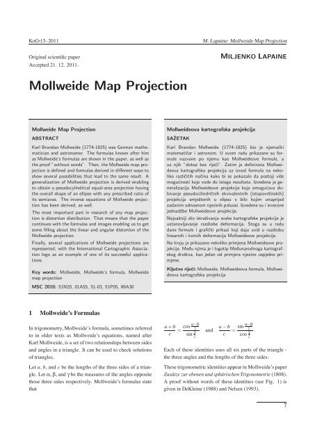
Mollweide Map Projection
Mollweide Map Projection
Mollweide Map Projection

You also want an ePaper? Increase the reach of your titles
YUMPU automatically turns print PDFs into web optimized ePapers that Google loves.
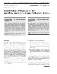
KoG •15–2011 M. Lapaine: <strong>Mollweide</strong> <strong>Map</strong> <strong>Projection</strong><br />
Original scientific paper<br />
Accepted 21. 12. 2011.<br />
<strong>Mollweide</strong> <strong>Map</strong> <strong>Projection</strong><br />
<strong>Mollweide</strong> <strong>Map</strong> <strong>Projection</strong><br />
ABSTRACT<br />
Karl Brandan <strong>Mollweide</strong> (1774-1825) was German mathematician<br />
and astronomer. The formulas known after him<br />
as <strong>Mollweide</strong>’s formulas are shown in the paper, as well as<br />
the proof ”without words”. Then, the <strong>Mollweide</strong> map projection<br />
is defined and formulas derived in different ways to<br />
show several possibilities that lead to the same result. A<br />
generalization of <strong>Mollweide</strong> projection is derived enabling<br />
to obtain a pseudocylindrical equal-area projection having<br />
the overall shape of an ellipse with any prescribed ratio of<br />
its semiaxes. The inverse equations of <strong>Mollweide</strong> projection<br />
has been derived, as well.<br />
The most important part in research of any map projection<br />
is distortion distribution. That means that the paper<br />
continues with the formulas and images enabling us to get<br />
some filling about the linear and angular distortion of the<br />
<strong>Mollweide</strong> projection.<br />
Finally, several applications of <strong>Mollweide</strong> projections are<br />
represented, with the International Cartographic Association<br />
logo as an example of one of its successful applications.<br />
Key words: <strong>Mollweide</strong>, <strong>Mollweide</strong>’s formula, <strong>Mollweide</strong><br />
map projection<br />
MSC 2010: 51N20, 01A55, 51-03, 51P05, 86A30<br />
1 <strong>Mollweide</strong>’s Formulas<br />
In trigonometry, <strong>Mollweide</strong>’s formula, sometimes referred<br />
to in older texts as <strong>Mollweide</strong>’s equations, named after<br />
Karl <strong>Mollweide</strong>, is a set of two relationships between sides<br />
and angles in a triangle. It can be used to check solutions<br />
of triangles.<br />
Let a, b, and c be the lengths of the three sides of a triangle.<br />
Let α, β, and γ be the measures of the angles opposite<br />
those three sides respectively. <strong>Mollweide</strong>’s formulas state<br />
that<br />
MILJENKO LAPAINE<br />
<strong>Mollweide</strong>ova kartografska projekcija<br />
SAˇZETAK<br />
Karl Brandan <strong>Mollweide</strong> (1774-1825) bio je njemački<br />
matematičar i astronom. U ovom radu prikazane su formule<br />
nazvane po njemu kao <strong>Mollweide</strong>ove formule, a<br />
uz njih ”dokaz bez riječi”. Zatim je definirana <strong>Mollweide</strong>ova<br />
kartografska projekcija uz izvod formula na nekoliko<br />
različitih načina kako bi se pokazalo da postoji viˇse<br />
mogućnosti koje vode do istoga rezultata. Izvedena je generalizacija<br />
<strong>Mollweide</strong>ove projekcije koja omogućava dobivanje<br />
pseudocilindričnih ekvivalentnih (istopovrˇsinskih)<br />
projekcija smjeˇstenih u elipsu s bilo kojim unaprijed<br />
zadanim odnosnom njezinih poluosi. Izvedene su i inverzne<br />
jednadˇzbe <strong>Mollweide</strong>ove projekcije.<br />
Najvaˇzniji dio istraˇzivanja svake kartografske projekcije je<br />
ustanovljavanje razdiobe deformacija. Stoga su u radu<br />
dane formule i grafički prikazi koji daju uvid u razdiobu<br />
linearnih i kutnih deformacija <strong>Mollweide</strong>ove projekcije.<br />
Na kraju je prikazano nekoliko primjena <strong>Mollweide</strong>ove projekcije.<br />
Med- u njima je i logotip Med- unarodnoga kartografskog<br />
druˇstva, kao jedan od primjera njezine uspjeˇsne primjene.<br />
Ključne riječi: <strong>Mollweide</strong>, <strong>Mollweide</strong>ova formula, <strong>Mollweide</strong>ova<br />
kartografska projekcija<br />
a + b<br />
c<br />
α−β<br />
cos 2 =<br />
sin γ<br />
2<br />
and<br />
a − b<br />
c<br />
α−β<br />
sin 2 =<br />
cos γ .<br />
2<br />
Each of these identities uses all six parts of the triangle -<br />
the three angles and the lengths of the three sides.<br />
These trigonometric identities appear in <strong>Mollweide</strong>’s paper<br />
Zusätze zur ebenen und sphärischen Trigonometrie (1808).<br />
A proof without words of these identities (see Fig. 1) is<br />
given in DeKleine (1988) and Nelsen (1993).<br />
7
KoG •15–2011 M. Lapaine: <strong>Mollweide</strong> <strong>Map</strong> <strong>Projection</strong><br />
Figure 1: <strong>Mollweide</strong> equation - Proof without Words.<br />
According DeKleine (1988).<br />
One of the more puzzling aspects is why these equations<br />
should have become known as the <strong>Mollweide</strong> equations<br />
since in the 1808 paper in which they appear <strong>Mollweide</strong><br />
refers the book by Antonio Cagnoli (1743-1816) Traité<br />
de Trigonométrie Rectiligne et Sphérique, Contenant des<br />
Méthodes et des Formules Nouvelles, avec des Applications<br />
à la Plupart des Problêmes de l’astronomie (1786)<br />
which contains the formulas. However, the formulas go<br />
back to Isaac Newton, or even earlier, but there is no doubt<br />
that <strong>Mollweide</strong>’s discovery was made independently of<br />
this earlier work (URL1).<br />
2 <strong>Mollweide</strong> <strong>Map</strong> <strong>Projection</strong> Equations<br />
Pseudocylindrical map projections have in common<br />
straight parallel lines of latitude and curved meridians. Until<br />
the 19th century the only pseudocylindrical projection<br />
with important properties was the sinusoidal or Sanson-<br />
Flamsteed. The sinusoidal has equally spaced parallels<br />
of latitude, true scale along parallels, and equivalency or<br />
equal-area. As a world map, it has disadvantage of high<br />
distortion at latitudes near the poles, especially those farthest<br />
from the central meridian (Fig. 2).<br />
Figure 2: Sanson or Sanson-Flamsteed or Sinusoidal projection<br />
In 1805, <strong>Mollweide</strong> announced an equal-area world map<br />
projection that is aesthetically more pleasing than the sinusoidal<br />
because the world is placed in an ellipse with<br />
axes in a 2:1 ratio and all the meridians are equally spaced<br />
8<br />
semiellipses. The <strong>Mollweide</strong> projection was the only new<br />
pseudocylindrical projection of the nineteenth century to<br />
receive much more than academic interest (Fig. 3).<br />
Figure 3: <strong>Mollweide</strong> projection<br />
<strong>Mollweide</strong> presented his projection in response to a new<br />
globular projection of a hemisphere, described by Georg<br />
Gottlieb Schmidt (1768-1837) in 1803 and having the<br />
same arrangement of equidistant semiellipses for meridians.<br />
But Schmidt’s curved parallels do not provide<br />
the equal-area property that <strong>Mollweide</strong> obtained (Snyder,<br />
1993).<br />
O’Connor and Robertson (URL1) stated that <strong>Mollweide</strong><br />
produced the map projection to correct the distortions in<br />
the Mercator projection, first used by Gerardus Mercator<br />
in 1569. While the Mercator projection is well adapted for<br />
sea charts, its very great exaggeration of land areas in high<br />
latitudes makes it unsuitable for most other purposes. In<br />
the Mercator projection the angles of intersection between<br />
the parallels and meridians, and the general configuration<br />
of the land, are preserved but as a consequence areas and<br />
distances are increasingly exaggerated as one moves away<br />
from the equator. To correct these defects, <strong>Mollweide</strong> drew<br />
his elliptical projection; but in preserving the correct relation<br />
between the areas he was compelled to sacrifice configuration<br />
and angular measurement. The <strong>Mollweide</strong> projection<br />
lay relatively dormant until J. Babinet reintroduced<br />
it in 1857 under the name homalographic. The projection<br />
has been also called the Babinet, homalographic, homolographic<br />
and elliptical projection. It is discussed in many<br />
articles, see for example Boggs (1929), Close (1929), Feeman<br />
(2000), Philbrick (1953), Reeves (1904) and Snyder<br />
(1977) and books or textbooks by Fiala (1957), Graur<br />
(1956), Kavrajskij (1960), Kuntz (1990), Maling (1980),<br />
Snyder (1987, 1993), Solov’ev (1946) and Wagner (1949).<br />
The well known equations of the <strong>Mollweide</strong> projections<br />
read as follows:<br />
x = √ 2Rsinβ (1)<br />
y = 2√2 Rλcosβ<br />
π<br />
(2)<br />
2β + sin2β = πsinϕ. (3)
KoG •15–2011 M. Lapaine: <strong>Mollweide</strong> <strong>Map</strong> <strong>Projection</strong><br />
In these formulas x and y are rectangular coordinates in<br />
the plane of projection, ϕ and λ are geographic coordinates<br />
of the points on the sphere and R is the radius of<br />
the sphere to be mapped. The angle β is an auxiliary angle<br />
that is connected with the latitude ϕ by the relation (3).<br />
For given latitude ϕ, the equation (3) is a transcendental<br />
equation in β. In the past, it was solving by using tables<br />
and interpolation method. In our days, it is usually solved<br />
by using some iterative numerical method, like bisection<br />
or Newton-Raphson method.<br />
2.1 First approach<br />
A half of the sphere with the radius R should be mapped<br />
onto the disk with the radius ρ (adopted from Borčić,<br />
1955). If we request that the area of the hemisphere is<br />
equal to the area of the disk, than there is the following<br />
relation:<br />
2R 2 π = ρ 2 π (4)<br />
from where we have<br />
ρ = √ 2R. (5)<br />
Let the circle having the radius ρ be the image of the meridians<br />
with the longitudes λ = ± π 2 . From Fig. 4 we see that<br />
the rectangular coordinates x0 and y0 of any point T0 belonging<br />
to this circle can be written like this:<br />
x0 = ρsinβ (6)<br />
y0 = ρcosβ. (7)<br />
Due to the request that the projection should be pseudocylindrical,<br />
the abscise x = x0 for any point with the same<br />
latitude regardless of the longitude the relation (1) holds.<br />
Figure 4: Derivation of <strong>Mollweide</strong> projection equations<br />
On the other hand, the ordinate y will depend on the latitude<br />
and longitude. According to the equal-area condition,<br />
the following relation exists:<br />
y0 : y = π<br />
: λ. (8)<br />
2<br />
By using (8) and (5), the relation (7) goes into (2). In order<br />
to finish the derivation, we need to find the relation<br />
between the auxiliary angle β, and the latitude ϕ. According<br />
to the equal-area condition, the area SEE1T0 should<br />
be equal to the area of the spherical segment between the<br />
equator and the parallel of latitude ϕ, which is mapped as<br />
the straight-line segment ST0:<br />
∆OST0 + 2OT0E1 = R 2 πsinϕ,<br />
that is<br />
ρ 2<br />
2<br />
sin(π − 2β) + 2ρ<br />
2 βρ = R2 πsinϕ (9)<br />
from where we have (3).<br />
2.2 Second approach<br />
Given the earth’s radius R, suppose the equatorial aspect of<br />
an equal-area projection with the following properties:<br />
• A world map is bounded by an ellipse twice broader<br />
than tall<br />
• Parallels map into parallel straight lines with uniform<br />
scale<br />
• The central meridian is a part of straight line; all<br />
other ones are semielliptical arcs.<br />
Figure 5: Second approach to derivation of <strong>Mollweide</strong><br />
projection equations<br />
Suppose an earth-sized map; let us define two regions, S1<br />
on the map and S2 on the earth, both bounded by the equator<br />
and a parallel (URL2). The equal-area property can<br />
be used to calculate x for given ϕ. Given x and λ, y can<br />
be calculated immediately from the ellipse equation, since<br />
horizontal scale is constant.<br />
Equation of ellipse centred in origin, with major axis on<br />
y-axis is:<br />
x2 y2<br />
+ = 1 or<br />
a2 b2 y 2 = b 2<br />
�<br />
1 − x2<br />
a2 �<br />
.<br />
9
KoG •15–2011 M. Lapaine: <strong>Mollweide</strong> <strong>Map</strong> <strong>Projection</strong><br />
For 0 ≤ x ≤ a<br />
y = b�<br />
a2 − x2 .<br />
a<br />
Area between y-axis and parallel mapped into x = x1 is<br />
� x1<br />
S1 = 2<br />
0<br />
ydx = 2 b<br />
a<br />
� x1<br />
0<br />
�<br />
a 2 − x 2 dx<br />
Let x = asinβ, 0 ≤ x ≤ a, 0 ≤ β ≤ π 2 , dx = acosβdβ, then<br />
� � � �<br />
a2 − x2dx = a2 (1 − sin2 β) acosβdβ =<br />
a 2<br />
�<br />
cos 2 βdβ.<br />
Since cos 2 α = 1+cos2α<br />
2<br />
a 2<br />
�<br />
= a2<br />
��<br />
2<br />
cos 2 βdβ = a 2<br />
�<br />
1 + cos2β<br />
dβ =<br />
2<br />
�<br />
dβ +<br />
�<br />
cos2βdβ = a2<br />
�<br />
β +<br />
2<br />
sin2β<br />
�<br />
+C<br />
2<br />
S1 = 2 b<br />
� 2 �<br />
a<br />
β +<br />
a 2<br />
sin2β<br />
� �β<br />
+C =<br />
2<br />
0<br />
= ab<br />
2 (2β + sin2β) = 2R2 (2β + sin2β)<br />
for some 0 ≤ β ≤ π 2 , corresponding to x1 = asinβ and because<br />
of abπ = 4R 2 π.<br />
On a sphere, the area between the equator and parallel ϕ is<br />
S2 = 2πRh = 2πR 2 sinϕ<br />
S1 = S2 ⇒ 2R 2 (2β + sin2β) = 2πR 2 sinϕ, i.e. (3).<br />
The auxiliary angle β must be found by interpolation or<br />
successive approximation. Finally, since horizontal scale<br />
is uniform, and abπ = 4R2π, b = 2a and a = √ 2R we have<br />
(1). Due to the relation<br />
y : λ = b�<br />
a2 − x2 : π<br />
a<br />
y = 2λ�<br />
�<br />
2R2 − x2 = 2 2R<br />
π<br />
2 − 2R2 sin2 β λ<br />
, i.e. (2) holds.<br />
π<br />
10<br />
2.3 Third approach<br />
From the theory of map projections we know that general<br />
equations of pseudocylindrical projections have the form:<br />
x = x(ϕ) (10)<br />
y = y(ϕ,λ) (11)<br />
Furthermore, for equal-area pseudocylindrical projection<br />
holds (Borčić, 1955)<br />
y = R2 cosϕ<br />
λ (12)<br />
dx<br />
dϕ<br />
Let us suppose that a half of the sphere has to be mapped<br />
onto a disc with the boundary<br />
x 2 + y 2 = ρ 2 .<br />
In order to have an equal-area mapping of the half of the<br />
sphere with the radius R onto a disc with the radius ρ we<br />
should have<br />
2R 2 π = ρ 2 π<br />
from where<br />
ρ 2 = 2R 2 .<br />
That implies<br />
x 2 + y 2 = 2R 2 .<br />
Taking into account (12) for λ = ± π 2<br />
y = ± R2π cosϕ<br />
2 dx<br />
dϕ<br />
x 2 + R4π2 cos<br />
4<br />
2 ϕ<br />
� = 2R 2 2 .<br />
� dx<br />
dϕ<br />
That is a differential equation that could be solved by the<br />
method of separation of variables:<br />
�<br />
2 2R2 − x2dx = R 2 πcosϕdϕ<br />
where the sign + has been chosen. After integration we can<br />
get<br />
2<br />
� �<br />
2R 2 − x 2 dx = R 2 πsinϕ +C<br />
By the appropriate substitution in the integral on the left<br />
side, or just looking to any mathematical manual we can<br />
get the following:<br />
2 · 1<br />
� �<br />
x 2R<br />
2<br />
2 − x2 + 2R 2 arcsin x<br />
R √ �<br />
= R<br />
2<br />
2 πsinϕ +C<br />
For ϕ = 0, x = 0 and C = 0.<br />
Therefore we have<br />
�<br />
x 2R2 − x2 + 2R 2 arcsin x<br />
R √ 2 = R2πsinϕ. (13)
KoG •15–2011 M. Lapaine: <strong>Mollweide</strong> <strong>Map</strong> <strong>Projection</strong><br />
By substitution (1), (13) goes to (3), while (12) can be written<br />
as<br />
y = 2λ�<br />
2R2 − x2 , which is equivalent to (2).<br />
π<br />
Remark 1<br />
Although the applied condition was that a half of the sphere<br />
has to be mapped onto a disc, the final projection equations<br />
hold for the whole sphere and give its image situated into<br />
an ellipse.<br />
Remark 2<br />
In references, the <strong>Mollweide</strong> projection is always defined<br />
by equations (1)-(3), which means by using an auxiliary<br />
angle or parameter. My equation (13) shows that there is<br />
no need to use any auxiliary parameter. There exists the<br />
direct relation between the x-coordinate and the latitude ϕ.<br />
Remark 3<br />
The method applied in this chapter can be applied in<br />
derivation of other pseudocylindrical equal-area projections,<br />
as are e.g. Sanson projection, Collignon projection<br />
or even cylindrical equal-area projection.<br />
3 Generalization of <strong>Mollweide</strong> <strong>Projection</strong><br />
Let us consider the shape of the <strong>Mollweide</strong> projection of<br />
the whole sphere. From the equations (1) and (2), by elimination<br />
of β it is easy to obtain the equation of a meridian<br />
in the projection<br />
� �2 �<br />
x πy<br />
√2R +<br />
2 √ �2 = 1. (14)<br />
2Rλ<br />
It is obvious that for a given λ (14) is the equation of an ellipse.<br />
It follows that the semiaxis a is constant, while b depends<br />
on the longitude λ. If we take λ = π, than b = 2 √ 2R,<br />
and<br />
a : b = 1 : 2 (15)<br />
and that is the ratio of semiaxes in the <strong>Mollweide</strong> projection.<br />
The question arises: is it possible to find out a pseudocylindrical<br />
equal-area projection that will give the whole<br />
word in an arbitrary ellipse satisfying any given ratio a : b<br />
or b : a? The answer is yes, and we are going to proof it.<br />
Let us denote µ = b : a. First of all, the area of an ellipse<br />
with the semiaxes a and b = µa should be equal to the area<br />
of the whole sphere:<br />
abπ = µa 2 π = 4R 2 π.<br />
This is equivalent with<br />
b = 4R2<br />
a<br />
4R2<br />
,µ = or a = √ 2R<br />
a2 µ . (16)<br />
Now, the equation of the ellipse with the centre in the origin<br />
and with the semiaxes a and b reads<br />
x 2<br />
a<br />
2 + y2<br />
µ 2 = 1, or<br />
a2 y 2 = µ 2 (a 2 − x 2 ). (17)<br />
Furthermore, the projection should be cylindrical and<br />
equal-area, which is generally expressed by (12). If we<br />
substitute (12) into (17), taking into account that λ = π,<br />
after some minor transformation we can get the following<br />
differential equation with separated variables<br />
R 2 πcosϕdϕ = µ � a 2 − x 2 dx. (18)<br />
Integral of the left side of the equation is elementary, while<br />
for that on the right side we need a substitution<br />
x = asinβ. (19)<br />
This leads to the equation<br />
πcosϕdϕ = 4cos 2 βdβ.<br />
The application of the trigonometric identity<br />
cos 2 β =<br />
1 + cos2β<br />
2<br />
gives us the following differential equation that is ready for<br />
integration:<br />
πcosϕdϕ = 2(1 + cos2β)dβ.<br />
After integration, we obtain<br />
πsinϕ = 2β + sin2β +C, (20)<br />
where C is an integration constant. By using the natural<br />
conditions ϕ = 0, x = 0 and β = 0 we obtain C = 0. In that<br />
way, the final form of (5.8) is again the known relation (3).<br />
From (18) and (19) we have<br />
dx<br />
dϕ = a2πcosϕ 4 √ a2 aπcosϕ<br />
=<br />
− x2 4cosβ = R πcosϕ<br />
√<br />
µ 2cosβ<br />
and taking into account (12)<br />
y = 4R2<br />
λcosβ = µaλ<br />
aπ π cosβ = 2R√ µ λ<br />
π cosβ,<br />
while<br />
x = asinβ = 2R<br />
√ µ sinβ.<br />
11
KoG •15–2011 M. Lapaine: <strong>Mollweide</strong> <strong>Map</strong> <strong>Projection</strong><br />
Let us summarize:<br />
x = 2R<br />
√ sinβ.<br />
µ<br />
y = 2R √ µ λ<br />
π cosβ.<br />
2β + sin2β = πsinϕ.<br />
These are equations defining the generalized <strong>Mollweide</strong><br />
projection onto an ellipse of any given ratio µ = b : a of<br />
its semiaxes.<br />
Example 1.<br />
Let us take µ = 1, that is a = b, which means that we have<br />
a bounding circle. According to (16) a = b = 2R.<br />
Figure 6: Generalized <strong>Mollweide</strong> projection onto a disc<br />
Example 2.<br />
Let us take µ = 2, that is b = 2a. According to (16)<br />
a = √ 2R, b = 2 √ 2R, and we are able to recognize the classic<br />
<strong>Mollweide</strong> projection (Fig. 3).<br />
Example 3.<br />
Let us define the ratio µ, by the condition that the linear<br />
scale along the equator equals 1. From the theory of map<br />
projections it is known that the linear scale along parallels<br />
is given by<br />
n =<br />
√ G<br />
Rcosϕ ,<br />
where<br />
� �2 � �2 ∂x ∂y<br />
G = + .<br />
∂λ ∂λ<br />
12<br />
In our case x = x(ϕ), which means that<br />
∂x<br />
= 0.<br />
∂λ<br />
The condition<br />
n = 1 for ϕ = 0<br />
goes to<br />
∂y<br />
= Rcosϕ = R.<br />
∂λ<br />
Now,<br />
∂y<br />
∂λ = 2R√ µ<br />
cosβ = R.<br />
π<br />
and from there and β = 0 due to ϕ = 0 we have<br />
√ π π2<br />
µ = , or µ =<br />
2 4 .<br />
Finally, a = 4R<br />
π , b = Rπ and<br />
x = 4<br />
π Rsinβ<br />
y = Rλcosβ<br />
2β + sin2β = πsinϕ.<br />
It is easy to see that the linear scale in the direction of<br />
meridian is also 1 throughout the equator in this version of<br />
<strong>Mollweide</strong> projection (Fig. 7). See also Bromley (1965).<br />
Figure 7: Generalized <strong>Mollweide</strong> projection without linear<br />
distortions along the equator<br />
Remark 4<br />
The same approach can be applied to find a generalized<br />
<strong>Mollweide</strong> projection satisfaying the condition n = 1 for<br />
ϕ = ϕ0, where 0 ≤ ϕ0 ≤ π 2 .
KoG •15–2011 M. Lapaine: <strong>Mollweide</strong> <strong>Map</strong> <strong>Projection</strong><br />
4 Inverse Equations of <strong>Mollweide</strong> <strong>Projection</strong><br />
The inverse equations of any map projections read as follows:<br />
ϕ = ϕ(x,y)<br />
λ = λ(x,y).<br />
The computation of ϕ and λ from given x and y in <strong>Mollweide</strong><br />
projection is straightforward. In fact, for the given x<br />
from (1) we can get the auxiliary angle β<br />
sinβ = x<br />
√<br />
2R<br />
Then, from (3) we have<br />
sinϕ = 1<br />
(2β + sin2β)<br />
π<br />
and from (2)<br />
πy<br />
λ =<br />
2 √ 2Rcosβ .<br />
5 Distribution of Distortions in <strong>Mollweide</strong><br />
<strong>Projection</strong><br />
For the <strong>Mollweide</strong> projection given by equations (1)–(3) it<br />
can be derived in the straightforward manner:<br />
tanε = 2tanβ<br />
π λ<br />
πcosϕ<br />
m =<br />
2 √ 2cosβcosε<br />
n = 2√2cosβ πcosϕ<br />
2tan ω<br />
2 =<br />
�<br />
m2 + n2 − 2,<br />
where<br />
ε is defined by ε = θ − π<br />
2 , and θ is the angle between a<br />
meridian and a parallel in the plane of projection<br />
m is a linear scale along meridian<br />
n is a linear scale along parallel<br />
ω is a maximal angular distortion at a point.<br />
The scale of the area p = 1 by definition.<br />
The distribution of distortion of <strong>Mollweide</strong> projection has<br />
been investigated and represented in tabular and/or graphical<br />
form by several authors (Behrmann, 1909, Solov’ev,<br />
1946, Graur, 1956, Fiala, 1957, Maling 1980).<br />
The linear scale along parallels depends on latitude only.<br />
The linear scale along meridians depends both on latitude<br />
and longitude. The only standard parallels are 40 ◦ 44’12”N<br />
and S. The only two points with no distortion are the intersections<br />
of the central meridian and standard parallels.<br />
Figure 8: The <strong>Mollweide</strong> projection with Tissot’s indicatrices<br />
of deformation (URL5)<br />
Figure 9: <strong>Mollweide</strong> projection for the whole word, showing<br />
isograms for maximum angular deformation<br />
at 10 ◦ , 20 ◦ , 30 ◦ , 40 ◦ and 50 ◦ . Parts of the world<br />
map where ω > 80 ◦ are shown in black (Maling,<br />
1980; Canters and Crols, 2011).<br />
6 Some Applications of <strong>Mollweide</strong><br />
<strong>Projection</strong><br />
For those who would like to research the <strong>Mollweide</strong> projection<br />
in more detail, I would recommend the following<br />
web-sites: URL2, URL3 and URL6. Although, due it carefully,<br />
due to some incorrect statements occurring on the<br />
Internet.<br />
<strong>Mollweide</strong>’s projection has been extremely influential. Besides<br />
the developments by Goode (URL7), derived works<br />
include the interrupted Sinu-<strong>Mollweide</strong> projection by A.<br />
K. Philbrick (1953), other aspect maps like Bartholomew’s<br />
Atlantis, and simple rescaling by reciprocal factors which<br />
preserve its features - e.g., making the equator a standard<br />
parallel free of distortion (Bromley, 1965), or making the<br />
whole map circular instead of elliptical as indicating in the<br />
Chapter 3.<br />
13
KoG •15–2011 M. Lapaine: <strong>Mollweide</strong> <strong>Map</strong> <strong>Projection</strong><br />
Figure 10: Oblique aspect of the <strong>Mollweide</strong> projection<br />
(Solov’ev, 1946, Kavrajskij, 1960<br />
Figure 11: The Atlantis <strong>Map</strong> (Bartholomew, 1948),<br />
Transversal aspect of the <strong>Mollweide</strong> projection<br />
(URL3)<br />
Figure 12: Inferred contours of the geoid (in metres) for<br />
the whole word, based upon Kuala’s analysis of<br />
variations in gravity potential with both latitude<br />
and longitude (Maling 1980)<br />
14<br />
Figure 13: Sea-surface freon levels measured by the Global<br />
Ocean Data Analysis Project. Projected using<br />
the <strong>Mollweide</strong> projection (URL5).<br />
Figure 14: The <strong>Map</strong> Room - A weblog about maps (URL8)<br />
Figure 15: Full-sky image of Cosmic Microwave Background<br />
as seen by the Wilkinson Microwave<br />
Anisotropy Probe (URL5).<br />
Remark 5<br />
The <strong>Mollweide</strong> and Hammer projections are occasionally<br />
confused, since they are both equal-area and share the elliptical<br />
boundary; however, the latter design has curved<br />
parallels and is not pseudocylindrical (Fig. 16).<br />
The logo of the International Cartographic Associtaion<br />
(ICA) has the world in <strong>Mollweide</strong> projection in its central<br />
part (Fig. 17). The mission of the ICA is to promote the<br />
discipline and profession of cartography in an international<br />
context.
KoG •15–2011 M. Lapaine: <strong>Mollweide</strong> <strong>Map</strong> <strong>Projection</strong><br />
Figure 16: Hammer projection (URL 9)<br />
Figure 17: ICA logo (URL4)<br />
References<br />
[1] BEHRMANN, W. (1909): Zur Kritik der<br />
flächentreuen Projektionen der ganzen Erde und<br />
einer Halbkugel. Sitzungsberichte der Mathematisch-<br />
Physikalischen Klasse der Königlich-Bayerischen<br />
Akademie der Wissenschaften zu München, Bayerische<br />
Akademie der Wissenschaften München.<br />
[2] BOGGS, S. W. (1929): A New Equal-Area <strong>Projection</strong><br />
for World <strong>Map</strong>s, The Geographical Journal 73<br />
(3), 241-245.<br />
[3] BORČIĆ, B. (1955): Matematička kartografija,<br />
Tehnička knjiga, Zagreb.<br />
[4] BROMLEY, R. H. (1965): <strong>Mollweide</strong> Modified, The<br />
Professional Geographer, 17 (3), 24.<br />
[5] CANTERS, F., CROLST, T. (2011): Low-error Equal-<br />
Area <strong>Map</strong> <strong>Projection</strong>s for Global <strong>Map</strong>ping if the Terrestrial<br />
Envirnoment, CO-302, ICC, Paris.<br />
7 Conclusions<br />
German mathematician and astronomer Karl Brandan<br />
<strong>Mollweide</strong> (1774-1825) is known for trigonometric formulae<br />
and map projections named after him. It is possible<br />
to derive his projection equations in different ways. One<br />
can choose the classic approach without using calculus,<br />
another using integrals or the third one, which consists of<br />
establishing and solving a differential equation.<br />
Furthermore, it is possible to generalize the <strong>Mollweide</strong><br />
projection in order to provide pseudocylindrical equal-area<br />
projections which represent the entire Earth in an ellipse<br />
with any prescribed ratio of its semiaxes. The original<br />
<strong>Mollweide</strong> projection has the ratio of 2:1. Inverse equations<br />
of <strong>Mollweide</strong> projection also exist.<br />
The paper also provides the formulae and illustrations<br />
of the distortion distribution in the <strong>Mollweide</strong> projection.<br />
Considering several applications of <strong>Mollweide</strong> projections<br />
represented in the paper, it is obvious that even though the<br />
map projection is more than 200 years old, it still has numerous<br />
applications. For example, the International Cartographic<br />
Association has used it in its logo since it was<br />
founded 50 years ago.<br />
[6] CLOSE, C. (1929): An Oblique <strong>Mollweide</strong> <strong>Projection</strong><br />
of the Sphere, The Geographical Journal 73 (3),<br />
251-253.<br />
[7] DEKLEINE, H. A. (1988): Proof without Words:<br />
<strong>Mollweide</strong>’s Equation, Mathematics Magazine 61 (5)<br />
(1988), 281.<br />
[8] FEEMAN, F. G. (2000): Equal Area World <strong>Map</strong>s: A<br />
Case Study, SIAM Review 42 (1), 109-114.<br />
[9] FIALA, F. (1957): Mathematische Kartographie, Veb<br />
Verlag Technik, Berlin.<br />
[10] GRAUR, A. V. (1956): Matematicheskaja kartografija,<br />
Izdatel’stvo Leningradskogo Universiteta.<br />
[11] KAVRAJSKIJ, V. V. (1960): Izbrannye trudy, Tom<br />
II, Vypusk 3, Izdanie Upravlenija nachal’nika Gidrograficheskoj<br />
sluzhby VMF.<br />
[12] KUNTZ, E. (1990): Kartennetzentwurfslehre, 2. Auflage,<br />
Wichmann, Karlsruhe.<br />
15
KoG •15–2011 M. Lapaine: <strong>Mollweide</strong> <strong>Map</strong> <strong>Projection</strong><br />
[13] MALING, D. H. (1980): Coordinate Systems and<br />
<strong>Map</strong> <strong>Projection</strong>s, Georg Philip and Son Limited,<br />
London.<br />
[14] MOLLWEIDE, K. B. (1805): Ueber die vom Prof.<br />
Schmidt in Giessen in der zweyten Abtheilung seines<br />
Handbuchs der Naturlehre S. 595 angegeben <strong>Projection</strong><br />
der Halbkugelfläche, Zach’s Monatliche Correspondenz<br />
zur Beförderung der Erd- und Himmels-<br />
Kunde, vol. 12, Aug., 152-163.<br />
[15] MOLLWEIDE’S PAPER (1808): Zusätze zur ebenen<br />
und sphärischen Trigonometrie.<br />
[16] NELSEN, R. B. (1993): Proofs without Words, Exercises<br />
in Visual Thinking, Classroom Resource Materials,<br />
No. 1, The Mathematical Association of America,<br />
p. 36.<br />
[17] PHILBRICK, A. K. (1953): An Oblique Equal Area<br />
<strong>Map</strong> for World Distributions, Annals of the Association<br />
of American Geographers 43 (3), 201-215.<br />
[18] REEVES, E. A. (1904): Van der Grinten’s <strong>Projection</strong>,<br />
The Geographical Journal 24 (6), 670-672.<br />
[19] SCHMIDT, G. G. (1801-3): <strong>Projection</strong> der<br />
Halbkugelfläche, in his Handbuch der Naturlehre,<br />
Giessen.<br />
[20] SNYDER, J. P. (1977): A Comparison of Pseudocylindrical<br />
<strong>Map</strong> <strong>Projection</strong>s, The American Cartographer,<br />
Vol. 4, No. 1, 59-81.<br />
[21] SNYDER, J. P. (1987): <strong>Map</strong> <strong>Projection</strong>s - A Working<br />
Manual, U.S. Geological Survey Professional Paper<br />
1395, Washington.<br />
[22] SNYDER, J. P. (1993): Flattening the Earth, The University<br />
of Chicago Press, Chicago and London.<br />
[23] SOLOV’EV, M. D. (1946): Kartograficheskie<br />
proekcii, Geodezizdat, Moscow.<br />
16<br />
[24] WAGNER, K. (1949): Kartographischenetzentwürfe,<br />
Bibliographisches Institut Leipzig.<br />
[25] URL1: MacTutor History of Mathematics,<br />
O’Connor, J. J., Robertson, E. F.: Karl Brandan<br />
<strong>Mollweide</strong><br />
http://www-history.mcs.st-andrews.ac.uk/<br />
Biographies/<strong>Mollweide</strong>.html<br />
[26] URL2: Carlos A. Furuti<br />
http://www.progonos.com/furuti<br />
[27] URL3: <strong>Map</strong> <strong>Projection</strong>s, Instituto de matematica,<br />
Universidade Federal Fluminense, Rio de Janeiro,<br />
Rogrio Vaz de Almeida Jr, Jonas Hurrelmann, Konrad<br />
Polthier and Humberto Jos Bortolossi<br />
http://www.uff.br/mapprojections/mp en.html<br />
[28] URL4: International Cartographic Associtaion – ICA<br />
Logo download and design guidelines<br />
http://icaci.org/logo<br />
[29] URL5: <strong>Mollweide</strong> projection on wikipedia<br />
http://en.wikipedia.org/wiki/<strong>Mollweide</strong> projection<br />
[30] URL6: Equal-area maps<br />
http://www.equal-area-maps.com/<br />
[31] URL7: Goode homolosine projection<br />
http://en.wikipedia.org/wiki/Goode homolosine projection<br />
[32] URL8: The <strong>Map</strong> Room – A weblog about maps<br />
http://www.maproomblog.com/<br />
[33] URL9: Hammer projection<br />
http://en.wikipedia.org/wiki/Hammer projection<br />
Miljenko Lapaine<br />
Faculty of Geodesy University of Zagreb<br />
Kačićeva 26, 10000 Zagreb, Croatia<br />
e-mail: mlapaine@geof.hr