pdf (4 MB), English, Pages 27

KoG • 16–2012
M. Babić, S. Vukmirović: Central Projection of Hyperbolic Space onto a Horosphere
Original scientific paper
Accepted 18. 12. 2012.
MARIJANA BABIĆ
SRDAN VUKMIROVIĆ
Central Projection of Hyperbolic Space
onto a Horosphere
Central Projection of Hyperbolic Space onto a
Horosphere
ABSTRACT
Horosphere is surface in hyperbolic space that is isometric
to the Euclidean plane. In order to correctly visualize
hyperbolic space we embed flat computer screen as horosphere
and investigate geometry of central projection of
hyperbolic space onto horosphere. We also discuss realization
of hyperbolic isometries. Corresponding algorithms
are implemented in Mathematica package L3toHorospere.
We briefly present the package and obtain some interesting
pictures of hyperbolic polyhedra.
Key words: hyperbolic space, horosphere, central projection
MSC 2000: 00A66, 51M10
Centralna projekcija hiperboličkog prostora na
horosferu
SAŽETAK
Horosfera je ploha u hiperboličkom prostoru izometrična
euklidskoj ravnini. Kako bismo vjerno prikazali hiperbolički
prostor, ravni ekran smjestili smo kao horosferu,
a zatim istraživali geometriju centralnog projiciranja
hiperboličkog prostora na horosferu. Takoder smo
proučavali realizaciju izometrija hiperboličkog prostora.
Odgovarajući su algoritmi implementirani u Mathematica
paketu L3toHorospere. Dan je kratak prikaz tog paketa i
dobivene su zanimljive slike hiperboličkih poliedara.
Ključne riječi: hiperbolički prostor, horosfera, centralna
projekcija
Introduction
Hyperbolic geometry (or geometry of Bolyai -
Lobachevskii) is together with spherical geometry the
simplest “curved” geometry. Hyperbolic plane, usually
denoted by H 2 , is usually visualized using various models
of hyperbolic plane. Poincaré disk, Klein disk and
half-plane model are the best known models of hyperbolic
plane.
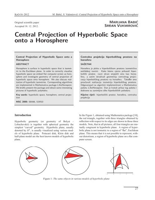
In the Figure 1, obtained using Mathematica package [10],
the red triangle, together with three triangles obtained by
reflection with respect to its edges are shown in those three
models. Note, that in all pictures, all four triangles are mutually
congruent in hyperbolic plane. A region of hyperbolic
plane is not isometric to a region of “flat”, Euclidean
plane. This means that it is not possible to represent, without
distortions, a region of hyperbolic plane on a flat computer
screen.
4
3
2
1
Figure 1: The same objects in various models of hyperbolic plane
-1 0 1 2 3
27

KoG • 16–2012
M. Babić, S. Vukmirović: Central Projection of Hyperbolic Space onto a Horosphere
Therefore, hyperbolic metric of model is not inherited from
the Euclidean plane: distances become infinitely big near
absolute (unit circle in the first two models and x-axis in
the third model). Although to our eyes the absolute is finite,
it represents infinity of the hyperbolic plane.
For hyperbolic space H 3 there exist analogous models:
Poincaré ball, Klein ball and half-space model. Two approaches
for visualization of the hyperbolic space have
been used so far, and both approaches at least in one instance
use some model.
The first is to represent a geometrical object in some model
of hyperbolic space in R 3 and then to project it onto computer
screen by standard central projection of R 3 . This
approach was used in the famous movie Not knot ([6]).
This is also used a popular way of visualizing large graph
objects and the structure of world wide web (see [7] and
others). Probably the most famous visualizations of hyperbolic
space so far are done by J. R. Weeks ([11, 12]) and
use this approach.
The second approach is to fix a hyperbolic plane H 2 in hyperbolic
space L 3 , project the space onto H 2 by means of
central projection in L 3 and finally visualize the plane H 2
using some model on the computer screen. In the master
thesis [1] the author develops ray tracing algorithm for hyperbolic
space and uses this approach for visualization.
In this paper we take a different approach. We wonder:
how would hyperbolic space look like to us, if we were
there? Equivalently, in terms of computer graphics: how
would the picture look like if we isometrically embed our
flat computer screen into H 3 , project the hyperbolic space
on the screen by means of central projection in H 3 and then
watch the picture on the screen without any distortions and
models?
The mathematical answer was well known to very founders
of hyperbolic geometry: there is a peculiar surface in
H 3 , called horosphere, which is isometric to Euclidean
plane. Therefore, if we isometrically embed a flat, Euclidean
screen in hyperbolic space it may become a part of
horosphere. In this paper we discuss necessary mathematical
background regarding central projection of hyperbolic
space onto horosphere, as well as, isometric transformations
of the hyperbolic space. The final result is Mathematica
package L3toHorosphere that allows visualization
of H 3 by means of central projection onto horosphere and
also visualization of hyperbolic motions. Using this package
many interesting pictures and animations are obtained
(see [3]).
On our request, Prof. Emil Molnár informed us that Prof.
Imre Juhász (the head of Department of Descriptive Geometry
of the University of Miskolc) dealt with a similar
topic in his awarded Scientific Student Circle (OTDK) paper
(in 1979) and in his diploma work (1978) at the Debrecen
University, without any scientific publication on this
topic, later on.
It is also worth mentioning that methods of Descriptive
geometry in hyperbolic space have also been investigated
(see [8, 9]).
Description of hyperbolic isometries is mathematically
simple and found in many classical books, but when it
comes to practical implementation the paper [5] is usually
used. In this work we briefly cover this topic using slightly
different approach that someone may find easier to understand.
The paper is organized as follows. In the first section we
give a brief overview of models of hyperbolic space. In the
second section we study horosphere and central projection
onto horosphere. The third section is devoted to implementation
of isometries of hyperbolic space. In the fourth
section we give some examples of projections and animations
obtained using package L3toHorosphere. In the last
section we compare various approaches in visualizing hyperbolic
geometry and give some ideas for future work.
Authors would like to thank Prof. Emil Molnár for useful
discussions and for careful reading which significantly
improved the final version of the paper.
1 Models of hyperbolic space
1.1 Klein ball and projective model
Klein ball model {P(x,y,z)|x 2 + y 2 + z 2 < 1} is interior of
unit sphere in R 3 . The unit sphere is absolute of this model.
This means that points of unit sphere represent points in infinity
of the hyperbolic space. Hyperbolic lines and planes
are parts of Euclidean lines and planes. The distance between
points P and Q is given by the formula
d(P,Q) = 1 |QA||PB|
log
2 |PA|QB| , (1)
where A and B are endpoints of the chord containing P and
Q and | · | denotes the Euclidean distance.
Klein ball model is closely related to Klein projective
model or pseudosphere model. Namely for point P(x,y,z)
from the Klein model, one can consider homogenous coordinates
P(x : y : z : 1). There are unique coordinates
¯P(x 1 ,x 2 ,x 3 ,x 4 ) representing the same point and satisfying
the relation
−x 2 1 − x 2 2 − x 2 3 + x 2 4 = 1, x 4 > 0. (2)
This means that one can regard hyperbolic space as pseudosphere
(2) in Minkowski vector space R (3,1) , with inner
product · given by matrix J = diag(−1,−1,−1,1).
28

KoG • 16–2012
M. Babić, S. Vukmirović: Central Projection of Hyperbolic Space onto a Horosphere
It is interesting that formula (1) for distance translates into
d(P,Q) = cosh −1 ( ¯P · ¯Q),
where ¯P(x 1 ,x 2 ,x 3 ,x 4 ) and ¯Q(y 1 ,y 2 ,y 3 ,y 4 ) are coordinates
of these points. Therefore, the isometries of Klein projective
model are those projective transformations that preserve
the pseudosphere, i.e. the inner product given by
matrix J. The importance or this model is its linear nature:
the lines and planes are linear and isometries are represented
as multiplication of vectors by 4 × 4 matrices that
belong to classical linear group SO(3,1).
1.2 Half-space model
Half-space model consists of all points P(x,y,z) from R 3
satisfying the relation z > 0. The plane z = 0 is absolute
of this model. Hyperbolic lines are half-circles orthogonal
to the absolute (i.e. with center on the absolute and lying
in a plane orthogonal to the absolute) and Euclidean rays
orthogonal to the absolute. Planes of this model are halfspheres
and half-planes orthogonal to the absolute. To be
mathematically correct, we add single infinite point P ∞ to
R 3 . This point compactifies R 3 to sphere S 3 whereas the
absolute z = 0 becomes two-dimensional sphere, like absolute
in the other two models. Each plane and each line
in R 3 can be regarded as sphere and circle, containing P ∞ .
The distance in this model is best described using the metric
tensor
ds 2 = dx2 + dy 2 + dz 2
z 2 . (3)
The isometries are compositions of reflections and inversions
with respect to hyperbolic planes. We are interested
in half-space model since the horosphere has its simplest
representation in this model, as we show in the sequel.
1.3 Poincaré ball model
Poincaré ball model {P(x,y,z)|x 2 + y 2 + z 2 < 1} is the interior
of unit sphere in R 3 . The unit sphere is absolute of
this model. Hyperbolic Lines are parts of circles orthogonal
to the absolute and parts of lines orthogonal to the absolute
(i.e. passing through the origin). Hyperbolic planes
are parts of spheres orthogonal to the absolute and parts of
planes orthogonal to absolute. The metric tensor reads
ds 2 = dx2 + dy 2 + dz 2
(1 − x 2 − y 2 − z 2 ) 2 .
The isometries are compositions of reflections and inversions
with respect to hyperbolic planes. The mapping
f(x,y,z) = (2(x,y,z))/(1+x 2 + y 2 + z 2 ) (4)
is isometry that maps point P(x,y,z) from Poincaré to
Klein model. Isometry between Poincaré ball model and
half-space model is simple composition of translations and
spherical inversion
g(x,y,z) =
1
x 2 + y 2 +(z − 1) 2(4x,4y,2(1 − x2 − y 2 − z 2 )).
2 Horosphere and the related central projection
2.1 Horosphere
Fix a point O on absolute and point M ∈ H 3 . Horosphere
(with center O containing point M) is set of images of point
M in reflections with respect to all planes containing O.
Note that, if O is finite point and M ′ is image of M then
OM is congruent to OM ′ and the horosphere is hyperbolic
sphere with center O. Therefore, one may think of horosphere
as of sphere with center in infinity.
From construction of horosphere it follows that all horospheres
are mutually congruent in H 3 . We want to find the
the simplest one in some model. Consider point P ∞ of the
half-plane model as center of horosphere, and any finite
point M(x 0 ,y 0 ,z 0 ) of that model. All hyperbolic planes
through P ∞ are exactly all Euclidean half-planes orthogonal
to the absolute z = 0. Therefore, all images M ′ of
M have the same z−coordinate and the horosphere is the
plane z = z 0 . Note that this special horosphere touches the
absolute in point P ∞ . Since isometries are compositions
of inversions and reflections, all horospheres of half-space
model are Euclidean spheres that touch the absolute in its
center, or planes parallel to the absolute.
From the isometries (4) and (5) between models we conclude
that horospheres in Poincaré ball model are spheres
touching the absolute in their center and in Klein ball
model ellipsoids touching the absolute. The most simple
horosphere z = z 0 in half-space model has restriction of
the metric tensor (3) equal to
ds 2 = dx2 + dy 2
z 2 ,
0
showing that the horosphere is isometric to the Euclidean
plane, up to a scale. Since in this case the isometry between
horosphere and Euclidean plane is given by the imbedding
itself, the setup consisting of half-space model and horosphere
z = z 0 is the one we use for implementation of the
central projection.
Reparameterizing, one can write metric (3) in the form:
ds 2 = e 2t (
k dx 2 + dy 2) + dt 2 ,
(5)
29

KoG • 16–2012
M. Babić, S. Vukmirović: Central Projection of Hyperbolic Space onto a Horosphere
where k > 0 is the the curvature constant (in our case
k = 1). This is so called horospherical coordinate system
of the hyperbolic space H 3 , which consists of “concentric”
horospheres, parameterized by the real line, t ∈ R.
In each horosphere we have Euclidean plane coordinates
(x,y). This was the basic idea for distance measure of János
Bolyai in his absolute geometry (in nowadays formulation,
Lobachevskii distinguished the non-Euclidean case from
the beginning), introduced without any model.
2.2 Central projection onto horosphere
We have shown that we can embed flat computer screen
into hyperbolic space as a part of horosphere. What would
an observer see on the screen if he is in the hyperbolic
space? In any geometry, light ray carrying visual information
from the object to the eye of the observer travels
along geodesic, i.e. along straight line of that geometry.
Klein model is the the easiest to sketch, since the hyperbolic
lines of that model are parts of Euclidean lines. If we
place the observer O outside the horosphere (see Figure 2,
left) some points cannot be projected (point N) while others
have two possible projections along the light ray (point
M). On the other hand, if we place the observer inside the
horosphere (see Figure 2, right) the projection is well defined
for all points of hyperbolic space. For this reason, we
chose that observer is inside the horosphere, although it is
possible to consider the other case.
The line segment is projected into intersection of horosphere
and the hyperbolic plane determined by the center
of projecection O and the segment. For our purposes it is
sufficient to consider half-space model, horosphere z = z 0
and the point O(0,0,ω),ω > z 0 .
Recall that hyperbolic line segment is either Euclidean segment
orthogonal to the absolute or circular arc orthogonal
to the absolute. The following cases are possible:
1. If hyperbolic segment is circular arc AB then hyperbolic
plane containing A,B and O is half-sphere. The
projection of the segment belongs to intersection of
the half-sphere and the horosphere. It is circular arc
A ′ B ′ in horosphere z = z 0 (see Figure 3).
2. If hyperbolic segment is an Euclidean segment AB
orthogonal to absolute then the hyperbolic plane
OAB is Euclidean half-plane. The central projection
of segment AB is
a) Euclidean segment A ′ B ′ if segment AB have no
common point with z−axis above O (that is
point (0,0,z),z > ω;
b) Euclidean ray starting from A ′ if B is of form
B(0,0,z),z > ω. This ray belongs to the intersection
line of α and horosphere;
c) Two disjoint Euclidean rays starting from A ′
and B ′ and belonging to the intersection line of
α and horosphere. This happens if segment AB
has one inner point of the form (0,0,z),z > ω;
d) Empty set if segment AB is contained in the set
{(0,0,z)|z > ω}.
Figure 2: Observer outside and inside the horosphere.
In the half-space model, the point O(x,y,z) is inside the
horosphere z = z 0 if the condition z > z 0 holds. Particular
coordinates of point O doesn’t matter, so we can chose
O(0,0,ω), ω > z 0 .
Note that all points of half-space model are projected into
finite points of horosphere z = z 0 , except points M of the
form M(0,0,z),z > ω that are projected into point P ∞ , the
infinite point of the horosphere (i.e. screen).
2.3 Central projection of hyperbolic line segment
In order to visualize polyhedra in hyperbolic space we have
to understand the projection of hyperbolic line segment.
Figure 3: Central projection of hyperbolic line segment.
Note that that there are two circular arcs in horosphere
z = z 0 with endpoints A ′ and B ′ . Therefore, to determine
uniquely the projection of segment AB we need the projection
C ′ of some point C belonging to the segment AB.
Similar holds for Euclidean ray with the endpoint A ′ .
30

KoG • 16–2012
M. Babić, S. Vukmirović: Central Projection of Hyperbolic Space onto a Horosphere
2.4 Visibility
We assume that polyhedra consists of faces that are not
transparent. Therefore, not all vertices and edges are visible
from the center of projection O. We may draw nonvisible
edges as dashed lines to improve spacial understanding
of the polyhedra (see for example Figure 5). Visibility
in Klein ball model coincides with Euclidean visibility.
Therefore, to determine the visibility one can use the standard
algorithms from R 3 .
In reality, the human eye sees the part of scene that is inside
the cone of vision. In computer graphics this translates into
clipping. In this work we don’t mind about cone of vision
and consider mathematical central projection of polyhedra,
i.e. we project points at the front, as well as, at the back of
the observer. However, in our package [4] there is an option
to draw the circle that separates front and back of the
observer. That circle is the intersection of half-sphere with
center (0,0,0) and radius ω and horosphere z = h < ω.
In Figure 11 (a) this is the black circle. The observer is
inside the blue cube, so all its edges are visible, but some
part of the cube is in the front and some part is in the back
of the observer.
3 Isometries of hyperbolic space
The isometries of hyperbolic space are mathematically
well known. The fastest and most elegant way to implement
the isometries is to represent them as 4 × 4 matrices
that are applied to column vectors of homogenous coordinates
of points in Klein projective model. The homogenous
coordinates are of the form P(x 1 : x 2 : x 3 : x 4 ), where homogeneity
means that coordinates (λx 1 : λx 2 : λx 3 : λx 4 ),
for each λ ≠ 0 represent the same point.
As explained in Subsection 1.1 the isometries of Klein
model belong to linear group SO(3,1). They are linear
mappings preserving Minkowski inner product, i.e. matrix
A of an isometry satisfies A T JA = J, where J =
diag(−1,−1,−1,1) is diagonal matrix of the inner product.
Any hyperbolic isometry is composition of less than
four reflections with respect to hyperbolic planes. In this
review we don’t want to exhaust all isometries, so we
present only isometries that are composition at most two
plane reflections.
The plane has normal vector n α = (α 1 : α 2 : α 3 : −α 4 ) T
with respect to the inner product given by matrix J. One
can show that the reflection S α with respect to the plane α
has the matrix
S[n α ] = I 4 − 2 n αn α T J
n α T Jn α
, (6)
where I 4 is 4 × 4 identity matrix. It is important to note
that the numerator n α n T αJ is 4 × 4 matrix, while denominator
n T αJn α is squared norm of vector n α and therefore a
number. Vector n α is considered column, while n T α is row
vector.
Figure 4: Cube and its reflections.
The Figure 4 shows consecutive reflections of the blue
cube with respect to the opposite faces (red cubes).
One can show that reflection S[P] with respect to point
P(x 1 : x 2 : x 3 : x 4 ) is given by the matrix
S[P] = I 4 − 2 PPT J
P T JP ,
which uses the same formula as the reflection 6 with respect
to hyperplane. The reflection S[P] is formally defined
as composition of three reflections S[γ] ◦ S[β] ◦ S[α]
with respect to three mutually orthogonal planes α,β and γ
that intersect in the point P.
The Figure 5 represents the red cube and its reflection with
respect to its vertex.
3.1 Reflection with respect to plane (or point)
Plane in the Klein projective model is represented by hyperplane
in the vector space R (3,1) , so it has an equation
α 1 x 1 + α 2 x 2 + α 3 x 3 + α 4 x 4 = 0
Figure 5: Central reflection of a cube.
31

KoG • 16–2012
M. Babić, S. Vukmirović: Central Projection of Hyperbolic Space onto a Horosphere
3.2 Translation
Translation is composition S[β] ◦ S[α] of two reflections
with respect to hyperparallel planes α and β, i.e. the planes
that have common normal line n, (that line is unique in hyperbolic
geometry). If A and B are intersections of n with
α and β, respectively, we call it translation from A to B
and denote it T[AB]. Note that T[AB] is not translation by
vector AB, since the notion of vector is not possible to define
in hyperbolic geometry. Many other properties of hyperbolic
translation are quite different from its Euclidean
counterpart. For example, we have T[AB](A) = B and if
T[AB](M) = N then hyperbolic segments AB and MN are
not congruent if M ≠ A. Moreover, the relation AB ≤ MN
always hold.
This is illustrated in Figure 6 which represent translation
of a cube along its edge, i.e. form one vertex to another.
Unlike in the Euclidean case, the face of the cube is not
translated to the opposite face.
a
Figure 7: Dodecahedron and its translates.
3.3 Rotation
Hyperbolic rotation is composition R[p,φ] = S[β] ◦ S[α] of
two reflections with respect to planes that intersect along
axes of rotation, the line p = α ∩ β, and the angle between
α and β equals φ 2
. From formula (1) it follows that Euclidean
rotations that fix the origin O(0,0,0) are also hyperbolic
rotations. The consequence is that the angles in
the origin of the Klein ball model are the same as Euclidean
angles (this doesn’t hold for any other point of Klein ball
model). Therefore, to perform the rotation about line p,
translate p to the origin, rotate around translated line p ′ as
Euclidean rotation and finally translate back. To be more
specific, if Q ∈ p is any point of p, then R[p,φ] is given by
the matrix:
R[p,φ] = T[OQ] ◦ R[p ′ ,φ] ◦ T[QO],
where homogenous coordinates of the origin are O(0 : 0 :
0 : 1), p ′ = T[QO][p], and R[p ′ ,φ] is 4 × 4 matrix
(
R[p ′ R
,φ] =
E [p ′ )
,φ] 0
.
0 1
Here we denote by R E [p ′ ,φ] the 3 × 3 Euclidean matrix of
rotation around Euclidean line p ′ by angle φ.
Figure 6: Central projection of cube and its translate.
b
To find matrix of translation denote by C the hyperbolic
midpoint of segment AB. One can show that T[AB] =
S[β] ◦ S[α] = S[C] ◦ S[A] and hence its matrix is product of
known matrices:
T[AB] = S[C]S[A].
To find the hyperbolic midpoint C of the segment AB one
can use the formula:
C = A
√
(B T JB)(A T JB)+B
√
(A T JA)(A T JB).
Figure 8: Consecutive rotations of regular octahedron.
32

KoG • 16–2012
M. Babić, S. Vukmirović: Central Projection of Hyperbolic Space onto a Horosphere
3.4 Limit rotation
4 Mathematica package L3toHorosphere
The limit or horocyclic rotation is probably the most intriguing
isometry of hyperbolic plane, since it doesn’t exist
in Euclidean geometry. Limit rotation is composition
S[β]◦S[α] of two reflections with respect to parallel hyperbolic
planes α and β, i.e. the planes with single common
point on the absolute.
Mathematica package L3toHorosphere has three main features:
• central projection of hyperbolic polyhedra onto
horosphere;
• visualization of the polyhedra and its projection in
half-space model;
• realization of isometries of hyperbolic space.
Figure 9: Horocylic rotation in the Klein ball model.
We now describe general formulas of limit rotation. Note
that parallel planes α and β in Klein ball model are parts of
Euclidean planes α and β that intersect along line q touching
the absolute in point P(x 0 ,y 0 ,z 0 ) (see Figure 9).
Planes α and β have normal vector of the form
Within the package, user can define any polyhedral surface
in hyperbolic space by defining its faces (as lists of vertices)
and vertices (using coordinates in any model). The
polyhedral surface than can be repositioned using various
hyperbolic isometries. Finally, the projection of the polyhedral
surface onto horosphere can be obtained (see figures
from Section 3).
Pcosφ+(q × P)sinφ = (a 1 (φ),a 2 (φ),a 3 (φ)),
for some φ = φ α ,φ = φ β . One can show that the normal
vector of these planes in R (3,1) in homogenous coordinates
is given by:
n(φ)=(a 1 (φ) : a 2 (φ) : a 3 (φ) : a 1 (φ)x 0 +a 2 (φ)y 0 +a 3 (φ)z 0 ).
Now, the 4 × 4 matrix of the limit rotation S[β]◦S[α] is the
product S[n(φ β )]S[n(φ α )] of their reflection matrices.
In the Figure 10 a horocyclic rotation is consecutive applied
on the blue cube in both directions. One can imagine
that “small” cubes converge to a single point in infinity -
the center of horocyclic rotation. Of course, all the cubes
are congruent but the cubes further from the observer appear
smaller.
a
b
Figure 10: Horocylic rotation applied on cube.
Figure 11: Observer inside a cube: a) projection,
b) situation in the half-space model.
To achieve better understanding of what’s going on, user
can also visualize the polyhedral surface and its projection
onto horosphere in the half-space model (see Figure 11).
Visibility is implemented only for convex polyhedra without
boundary.
33

KoG • 16–2012
M. Babić, S. Vukmirović: Central Projection of Hyperbolic Space onto a Horosphere
Now we only list the functions implemented in the package.
Some functions have options that can be obtained using
commandOptions[function]. More details can be
found in the user guide file that is delivered with the package
[4].
drawProjection[ω, k, vert, faces, options]
- project polyhedra given by faces and vertex coordinates
vert from point O(0,0,ω) onto horosphere
z = k,ω > k.
modelHS[ω, k, vert, faces, options] - in
half-space model draws polyhedra given by faces
and vertex coordinates vert and its central projection
from point O(0,0,ω) onto horosphere z = k,ω > k).
reflect[nVector] - returns 4×4 matrix of reflection
with respect to plane α with normal vector nVector.
The normal vector is given in homogenous coordinates,
i.e. is list of 4 numbers.
reflect[P] - returns 4 × 4 matrix of reflection with
respect to point P given in homogenous coordinates.
translate[A,B] - returns 4 × 4 matrix of translation
from A to B.
rotate[A,B][φ] - returns 4 × 4 matrix of rotation by
angle φ around line AB.
limitRotate[P][p][φ] - returns 4 × 4 matrix of
limit rotation by “angle” φ ≠ π 2
(modπ) around line
with direction p and containing unit point P (P orthogonal
to p). The points P and p are given in the form
(x,y,z).
Klein2HS[pt] - converts Klein projective pointpt of
form (x 1 : x 2 : x 3 : x 4 ) to half-space model.
HS2Klein[pt] - converts half space point pt of the
form (x,y,z),z > 0 to Klein projective point.
m[A,B] - returns midpoint of segment AB. All points
are in Klein projective coordinates (x 1 : x 2 : x 3 : x 4 ).
normalVector[pt1, pt2, pt3] - returns projective
normal vector of plane determined by three points. All
points are in Klein projective coordinates (x 1 : x 2 : x 3 :
x 4 ).
edges[faces] - returns edges of polyhedra with faces
given byfaces.
The sum of the angles in a hyperbolic triangle is strictly
less than π. Therefore, when sketching hyperbolic objects
we usually draw them to be curved concave. However, the
projections we get in this paper are curved convex, what
may bother someone’s intuition. It is interesting that if the
observer is placed outside the horosphere (first picture in
Figure 2) the projections become curved concave. The Figure
12 (a) shows projection of a cube obtained using this
approach.
It would be interesting to implement horosperical central
projection of hyperbolic space in some more efficient programming
language than Mathematica. This would allow
us rendering of more complex hyperbolic scenes and probably
lead to very interesting and unusual pictures. However,
we are of opinion that even basic Mathematica package
[4] we developed, can be very useful for better understanding
of hyperbolic geometry and can be used as a good
starting point for more complex visualizations.
One of classical scenes is Figure 12 (b), from video Not
knot ([6]), used to cover many mathematical books. It represents
tiling of hyperbolic space with regular dodecahedrons.
This classic idea is common inspiration in mathematical
art and jewelry making (see [2]). The natural
question is to see regular hyperbolic tilings rendered using
horospherical central projection.
a
5 Conclusion and future work
The main advantage of our horosperical projection are realistic
images of hyperbolic space. As in Euclidean central
projection, closer objects appear larger. Furthermore, we
don’t use models of particular parameterizations - our projections
are geometrically invariant and represent what flat
Euclidean eye would really see in the hyperbolic space.
All other approaches “cheat” in some way. The inevitable
drawback of our approach is that projection of hyperbolic
segment, in generic case, is circular arc that is complex to
render. However, this is not heavy task for modern computers.
b
Figure 12
Another interesting topic is stereoscopic vision of hyperbolic
scenes investigated in the paper [11]. Our preliminary
testing, surprisingly, gave positive results, i.e. the human
visual system seems to be able to “see” in hyperbolic
space.
34

KoG • 16–2012
M. Babić, S. Vukmirović: Central Projection of Hyperbolic Space onto a Horosphere
References
[1] B. AJDIN, Rejtrejsing u Poenkareovom sfernom modelu
hiperboliˇckog prostora, master thesis, Faculty
of Mathematics, Belgrade, 2010, (in Serbian, sort
english version available at http://www.mpi-inf.
mpg.de/~bajdin/HRayTracing-eng.pdf,
acessed august 2012.)
[2] V. BULATOV, Tilings of the hyperbolic space and
their visualization, Joint MAA/AMS meeting, New
Orleans, 2011. (available at//bulatov.org/math/
1101/, acessed august 2012.)
[3] M. BABIĆ, Vizualizacija prostora Lobaˇcevskog,
master thesis, Faculty of Mathematics, Belgrade,
2010, (in Serbian, available athttp://alas.matf.
bg.ac.rs/~vsrdjan/files/marijana.pdf,
acessed august 2012.)
[4] M. BABIĆ, S. VUKMIROVIĆ, L3toHorosphere - central
projection of hyperbolic space onto horosphere,
Mathematica package 8335, Mathsource, 2012.
[5] M. PHILLIPS, C. GUNN, Visualizing hyperbolic
space: Unusual uses of 4 × 4 matrices,, Proc. 1992.
Symp. Interactive 3D Graphics, ACM Press, New
York, 1992, 209–214.
[6] C. GUNN, D. MAXWELl, Not knot, video, 16 minutes,
1995.
[7] T. MUNZNER, Exploring Large Graphs in 3D Hyperbolic
Space, IEEE Computer Graphics and Applications
18 (4) (1998), 18–23.
[8] Z. A. SKOPEC, “Foundations of Descriptive Geometry
of Hyperbolic Space” (Russian), series
“Metods of Descrptive Geometry and its Applications”,
Moscow, 1955.
[9] Z. ŠNAJDER, Gemeinsame Eigenschaften der zentralen
normalen, parallelen und berparallelen Projektionen
im dreidimensionalen hyperbolischen Raum
(German), Mat. Vesnik 9(24) (1972), 27–37.
[10] S. VUKMIROVIC, L2Primitives - basic drawing in
the hyperbolic plane, Mathematica package, 1998,
http://library.wolfram.com/infocenter/
MathSource/4260/
[11] J. R. WEEKS, Real-time rendering in curved spaces,
IEEE Computer Graphics and Applications 22 (6)
(2002), 90–99.
[12] J. R. WEEKS, Real-time animation in hyperbolic,
spherical, and product geometries, Non-Euclidean
Geometries, János Bolyai Memorial Volume, (Ed. A.
Prékopa and E. Molnár), Mathematics and its Applications
581, Springer, 287–305, 2006.
Marijana Babić
e-mail: marijana@matf.bg.ac.rs
Srdan Vukmirović
e-mail: vsrdjan@matf.bg.ac.rs
Faculty of Mathematics, University Belgrade
Studentski trg 16, Belgrade, Serbia
35