REYKJAVÍK, ICELAND AUGUST 11-13, 2008 - Veðurstofa Íslands

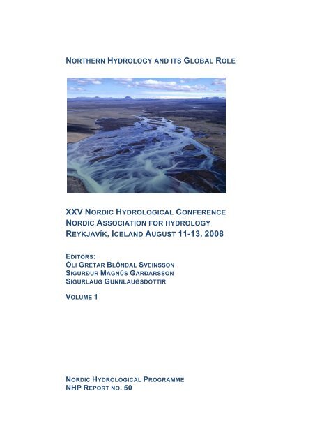
NORTHERN HYDROLOGY AND ITS GLOBAL ROLE
XXV NORDIC HYDROLOGICAL CONFERENCE
NORDIC ASSOCIATION FOR HYDROLOGY
REYKJAVÍK, ICELAND AUGUST 11-13, 2008
EDITORS:
ÓLI GRÉTAR BLÖNDAL SVEINSSON
SIGURÐUR MAGNÚS GARÐARSSON
SIGURLAUG GUNNLAUGSDÓTTIR
VOLUME 1
NORDIC HYDROLOGICAL PROGRAMME
NHP REPORT NO. 50

THIS PUBLICATION IS A CONTRIBUTION OF ICELAND TO THE 7TH PHASE
OF THE INTERNATIONAL HYDROLOGICAL PROGRAMME, UNESCO’S
INTERGOVERNMENTAL SCIENTIFIC PROGRAMME IN WATER RESOURCES,
SPONSORED THROUGH THE ICELANDIC HYDROLOGICAL COMMITTEE

NORTHERN HYDROLOGY AND ITS GLOBAL ROLE
XXV NORDIC HYDROLOGICAL CONFERENCE
NORDIC ASSOCIATION FOR HYDROLOGY
REYKJAVÍK, ICELAND AUGUST 11-13, 2008
EDITORS:
ÓLI GRÉTAR BLÖNDAL SVEINSSON
SIGURÐUR MAGNÚS GARÐARSSON
SIGURLAUG GUNNLAUGSDÓTTIR
VOLUME 1
NORDIC HYDROLOGICAL PROGRAMME
NHP REPORT NO. 50

Northern Hydrology and its Global Role
Editors:
Óli Grétar Blöndal Sveinsson
Sigurður Magnús Garðarsson
Sigurlaug Gunnlaugsdóttir
Reykjavik 2008
Icelandic Hydrological Committee
Grensásvegur 9
IS 108 Reykjavik
Iceland
Volume 1
ISBN 978-9979-68-238-7
Nordic Hydrological Programme
NHP Report no. 50

LIST OF CONTENTS
VOLUME 1
Preface ........................................................................................................... 9
Plenary Session 1 ....................................................................................... 11
Arne Tollan: Northern Hydrologists And Their Global Roles ................... 13
Upmanu Lall: Climate Change And Variability: How Can We Inform
Strategies For Adaptation ............................................................................ 32
André Musy & René Roy: Nordic Hydrology In Climate Change Context:
The Ouranos Experience In Québec ........................................................... 33
Sveinn T. Thorolfsson: Urban Hydrology And Sustainable Urban Drainage
At Lake Urridavatn In Gardabaer, Iceland .................................................. 34
Session 2: Arctic Hydrology And Glaciers ............................................. 45
Valery Vuglinsky: Changes In Ice Regimes Of Rivers In The Northern Part
Of European Russia ..................................................................................... 47
Thorsteinn Thorsteinsson, Arni Snorrason, Charles Vörösmarty & Jonathan
Pundsack: Arctic HYDRA: The Arctic Hydrological Cycle Monitoring
And Assessment Program ........................................................................... 54
Arvid Bring & Georgia Destouni: Spatial Patterns Of Decline In Pan-Arctic
Hydrological Monitoring Networks: A Vulnerability Map ........................ 60
Jan Magnusson, Tobias Jonas, Ignacio López-Moreno & Michael Lehning:
Potential Impact Of Climate Change On The Snowpack In A Partly-
Glaciated Basin In Central Switzerland ...................................................... 67
Hrund Ó. Andradóttir: Thermal Dynamics Of Sub-Arctic Lake Lagarfljót,
Iceland ......................................................................................................... 82
Bergur Einarsson, Thorsteinn Thorsteinsson & Tómas Jóhannesson: The
Initiation And Development Of A Jökulhlaup From The Subglacial Lake
Beneath The Western Skaftá Cauldron In The Vatnajökull Ice Cap, Iceland
................................................................................................................ 94
Peter F. Rasmussen, Sung Joon Kim & Woonsup Choi: Hydrologic
Modeling Of Two Canadian Watersheds Using The North American
Regional Reanalysis Data ......................................................................... 102
3

Tobias Jonas, Manfred Stähli & David Gustafsson: Radiation Budget In A
Snow-Covered Subalpine Forest And Its Interactions With The Snowpack ..
.............................................................................................................. 112
Inese Mikelsone, Élise Lépy & Yuriy Shishkin : Ice And Weather
Conditions In The Gulf Of Riga, Their Impact On Riga Harbor Winter
Navigation, 1996-2006 .............................................................................. 113
Markku Puupponen: Towards Integrated Systems For Arctic Hydrology –
Applications At The Finnish Hydrological Service .................................. 121
Benjamin A. Black & Thorsteinn Thorsteinsson: Processes And
Morphologies Of Icelandic Gullies And Implications For Mars .............. 124
Session 3: Water Resources Management Under Climate Change ... 133
Agrita Briede & Lita Lizuma: Long-Term Records Of Precipitation In
Latvia ......................................................................................................... 135
Helen K. French, Kristine Flesjø, Jarl Øvstedal, Hans-Olav Eggestad &
Heidi Grønsten: Climate Change And Pollution Risks Related To
Infiltration In Partially Frozen Soils ......................................................... 143
Astrid Voksø, Nils Kristian Orthe, Hege Hisdal & Kolbjørn Engeland: Low
Flow Index Map For Norway – Interaction Using GIS-Software And
Analysis ..................................................................................................... 154
Johanna Korhonen: Long-Term Changes In Discharge Regime In Finland ..
.............................................................................................................. 160
Elga Apsīte, Anda Bakute & Ilze Rudlapa: Climate Change Impacts On
The Total Annual Rivers’ Runoff Distribution, High And Low Discharges
In Latvia .................................................................................................... 171
Deborah Lawrence, Stein Beldring, Ingjerd Haddeland & Thomas
Væringstad: Integrated Framework For Assessing Uncertainty In
Catchment-Scale Modelling Of Climate Change Impacts: Application To
Peak Flows In Four Norwegian Catchments ............................................. 182
Jannes Stolte & Helen French: Overland Flow Induced By Snowmelt,
Effects Of Climate Change ....................................................................... 191
Elga Apsite, Ansis Ziverts & Anda Bakute: Study Of Hydrological
Processes For Development Of Mathematical Model METQ .................. 200
Ingjerd Haddeland: Modelling Of Current And Future Water Resources In
Northern Europe ........................................................................................ 210
Sveinn T. Thorolfsson, Asle Aasen, Magnar Sekse & Olav Totland:
Research And Implementation Of Alternative Stormwater Management In
The City Of Bergen, Norway 1981 – 2008 ............................................... 212
4

Session 4: Uncertainty And Extremes In Hydrology ........................... 221
Emiliano Gelati, Ole Bøssing Christensen, Peter Rasmussen & Dan
Rosbjerg: Down-Scaling Atmospheric Patterns To Multisite Precipitation
Amounts In Southern Scandinavia ............................................................ 223
Ólafur Rögnvaldsson: Dynamical Downscaling Of Precipitation – Part I:
Comparison With Glaciological Data ....................................................... 236
Ólafur Rögnvaldsson: Dynamical Downscaling Of Precipitation – Part II:
Comparison With Rain Gauge And Hydrological Data ........................... 244
Wei Yang, Johan Andréasson, L. Phil Graham, Jonas Olsson, Jörgen
Rosberg & Fredrik Wetterhall: A Scaling Method For Applying RCM
Simulations To Climate Change Impact Studies In Hydrology................ 256
Asgeir Petersen-Øverleir: The Net Effect Of Sample Variability & Rating
Curve Imprecision In Regional Flood Frequency Analysis ...................... 266
Snorri Árnason: Estimating Bayesian Rating Curves For The Icelandic
Hydrometric Network ............................................................................... 275
Olga Kovalenko & Anna Põrh: Flood Risk Of Coastal Areas Tallinn And
Pärnu .......................................................................................................... 286
Sveinn T. Thorolfsson, Lars Petter Risholt, Olav Nilsen, Andreas
Ellingsson, Vidar Kristiansen, Øystein Hagen & Edgar Karlsen: Extreme
Rainfalls And Damages On August 13 2007 In The City Of Trondheim,
Norway ...................................................................................................... 295
Bogi Brynjar Björnsson, Esther Hlíðar Jensen, Inga Dagmar Karlsdóttir &
Jórunn Harðardóttir: On The Road To A New National Hydrological
Database Of Iceland .................................................................................. 302
Kristinn Már Ingimarsson, Birgir Hrafnkelsson, Sigurdur Magnús
Garðarsson & Árni Snorrason: Bayesian Estimation Of Discharge Rating
Curves ........................................................................................................ 308
VOLUME 2
Session 5: Advanced Methods And Technologies In Hydrological
Practice ..................................................................................................... 327
Hervé Colleuille, Stein Beldring, Zelalem Mengistu, Lars Egil Haugen,
Trude Øverlie, Andersen Jess & Wai Kwok Wong: Monitoring System For
Groundwater And Soil Water Based On Simulations And Real-Time
Observations: The Norwegian Experience ............................................... 329
5

Sten Bergström & Gunlög Wennerberg: The Swedish Hydrological Service
During 100 Years ...................................................................................... 340
Yisak Abdella & Knut Alfredsen: Integration Of Radar Precipitation In
Distributed Hydrological Modelling ......................................................... 351
Søren Elkjær Kristensen & Ivar Olaf Peereboom: Identification Of Areas
Exposed To Flooding In Norway At A National Level ............................ 363
Uldis Bethers, Juris Seņņikovs & Andrejs Timuhins: Employment Of
Regional Climate Models As Data Source For Hydrological Modelling . 373
Péter Borsányi & Paul Christen Røhr: Development Of Dynamic Flood
Forecasting Services .................................................................................. 384
Kristoffer Dybvik, Erlend Moe & Andre Soot: Discharge Comparison
Measurements, Ice Covered Rivers ........................................................... 394
Wolfram Sommer & Benno Wiesenberger: RQ-24 Non-Contact Discharge
Measurement ............................................................................................. 400
Wolfram Sommer, Reinhard Fiel & Benno Wiesenberger: Snow Water
Sensor (SWS) To Measure Snow Water Equivalent (SWE) And Liquid
Water Content ........................................................................................... 411
Christer Jonsson & Markus Andersén: Hydro Acoustic Measurement
Techniques All The Way – Consequences And Experiences ................... 421
Cristina Alionte Edlund: Preview/Northern Flood Forecasting Service A
Modern Flood Forecasting Service For Better Risk Management ........... 427
Ivar Olaf Peereboom: Dynamic Flood Mapping ....................................... 430
Kai Rasmus, Antti Lindfors & Mikko Kiirikki: On The Applicability Of A
3D Hydrodynamic Model For The Calculation Of Currents In Local
Coastal Sea Area... .................................................................................... 435
Laufey Bryndís Hannesdóttir & Óli Grétar Blöndal Sveinsson: The Water
Resources Database At Landsvirkun ........................................................ 442
Session 6: Hydro Power And Hydrology .............................................. 453
Karen Lundholm, Barbro Johansson, Eirik Malnes & Rune Solberg:
Evaluation Of Satellite Images Of Snow Cover Areas For Improving
Spring Flood In The HBV-Model ............................................................. 455
Ånund Killingtveit, Knut Alfredsen, Trond Rinde, Paul Christen Røhr &
Nikolai Østhus: A Flood-Forecasting System For Skiensvassdraget,
Norway ...................................................................................................... 465
Cintia Bertacchi Uvo And Willem Landman: Seasonal Forecast Of
Streamflow Over Scandinavia: A GCM Mult-Model Downscaling ........ 472
6

Astrid Voksø: Using Gis To Calculate Potential For Small Hydro Power
Plants In Norway ....................................................................................... 477
Session 7: Water Quality ........................................................................ 481
Berit Arheimer, Göran Lindström, Charlotta Pers, Jörgen Rosberg & Johan
Strömqvist: Development And Test Of A New Swedish Water Quality
Model For Small-Scale And Large-Scale Applications ............................ 483
Saulius Vaikasas & Antanas Dumbrauskas: Self-Purification Process And
Retention Of Nitrogen In Floodplains Of River Nemunas ....................... 493
Anne Steensen Blicher, H.C. Linderoth, Niclas Hjerdt & Eleonor
Marmefelt: The Home Water Modelling System Introduced In Denmark .....
.............................................................................................................. 503
Niclas Hjerdt, Eleonor Marmefelt & Jörgen Sahlberg: More Bang For The
Buck? Identifying Cost-Efficient Water Quality Remedies Using The
Home Water Modelling System ................................................................ 511
Saulius Vaikasas & Antanas Dumbrauskas: Self-Purification Process And
Retention Of Nitrogen In Floodplains Of River Nemunas ....................... 518
Gunnhild Riise & Lars Egil Haugen: Influence Of Climate On Runoff Of
Pesticides ................................................................................................... 528
Maja Brandt, Marie Bergstrand, Gun Grahn, Niclas Hjerdt, Karen
Lundholm & Charlotta Pers: Modelling Phosphorus Transport And
Retention From Sweden With The Hbv-Np Model .................................. 538
Inese Huttunen, Markus Huttunen, Sirkka Tattari & Bertel Vehviläinen:
Large Scale Phosphorus Load Modelling In Finland ............................... 548
Ilga Kokorite, Maris Klavins & Valery Rodinov: Impact Of Watershed
Characteristics And Climate Change On Aquatic Chemistry In Rivers Of
Latvia ......................................................................................................... 557
Iveta Dubakova & Ilze Rudlapa: The Heavy Metal Balance In Two Small
Integrated Monitoring Catchments In Latvia ............................................ 565
Maris Klavins, Ilga Kokorite & Valery Rodinov: Flows Of Dissolved
Organic Matter In Conditions Of Changing Environment ....................... 574
Sigrídur Magnea Óskarsdóttir, Sigurdur Reynir Gíslason, Arni Snorrason,
Stefanía Gudrún Halldórsdóttir & Gudrún Gísladóttir: Spatial Distribution
Of Dissolvedconstituents In Icelandir River Waters ................................ 582
Session 8: Climate And Energy Systems, CES ..................................... 589
Árni Snorrason & Jórunn Harðardóttir: Climate And Energy Systems
(CES) 2007–2010. A New Nordic Energy Research Project ................... 591
7

Riitta Molarius, Nina Wessberg, Jaana Keränen & Jari Schabel: Creating A
Climate Change Risk Assessment Procedure – Hydropower Plant Case,
Finland ....................................................................................................... 597
Haraldur Ólafsson & Ólafur Rögnvaldsson: Seasonal Variability And
Persistence In Temperature Scenarios For Iceland ................................... 607
Óli Grétar Blöndal Sveinsson, Elías B. Elíassson & Úlfar Linnet: Climate
Change Adaptation For The Hydropower Sector ..................................... 615
Haraldur Ólafsson & Ólafur Rögnvaldsson: Regional And Seasonal
Variability In Precipitation Scenarios For Iceland .................................... 623
Bergur Einarsson & Jóna Finndís Jónsdóttir: Runoff Modelling In Iceland
With The Hydrological Model, WASIM .................................................. 630
Jurate Kriauciuniene, Diana Meilutyte-Barauskiene & Milda
Kovalenkoviene: Regional Series Of Temperature, Precipitation And
Runoff For Lithuania ................................................................................. 638
Noora Veijalainen: Climate Change Effects On Water Resources And
Regulation In Eastern Finland ................................................................... 646
Philippe Crochet, Tómas Jóhannesson, Oddur Sigurðsson, Helgi Björnsson
& Finnur Pálsson: Modeling Precipitation Over Complex Terrain In
Iceland ....................................................................................................... 655
Session 9: Eco Hydrology ....................................................................... 661
Arvydas Povilaitis: Hydrological Effect Of Water Management On Water
Regime Restoration In The Dovinė River Basin, Lithuania ..................... 663
Morten Stickler, Knut T. Alfredsen, Eva Enders, Curtis Pennell & David
Scruton: Anchor Ice Formation And Its Influence On Habitat Use Of
Atlantic Salmon (Salmo Salar L.) Parr In Steep Streams ......................... 673
Arve M.Tvede: The Salmon In The Regulated Alta River. Are Changes In
The Hydrology The Reasons For The Improved Conditions .................... 684
Gunta Springe & Laura Grinberga: The Role Of The Hydrological Factors
In The Forming Of Biological Quality Of The Medium-Sized Lowland
Streams ...................................................................................................... 692
Zenonas Gulbinas: Proposals For Restoration Of Regulated Dovinė River,
Lithuania .................................................................................................... 700
8

PREFACE
This is the fifth Nordic Hydrological Conference being hosted in Iceland,
with the last one being in Akureyri in 1996. The conference is being held
by the Nordic Association for Hydrology (NHF), which is an independent
body aiming at promoting hydrology as a science and at increasing the
understanding of hydrology and of hydrological methods within applied
sciences and water planning in the North. NHF membership is open to all
individuals and institutions/companies actively interested in hydrological
work or research.
The purpose of the conference is to share experience in different fields of
hydrological research and practice, and improving management of water
resources. The conference will last three days and revolve around several
themes with poster and oral presentations followed by discussions.
Themes:
- Advanced Methods and Technologies in Hydrological Practice
- Agriculture, Forestry and water, Land-use changes
- Arctic Hydrology and Glaciers
- Eco-Hydrology in regulated rivers and streams
- Climate and Energy Systems (CES special session)
- Hydropower and Hydrology
- Uncertainty and Extremes in Hydrology
- Water Quality
- Water Resources Management under Climatic Change
The Conference is being organized by the National Power Company
(NPC) and the Hydrological Service (HS) on behalf of NHF in cooperation
with the Icelandic Hydrological Committee (IHC) and the
University of Iceland (UI). The Organizing Committee is chaired by Óli
Grétar Blöndal Sveinsson (NPC) and composed of Árni Snorrason and
Jórunn Harðardóttir (HS), and Kristinn Einarsson (IHC). The Scientific
Advisory Committee is co-chaired by Sigurður Magnús Garðarsson and
Hrund Ólöf Andradóttir (Iceland) and composed of Jens Christian
Reefsgard (Denmark), Bjørn Kløve (Finland), Agrita Briede and Elga
Apsite (Latvia), Arvydas Povilaitis (Lithuania), Ingjerd Haddeland
(Norway), and Gia Destouni (Sweden).
Any opinions, conclusions and recommendations expressed in these
proceedings are those of the authors and do not necessarily reflect the
views of the members of the Scientific Advisory Committee or the editors.
The organizers wish to thank those who helped make the conference
possible and all the authors for their contribution.
9

PLENARY SESSION 1
11

NORTHERN HYDROLOGISTS AND THEIR GLOBAL ROLES
Arne Tollan
Norwegian water resources and energy directorate, POBox 5091 Majorstua,
0301 Oslo, Norway, e-mail: aogb.tollan@tele2.no
ABSTRACT
Northern hydrologists play important roles in global hydrologyrelated
research, education, activities in international bodies and
programmes, and development co-operation. Attempts to quantify a
“Nordic” level of activity indicate between 5 and 15 % of global
totals. The paper’s ambition is to illustrate and exemplify.
Regarding “impact sectors” there is an obvious emphasis on
Northern specialties: Glaciers, snow and ice, lakes and
hydropower, but even non-regional topics like stochastic
hydrology, groundwater, droughts and floods, air pollution
impacts, urban runoff and wastewater treatment have attracted
much interest among Nordic hydrologists.
An interesting observation, probably universal, is the attraction
exerted by water to make people of various professional
backgrounds devote their energy to hydrology. Excellent
contributions have thus been made by Nordic physicists, chemists,
climatologists, geologists, botanists, - even physicians and
diplomats -, all fascinated by water.
INTRODUCTION
Northern hydrology, however defined 1 , will be expressed by individual
hydrologists; in their research and their teaching, in writing and speech, in
their interaction with others through working groups, symposia, and
international development cooperation, or otherwise. It might therefore be
relevant for the topic of the conference to illustrate how individuals have
contributed to promote hydrology globally. The number of professionally
active hydrologists today in the five strictly Nordic countries may probably
be several hundreds, to which could be added former generations of
colleagues. The number of their interactions makes it obviously impossible to
1
In this paper the term Nordic (comprising Denmark, Finland, Iceland, Norway and Sweden) is used
synonymously with Northern.
13

e complete and exhaustive in recording scientific contributions, institutions,
projects and programmes, important symposia and other meetings etc.
Hence, the paper’s ambition is to illustrate and exemplify.
SCIENTIFIC ACHIEVEMENTS
A straightforward way of measuring the possible global role of Northern
hydrologists is by means of citation indices, which may, as the word implies,
indicate the importance of a scientific paper. It is a fact, however, that
hydrological research is not as much cited as for instance some medical
publications. Probably the most-cited single article by Nordic hydrologists
(either as main author or co-author) through the latest 7 years is Hisdal et al.
(2001). The count is based on the ISI Web of Knowledge webpage, which
covers nearly 15 000 journals, incl. Nordic Hydrology,
http://portal.isiknowledge.com/portal.cgi . Other much-cited authors (>30 ISI
items) include Dan Rosbjerg, Poul Harremoës, Malin Falkenmark and Stein
Beldring. Judging from the topics of those much-cited works and authors,
(e.g.Hisdal et al. 2001, Brun et al. 2002, Beldring 2002, Morgenrot et al.
2002), the impact seems to be considerable in such fields as for instance
drought hydrology, wastewater treatment, and precipitation-runoff modelling.
A rather inaccurate, but interesting index, is a count of Nordic authors or
co-authors among the references of major textbooks. One such example is
Arnell (2002): Hydrology and global environmental change, containing a
comprehensive list of 754 references, of which 37 are authored or coauthored
by Nordic scientists. Is it fair to indicate that the Nordic
contribution to global hydrology may be of the 5% order of magnitude? Cf.
even similar counts regarding use of satellite imagery in snow and glacier
studies (below)
A few hydrologists and their specialties are mentioned on the following
pages:
Hydrometry. Examples of early Nordic inputs to global hydrology are
noted within hydrometry. Maybe not surprising, as data collection is a natural
early step in the development of a science, and long-term series are needed
for water resource development. In most Nordic countries hydropower
development was a driving force in developing hydrometric networks. One
example of early contributions to hydrometry is the use of the instantaneous
salt-dilution method for measuring discharge in turbulent streams. After
developing the method in the mid-1920s, Johan Aastad and Reinhard
Søgnen, who both were directors of the Norwegian hydrological service
between 1921 and 1959, published their findings internationally (Aastad and
Søgnen 1954). Later, this method has been improved through automation and
use of portable PCs, and it is much used in turbulent mountainous rivers in
North America and Europe.
14

In more recent years, Nordic hydrologists have been in the forefront in
developing and applying electromagnetic field measurements, whether in
radar investigations of aquifer characteristics (Niels Bøie Christensen), and
for measuring depth and water equivalent of snow (Knut Sand and Oddbjørn
Bruland 1998), or using gamma-ray radiation or satellite imagery for snow
cover and glacier mapping (Martti Hallikainen, Risto Kuittinen 1989, Rune
Engeset 2000). The review article by König et al (2001) on measuring snow
and glacier ice properties from satellites contains more than 160 references
mostly from the 1990s. Among these, 14 percent have Nordic authors or coauthors.
A slightly earlier review paper (NHP Report 41 1996) on the use of
remote sensing for snow cover and precipitation estimates contains 55
references from Finland, Norway and Sweden.
There has always been a strong belief in our countries in the value of longterm
hydrometric networks, reliable observations and sound data
management. Ten years ago the number of hydrometric stations in the five
Nordic countries was close to 4000, including more than 2000 discharge
stations, (Puupponen 1995), most of which are today equipped with
electronic loggers or telemetry. This average network density is remarkably
high whether compared to the area of the region: 1 station per 310 km 2 , or to
the population of 24 mill.: 1 station per 6000 inhab. Puupponen has also
coordinated network activities within the European region of WMO, aiming
to improve the contribution of national hydrological services to
implementation of the EU Water framework directive.
Snow and glaciers. Northern countries enjoy snowy winters and many
glaciers. No wonder that Nordic scientists took up studies of snow and ice
very early. Already in 1792-94, the Icelandic physician Sveinn Pálsson
visited Iceland’s glaciers (“ice mountains”) and wrote in 1815 a scientific
manuscript called Jöklaritiđ. In 1807, the botanist Göran Wahlenberg
described glaciers in the Swedish mountains in a scientific way, and in 1824
the geologist Jens Esmark, based on observations of end moraines in
Norway, speculated that Scandinavia had once been covered by glaciers. A
few years later, 1837, the Swiss-American scientist Louis Agassiz, made his
hypothesis of a global ice age 2 . The Nordic glaciological science as well as
quaternary geology, developed quickly in the 1940-1960s by, among others,
Hans Wilson Ahlmann and Sigurđur Þorarinsson. Ahlmann, who was
Sweden’s ambassador to Norway 1950-55, contributed to the classification of
glaciers, based on field work also in Greenland. Þorarinsson, who was a
leading geoscientist in the Nordic region, was even a prominent
volcanologue, and studied jökulhlaups in Iceland. In this period the Iceland
Glaciological Society (Jöklarannsóknafélag Íslands) was founded (1950). The
2 Agassiz’s reputation as father of the Ice age hypothesis has later been contested, see e.g.
http://en.wikipedia.org/wiki/Jean_Louis_Rodolphe_Agassiz
15

society issues the journal Jökull, still a leading international scientific journal
in glaciology, and operates since 1951 a research station on Europe’s second
largest glacier, Vatnajökull. In Sweden, the mass balance studies of
Storglaciären glacier started in 1946, constituting the longest continuous
annual mass balance records in the world. The studies of Storglaciären have
been facilitated by the proximity to the research station at Tarfala, established
by Valter Schytt, and operated by Stockholm University. The mass balance
records at the Norwegian glacier Storbreen comes second in the world, being
started in 1949 by Olav Liestøl (Liestøl 2000). This glacier’s front position
has been continuously recorded since 1902.
Nordic glaciologists did not interpret the word “Nordic” narrowly, and
organised 1949-1951 a Norwegian-Swedish-British Antarctic expedition to
Queen Maud Land, inspired by Ahlmann. Those and later studies of the
Antarctic, confirm that there has been no appreciable thinning of this part of
the Antarctic ice, having strongly negative ice temperatures, in contrast to the
recent retreat of most other glaciers of the world.
Nordic glaciologists have contributed much to promote glaciological field
work and glacier surveys. The “Nordic” school of glaciology has based
investigations on extensive field measurements of winter accumulation and
summer ablation on a large number of glaciers. An early glacier inventory,
which became a model for later publications, concerned glaciers in Northern
Scandinavia (Østrem et al. 1973). Later examples are descriptions of
European glaciers (e.g. Schytt 1993) and handbooks for field work (Østrem
and Brugman 1991). Gunnar Østrem divided his professional career between
Norway, Sweden and Canada. His main scientific finding is the realization
that ice-cored moraines mainly consist of superimposed ice and not glacier
ice.
The history of glaciological science is full of scientists coming from other
fields of interest and making major contributions. One such is the Danish
paleoclimatologist Willi Dansgaard, who in the late 1960s first demonstrated,
using mass spectrometry, that the relative concentrations of hydrogen
isotopes (H 1 , deuterium and tritium) and oxygen isotopes, notably O 16 and
O 18 , in ice cores and in trapped air bubbles can indicate climate changes, i.a.
in the Camp Century, Greenland, ice core. The relative abundance of water
molecules with different combinations of these isotopes is telling evidence of
the temperature and humidity of the original air masses. Dansgaard’s
scientific achievements and efforts in the field work are told most
entertainingly in his autobiography (Dansgaard 2005)
Ice on lakes and rivers. The discipline of ice on lakes and rivers has
attracted many Nordic scientists. One pioneer in Nordic ice science was Olaf
Devik, (1932), who was professionally active in this field until the 1980s
when he was close to 100 years old. Erkki Palosuo, professor of geophysics
in Helsinki and associated with the Finnish Institute of Marine Research, was
16

a pioneer in Finland’s ice investigations, both in inland waters and the Baltic
Sea. Other prominent names are Arne Moberg, Juha Kajander and Edvigs
Kanavins, born in Latvia. Long time series of ice formation and break-up
dates in rivers and lakes have acquired much interest in recent research on
climate change.
Hydrological modelling. Within this field, Nordic hydrologists have
contributed both in developing stochastic hydrology, using probability
theory, and deterministic modelling. Stochastic hydrology was developed in
the 1970s, quite early, internationally speaking, by among others Eggert
Hansen who belonged to the staff of the Hydraulic Laboratory at the
Technical University of Denmark, doing research on sediment transport in
streams. The same group of scientists included also Frank Engelund and Dan
Rosbjerg, all of whom contributed substantially to these studies. Among later
contributors, Lars Gottschalk, Oslo University, should be mentioned. He
received 2007 the Henri Darcy medal, which is awarded by the EGS / EGU
(European Geosciences Union) “in recognition of outstanding scientific
contributions in water resources research and water resources engineering
and management”. Two of the three Nordic hydrologists who have received
the medal: Falkenmark 1999, Rosbjerg 2001 and Gottschalk 2007, belong to
the “Nordic school of stochastic hydrology”, Cf. also Lena Tallaksen et al.
(1997), who applied stochastic methods to drought studies, and was awarded
the 1998 Tison Award. Among other Nordic groups active in hydrological
modelling could be mentioned the Finnish Environment Institute (SYKE)
where Bertel Vehviläinen is a leading scientist. There are also many examples
of Nordic hydrologists forming international author teams on topics outside
the Nordic region, e.g. Haddeland et al. 2006.
Erik Eriksson was the first professor of hydrology at Uppsala University,
and has contributed much to the development of Swedish hydrology. His
background interests were mainly within the chemistry of groundwater as
well as meteorology and atmospheric chemistry. Together with Carl Gustav
Rossby he helped to expand a regional network for atmospheric chemistry
into the continent-wide European Air Chemistry Network in the mid 1950s,
thus generating new insight into the long-range transport of air pollutants,
(see below). He inspired younger hydrologists to specialise in theoretical
hydrology, and use of mathematical models. One good example is the HBV
model first tested in 1972, and developed 1976 by Sten Bergström in his PhD
thesis, (Bergström 1992). The model is a distributed rainfall-runoff model,
which includes conceptual numerical descriptions of hydrological processes
at the catchment scale. It is a standard tool for Nordic hydrologists, and in
different versions the HBV model has been applied in more than 50 countries
all over the world, under different climatic conditions as for example
Sweden, Zimbabwe, India and Colombia. The model has been applied to
scales ranging from lysimeter plots to the entire Baltic Sea drainage basin,
17

and for nationwide mapping as well as for modelling nutrient transport and
impacts of climate change.
Acid precipitation. Water problems are manifold, and occur in all scales.
Studies of the semi-global ecological problems in waters exposed to
deposition of polluted air became a Nordic “specialty” in the 1970s, when
damage to fish stocks and other aquatic life observed since about 1900 was
linked to long-range transport of air pollution, LRTAP. The blame was put in
particular on sulphur and nitrogen compounds, and “acid rain” became a
catchword for this link. Nordic hydrologists took an active part in developing
knowledge and counter-measures. The European Air Chemistry Network
mentioned above was a basis for an OECD program, which during the 1960-
70s established LRTAP as a scientific fact. The first UN global topical
conference was organised in Stockholm 1972 on environmental problems,
and ecological acidification was definitely put on the global agenda. An
eloquent spokesman on these problems was soil scientist Svante Odén,
another Uppsala professor, who played a role in waking up North American
environmental scientists and politicians to the threat. A major step in
scientific understanding, with strong inputs of hydrological catchment
modelling, came with the Norwegian research program “Acid precipitation –
effects on forests and fish “ (Lars Overrein et al., 1980). The political followup
within the UN Economic Commission for Europe, ECE, was founded on
the 1979 Geneva Convention on LRTAP, and has led to a series of protocols
for reducing harmful emissions, the first one, on sulphur emissions, signed
1985 in Helsinki. Later protocols to the LRTAP convention have been signed
in Oslo (1994), Aarhus (1998) and Gothenburg (1999). Even in this
international political / legal setting, Nordic hydrologists have taken part,
notably Arne Tollan and Lars Nordberg, both serving as heads of the ECE
secretariat unit responsible for negotiations related to air pollution, (Sliggers
and Kakebeeke 2004).
Hydrological knowledge is an undisputable foundation for good
management of water resources. Without that basis, the global water crisis, or
rather crises can hardly be solved. One Nordic hydrologist in particular,
Malin Falkenmark, has built bridges between the water sciences and the
political world. She has described the linkages between land use - other
human impacts – water characteristics – and environment. One useful
concept introduced by Falkenmark is the terms “green and blue water” to
better assess the role of water in plant production. Green water is defined as
the fraction of water that is evapotranspirated, i.e. the water supply for all
non-irrigated vegetation. Green water is either productive with respect to
plant production (if transpired by crops or natural vegetation) or nonproductive
(if evaporated from soil and open water). Blue water refers to the
water flows in groundwater and surface water (river, lakes). It represents the
18

water that can be withdrawn e.g. for irrigation or is available for in-situ water
use. A brief presentation is available in Falkenmark and Rockström, 2005.
Falkenmark, who has been associated with SMHI, various Swedish
universities, the Natural Science Research Council, and SIWI has received
several prestigious prizes for her work: The KTH price 1995; the
International hydrology prize 1998; The Volvo environmental prize 1998
(with D. Schindler); and the Henry Darcy medal (EGU) 1999. In 2005 she
received the Crystal drop award of the International Water Resources
Association, as well as the Rachel Carson prize. Quoting from one
presentation of Malin Falkenmark: “She is one of a small group of analysts of
large-scale global and regional water problems whose work with broad
perspectives has been instrumental in raising the profile of water issues
internationally.” 3
Although Malin Falkenmark has a special position among Nordic
hydrologists studying the looming global water scarcity, there are also others
who contribute in the international discussion on sustainable water
management in developing countries, for instance Olli Varis of the Helsinki
University of Technology, whose background is in water quality modelling.
See e.g. Vakkilainen and Varis 1999. Another person to mention is Torkil
Jønch-Clausen, director at the Danish Hydraulic Institute. He has held
several central positions (cf. annex 2), and was the 2006 winner of the
Hassan II Great World Water Prize.
Urban hydrology research in the Nordic region has been quite active in the
densely populated parts of southern Scandinavia, e.g. the Technical
University of Denmark (Copenhagen), Chalmers Technical University
(Gothenburg), and Lund Technical University. There are also active groups
concentrating on “cold cities” at the Norwegian University of Science and
Technology (Trondheim), and the Luleå University of Technology. Some
important exponents for urban hydrology research at these centres of water
technology are Poul Harremoës, Gunnar Lindh, Jan Niemczynowicz, Lars
Bengtsson, Sveinn Thorolfsson, and Angela Lundberg. Modelling of
snowmelt in cities is obviously of particular interest in our region, and is
receiving much attention. On the side of practical urban design, Northern
researchers have been strong proponents for local infiltration of surface water
as a best management practice, BMP.
Numerous Northern scientists have contributed much to other sectors of
hydrology than those mentioned above, not least in describing national or
regional water conditions, and management applications. The Nordic
countries are energy-rich, and hence much research has been carried out on
the interface of climate change and renewable energy, notably hydropower.
Some of this research has been organised as joint Nordic programmes and
3 http://www.worldfoodprize.org/symposium/2002/2002spkrbios.html#falkenmark
19

supported by the Nordic Council of Ministers or the Nordic national
hydrological services (e.g. Nils Roar Sælthun et al., 1998 and Jes Fenger
2007. See also Risto Lemmelä and Nea Helenius 1998 and Arni Snorrason et
al. 2002).
Other fields of strong Nordic professional interest are e.g. groundwater and
other sub-surface hydrology, flood hydrology, lakes and wetlands, and fluvial
geomorphology, (e.g. Sundborg, 1957) all of which would have deserved
closer analysis.
SYMPOSIA AND CONFERENCES
Contributions to the scientific progress often materialize as papers
presented at symposia and conferences, but even in the very organization of
international professional meetings. For obvious reasons the number of
domestic participants at symposia will be high, and thus provide ample
opportunities for presenting research results from the actual region. This
section deals with international hydrological conferences and symposia, held
in the five Nordic countries for an international audience. The responsible
supporting organisations are mostly IAHS, Unesco or WMO, occasionally all
three together, often guiding the choice of scientific topics, and taking care of
the publication of proceedings. Every year several water-related international
meetings of interest for professional hydrologists are organised in the Nordic
countries. Unfortunately, it would be practically impossible to record all.
Instead, a survey of some of the many important meetings of this kind
since ca. 1950 is given in Annex 1. Not surprisingly, the topical emphasis is
on what many will identify as Northern specialties, like snow, ice and
glaciers, lake hydrology and mountainous regions. Successful meetings often
foster repetitions, which may grow into a regular series of symposia /
conferences. The annual World Water Week in Stockholm, organised by the
Stockholm International Water Institute, SIWI, is one example, with inputs
from several hydrologists, like Ulf Ehlin and Malin Falkenmark. The series
of International conferences on Climate and water, held with 9 years intervals
in Helsinki 1989, 1998, and 2007, is another. In this respect Esko Kuusisto
has provided leadership.
The International Association for Hydraulic Research, IAHR, deals with
ice science and engineering, among other fields. Since 1970, the leading
forum for ice issues is the biannual IAHR International symposia on ice.
Over this period the symposia have been held in the Nordic countries a
number of times: Reykjavik 1970, Luleå 1978, Espoo 1990 and in Trondheim
1994 (IAHR 1994, and similar previous proceedings).
PUBLICATION AND EDUCATION
Nordic Hydrology The scientific journal Nordic Hydrology may illustrate
the ambition of Northern hydrologists to play a global role. The journal was
20

initiated through Nordic IHD cooperation in the 1960s as a publishing ground
for hydrological research “in its widest sense”, and was intended to act as a
window for Nordic hydrologists to the worldwide hydrological community.
The journal has existed for almost 40 years, since 1976 owned by the Nordic
Association for Hydrology, Financial support from Nordic research councils
ceased after 2000, at the same time as the need for electronic publishing
became urgent. A joint ownership with IWA Publishing was established in
2004, when also a web based version of the journal was launched. From 2008
the British Hydrological Society will enter into the cooperation, and the
journal will change name to Hydrology Research. The journal is covered by
the Science Citation Index and the contents are widely abstracted. All papers
are internationally peer reviewed. Editor today is Dan Rosbjerg, who
succeeded Arne Forsman and Eggert Hansen in that position. From 2008 Ian
Littlewood, UK, will become co-editor.
Textbooks. Whereas there are plenty of water-related textbooks in Nordic
languages, there are, understandably, few written in other languages. Some
examples of Nordic-authored books which have made it to the student’s
library: Falkenmark initiated and co-edited the book “Comparative
Hydrology” published by UNESCO (Falkenmark and Chapman 1989). The
book on hydrological drought by Tallaksen and van Lanen (2005), is also
being used as a textbook, as well as a book series on Hydropower
development, NTNU (1992-2003). Østen Tilrem’s five-volumes Manual on
procedures in operational hydrology, (Tilrem 1997) is based on practical
experience in development projects in Africa, and is still used in training of
hydrological field personnel and technicians from developing countries, both
in Norway and Sweden (SMHI courses).
International programmes and training courses are available at a large
number of Nordic universities, and attract large numbers of students from all
over the world. Distance education tools are often applied. Some examples
are mentioned here.
“The United Nations University Geothermal Training Programme” is
operated by Orkustofnun (the National Energy Authority of Iceland) under a
special agreement with the United Nations University.
“Water Governance in Long-Term Perspectives”, supported by NordForsk
(Nordic Research Board), is a Nordic-Baltic interdisciplinary research
training course, given at the University of Tampere.
“International Centre for Hydropower”, ICH, Trondheim, supported by
Norad, The Norwegian Agency for Development Cooperation, offers
international training courses and other information activities promoting
development and use of hydropower resources.
The “Norwegian University of Science and Technology” (NTNU), also in
Trondheim, offers a two-year international MSc programme in hydropower
planning. A unique tool for this kind of education is a 17-volume textbook
21

series on hydropower development, issued over the time period from 1992 to
2003. There are separate volumes on Hydrology and on Environmental
effects, (NTNU, 2003).
There is a trend to create interdisciplinary groups of several universities of
various countries, offering water-related education. Some examples:
“Universities’ partnership for Transboundary waters” Linköping university
(Jan Lundquist) is one of nine partners in this consortium.
Another example is the Erasmus Mundus European “Joint Master in Water
and Coastal Management”, since 2004, where the University of Bergen
participates together with universities in Portugal, Spain and the UK.
A third example is “The International Research School of Water Resources”
, a formal collaboration between nine Danish universities and research
institutes with expertise within water resources. Director is Karsten H.
Jensen, Professor at the University of Copenhagen. The “Baltic University
Programme”, offering courses in sustainable water management has been
implemented since 1998 at 30 universities in the Baltic Sea region. (Lars-
Christer Lundin 2004)
International training courses are being held at various times and by various
Nordic organisers in e.g. glacial hydrology, irrigation in arid zones,
hydrometry, and more.
INTERNATIONAL ORGANISATIONS AND PROGRAMMES
Many Nordic hydrologists have over the years held positions in
international water-related bodies, both as employees and in honorary posts.
Individuals of course bring along into their work their professional
competence and values, their opinions and working habits, their negotiating
skills, as well as general human qualities. To the extent that such
characteristics are coloured by one’s region of origin, it will be fair to speak
about a global role for Northern hydrologists. An indication of such influence
is the fact that today 6 out of 63 elected officers of the IAHS and its 9
commissions are Nordic hydrologists, i.e. close to 10 %.
The following comments and Annex 2 are by no means exhaustive, but
may provide valid examples of such global roles. In addition, a large number
of Nordic hydrologists have served individually or as members of various
committees and working groups of UNESCO, WMO, IAHR, IASC (Intl.
Arctic Sci. Comm.), FAO, UNEP, World Bank, ICOLD, IUCN, IWHA,
World Water Council, Regional developm. banks, IWA, and certainly many
others.
The author appreciates any improvement and additions to the Annex 2.
The International Hydrological Decade (IHD) programme 1965-1974,
launched by Unesco in cooperation with other UN agencies, was a major step
for international hydrology, and was succeeded by the International
Hydrology Programme (IHP). In each of the Nordic countries it meant a
22

consolidation of hydrological investigations and networking. Between the
Nordic countries, the IHD and IHP have led to a wide range of cooperative
efforts in:
• information exchange: among others the international journal Nordic
Hydrology (see above); the inter-Nordic hydrological bulletin “Vannet
i Norden”, founding of the Nordic Hydrological Association in 1970;
publication of a Nordic Glossary of Hydrology (Johansson 1983),
linked through English to the Unesco-WMO International glossary of
hydrology.
• joint research efforts, within e.g. groundwater and soil moisture
hydrology, water chemistry, snow measurements, water balance in
representative basins, water balance of the Baltic Sea, and water data
management. The FRIEND project (Flow regimes from international
experimental and network data sets) has been a part of IHP since
1985. The project, which now has global coverage, started as a
practical cooperation between four NW European countries: UK
(Institute of Hydrology), the Fed. Rep. of Germany, the Netherlands
and Norway, later joined by i.a. Sweden and Finland. It is a tool for
collecting and analysing data from all participating countries. A
central person during the first decades of extending the FRIEND
project was Lars Roald (Roald et al. 1989), but several Nordic
colleagues have spent time working in the core team, and numerous
research papers have benefited from the FRIEND data base.
Recently, scientific interest in the polar regions and their role as agents
and indicators of climate change has materialized in the International
Polar Year, IPY 2007-2008, organized by ICSU and WMO.
Consolidation of the hydrology-related project proposals for the IPY
ha has been effected by Arni Snorrason, into an Arctic Hydra
programme sector.
• joint Nordic representation and development of joint positions in
international forums such as the Intergovernmental Council of IHD
and IHP, where a rotational seat is agreed, i.e. Sweden 1975-76, 1988-
91, 2002-05; Finland 1977-78, 1992-95, 2008-11; Denmark 1979-83,
1996-99; Norway 1984-87, 1998-2001; Iceland 2004-07. It is a
general opinion that such coordination has provided Northern
hydrologists a stronger voice in international hydrology matters,
(Tollan 1974).
DEVELOPMENT COOPERATION
Nordic hydrologists today take an active part in water-related development
cooperation:
• as individual experts serving on projects financed and managed by
national aid agencies;
23

• as individual experts recruited by NGOs, consultancy firms or
international organisations;
• through institutional cooperation;
How did hydrological development cooperation start? There are obvious
links between decolonization of the world after 1945 and development
cooperation. The UN and its many organizations and programmes soon took
up technical assistance projects. Concepts like developing country, least
developed countries, North-South axis, humanitarian aid, the 3 rd world,
represent a perspective of the rich, industrialized Western world supplying
knowledge and technology to the poor, rural peoples of the world. Other
driving forces on the same arena were the moral call behind missionary work,
and emergency relief assistance, all requiring water-related expertise.
Anyway, development projects attracted young hydrologists ready to give
technical assistance, designing station networks, organising fieldwork,
managing water data, providing design data for dams or irrigation structures
and teaching hydrology.
Jakob Otnes was a pioneer in this field of work, serving for FAO in the
Rufiji basin, Tanganyika 1955-1960, seven years before the Norwegian
agency for development aid was established, named Norad since 1968. One
emphasis, then and later, in the Nordic hydrological support to developing
countries has been development of hydrometric station networks and field
work procedures. The immediate purpose has often been to provide design
data for use by the hydropower sector, (e.g. Tilrem 1997). Otnes inspired
others to follow in his track, and over the next 50 years, some 40 Norwegian
hydrologists have served for shorter or longer periods in development
projects, predominantly in African countries. Assuming proportionality, this
could mean that some 150 Nordic hydrologists have made similar
contributions. Prominent names from younger generations include e.g. Torkel
Jønch-Clausen (D), Jan Lundquist (S), Kjell Repp (N), and Joakim Harlin
(S).
Since the early 1990s there has been a shift in international thinking
concerning water management from supply-based to demand-based
management, being reflected also in international development cooperation.
Key words in this new paradigm are river basin management, conflict
resolution, water legislation and integrated water resources management.
Hydrologists now regularly take part in broad team work involving
lawyers, economists, other social scientists, and engineers. In recent years,
and particularly since formulation of the Millennium development goals in
2000 and their further elaboration at the WSSD in Johannesburg 2002, the
emphasis has grown strong on water supply and sanitation projects, meaning
new roles for the hydrologist abroad. It seems that success or failure of waterrelated
projects often depend on factors outside the scientific-technological
24

field, like internal or external politics, poor communication, and short-sighted
commitment. Success stories often involve strong personal commitment,
idealism and enthusiasm, (Tollan and Repp, 2002).
Some Northern countries have established national networks for
mobilising water-related competence and disseminating knowledge
internationally. Examples are the Swedish Waterhouse
(http://www.swedishwaterhouse.se/) and the Danish Water Forum
http://www.danishwaterforum.dk/ .
Although national statistics may be based on varying criteria, some
comparison illustrates the importance of Nordic water-related aid. It has not
been possible to assess the total support to the water sector from Finland and
Iceland.
Denmark: Danida, Danish International Development Assistance. In 2006
Danida spent 8,6 % (=672 million DKK) of its bilateral aid on water supply
and sanitation projects. http://www.um.dk/da/menu/Udviklingspolitik/
Finland: Ministry for foreign affairs, Department for development policy
http://formin.finland.fi/public/default.aspx?nodeid=15316&contentlan=2&cu
lture=en-US
Iceland: ICEIDA, The Icelandic International Development Agency,
http://www.iceida.is/english. ICEIDA, in cooperation with Malawian
authorities, has initiated a water and sanitation project, which will run until
the end of 2010. ICEIDA’s contribution will be 2.6 million dollars. Iceland’s
water-related development aid is moreover quite focussed on the fisheries
and the geothermal sector.
Norway: Norad, The Norwegian Agency for Development Cooperation,
http://www.norad.no/. In total, aid within water supply and sanitation make
up a small proportion of the Norwegian bilateral development cooperation.
The average during the period 1999-2003 was nearly 2,4 percent, equivalent
to NOK 196 million per year, of a total bilateral development cooperation of
NOK 8 240 million per year in average. The proportion of the water aid to
Africa has been reduced to one fourth during the same period, (ForUM,
2005). Norad provides considerable support to the energy sector, including
hydropower.
Sweden: SIDA, Swedish international development cooperation agency,
http://www.sida.se/, in 2006 spent 1,25 billion SEK on so-called sector
programme support, and 22 % of this (=275 million SEK) went to the natural
resources sector, where water-related projects are parts. 88 million SEK went
to the water supply and sanitation sector in Kenya and Uganda.
CONCLUSIONS
Northern hydrologists have played, and continue to play, important roles in
global hydrology-related matters. Quantifying such impact through quotation
indices etc. is uncertain, but adds support to the statement above. Some such
25

attempts at quantification indicate a “Nordic” level of activity between 5 and
15 % of global totals. The impact is many-sided, including research,
education, activities in international bodies, programmes and forums, and
development cooperation, with emphasis on operational and applied
hydrology.
Hydrological knowledge is an indispensable basis for water resources
planning and management. Interdisciplinarity is therefore increasingly
important, as reflected particularly in the sectors of water education and
water-related development cooperation. The need for sustainable water
management in order to meet global water problems has stimulated important
Nordic interest.
Regarding “impact sectors”, there is for obvious reasons an emphasis on
Northern “specialties”: glaciers, snow and ice, lakes, and hydropower.
However, even non-specific topics like stochastic hydrology, groundwater
hydrology, droughts and floods, air pollution impacts, urban runoff and
wastewater treatment, have attracted much attention among Northern
hydrologists, and with good results.
An interesting observation, which probably is universal, is the power of
attraction exerted by water, to make people of highly different backgrounds
devote their professional energy to hydrology. Excellent contributions have
been made by Nordic physicists, chemists, climatologists, geologists,
botanists and physicians, - even diplomats. We are all fascinated by water.
REFERENCES
Several colleagues have given valuable comments to this paper, based on
their own knowledge of Nordic hydrologists and their international
contributions. I am pleased to recognize with much appreciation numerous
suggestions from Randi Pytte Asvall, Klas Cederwall, Lars Gottschalk, Hege
Hisdal, Lars Nordberg, Markku Puupponen, Dan Rosbjerg and Rune
Rosland. The list of references includes several examples of joint NordicnonNordic
authorship of major publications; another indication of global
professional impact.
Publications referred to in the text and the annexes:
AIHS, Association Internationale d’Hydrologie Scientifique (1948):
Assamblée Générale d’Oslo, Tome I-III, IAHS publ. 29.
Arnell, N. (2002): Hydrology and global environmental change. Prentice
Hall, 346p.
Beldring, S (2002): Multi-criteria validation of a precipitation-runoff model
Journal of hydrology 257 (1-4), p. 189-211
Bergström, S. (1992): The HBV model - its structure and applications. SMHI
Reports RH 4
26

Bogen, J., Walling, D.E. and Day, T.J. eds. (1992): Erosion and sediment
transport monitoring programmes in river basins. IAHS publ. no. 210,
538+ x
Brun, A., Engesgaard, P., Christensen, T.H. and Rosbjerg, D. (2002):
Modelling of transport and biogeochemical processes in pollution plumes:
Vejen landfill, Denmark. Journal of hydrology 256 (3-4), p. 228-247
Dansgaard, W. (2005): Frozen annals. Greenland ice cap research. Niels Bohr
Institute, 124 p
Devik, O. (1932): Thermische und dynamische Bedingungen der Eisbildung
in Wasserläufen, auf norwegische Verhältnisse angewandt. Geophysica
Norvegica, vol IX
Engeset, R.V. (2000): Change detection and monitoring of glaciers and snow
using satellite microwave imaging. Oslo University. D.Sc. thesis
Eriksson, E., Gustafsson, Y. and Nilsson, K. eds. (1968): Ground water
problems. Pergamon Press, 223 p
Falkenmark, M. and Chapman, T.G. (1989): Comparative hydrology; an
ecological approach to land and water resources. Unesco, 479 p
Falkenmark, M. and Rockström, J. (2005): The new blue and green water
paradigm. http://www.pubs.asce.org/WWWdisplay.cgi?0602857
Fenger, J. ed. (2007): Impacts of climate change on renewable energy
sources. Their role in the Nordic energy system. Nordic Council of
Ministers, Nord 2007, 3, 190 p
Forum for utvikling og miljø, ForUM (2005): Tørke i norsk vannbistand
Gjessing, Y., Hagen, J.O., Hassel, K.A., Sand, K. and Wold, B. eds. (1991):
Arctic hydrology. Present and future tasks. Norw, natl. comm.. for hydrol.,
Rept 23, 224 p
Haddeland, I., Lettenmaier, D.P. and Skaugen, T. (2006): Effects of irrigation
on the water balance of the Colorado and Mekong river basins. J. Hydrol.
324 (1), p.210-223
Hisdal, H., Stahl, K, Tallaksen, L.M. and Demuth, S. (2001): Have
streamflow droughts in Europe become more severe or frequent?
International journal of climatology 21 (3) p. 317+
IAHR (1994): Proceedings of the 12 th International Symposium on Ice, 3
vols. 1126 p
IAHS (1973): Hydrology of lakes, Helsinki symposium. IAHS Publ. no 109,
522 + xiv p
Johansson, I. ed. (1983): Nordic Glossary of Hydrology, Almqvist & Wiksell
Interntl., 224 p
Kuittinen, R. (1989): Determination of snow water equivalents by using
NOAA-satellite images, gamma ray spectrometry and field measurements.
IAHS publ. nr.186
König, M., Winther, J-G. & Isaksson, E. (2001): Measuring Snow and
Glacier Ice Properties from Satellite. Reviews of Geophysics 39(1), 1-27
27

Lemmelä, R. and Helenius, N., eds. (1998): Proc. second internatl conf. on
climate and water. vols. I-III, 1676 p
Liestøl, O. (2000): Glaciology. Second ed., Unipub, 123 p
Lundin, L-C (2004): Sustainable water management – a master-course
format. XXIII NHC, vol. 1, NHP report 48, p. 37-47
Morgenroth, E., Kommedal, R. and Harremoës, P. (2002): Processes and
modelling of hydrolysis of particulate organic matter in aerobic wastewater
treatment - a review. Water science and technology 45 (6) p. 25-40
Nordic Hydrological Program (1996): Overvåking av snøutbredelse og
nedbør ved hjelp av fjernanalyse. Contrib.: Karlsson, K.-G., Kuittinen, R.,
Lundquist, D., Repp, K. and Schjødt-Osmo, O. NHP Report 41, 38 p
NTNU, Norwegian University of Science and Technology (1992-2003):
Hydropower development. 17 volumes
NVE, Norwegian water resources and energy directorate (2005): Intl. conf.
on headwater control VI, Bergen 2005, Conference papers, CD
Overrein, L.N., Seip, H.M. and Tollan, A. eds. (1980): Acid precipitation -
effects on forest and fish. Final report of the SNSF Project 1972-1980.
SNSF Project, Oslo-Ås, 176 p
Puupponen, M. ed. (1995): Hydrometric monitoring and its development in
the Nordic countries. NHP rept. 42, 108 p
Roald, L., Nordseth, K. and Hassel, K.A., eds. (1989): FRIENDS in
Hydrology. IAHS Publ. 187, 491 p
Sand, K. and Bruland, O. (1998): Application of georadar for snow cover
surveying. Nordic hydrology, 29 (4/5), p. 361-370
Schytt, V.: (1993): Glaciers of Sweden. In Williams, R.S.jr. and Ferrigno,
J.G., eds.: Satellite image atlas of glaciers of the world, Europe. U.S.
Geological survey professional paper 1386-E-4, p. 111-125
Sliggers, J. and Kakebeeke, W., eds. (2004): Clearing the air. 25 years of the
Convention on long-range Transboundary air pollution. UN Economic
commission for Europe, UN Geneva, 167 p
Snorrason,A., Finnsdóttir, H.P. and Moss, M.E., eds. (2002). The extremes of
the extremes. Extraordinary floods. IAHS publ. 271, 394 p
Sundborg, Å. (1957): The river Klarälven. A study of fluvial processes.
Geogr. Annaler 1956, 1-2, 316 p
Sælthun, N.R., Aittoniemi, P., Bergström, S., Einarsson, K., Jóhannesson, T.,
Lindström, G., Ohlsson, P-E., Thomsen, T., Vehviläinen, B. and Aamodt,
K-O. (1998): Climate change impacts on runoff and hydropower in the
Nordic countries. Nordic Council of Ministers, TemaNord 1998:552. 170 p
Tallaksen, L., Madsen, H. and Clausen, B. (1997): On the definition and
modelling of streamflow drought duration and deficit volume,
Hydrological Sciences Journal, 42, 1 p. 15-33
28

Tallaksen, L. and van Lanen, H.A.J., eds. (2005): Hydrological Drought -
Processes and Estimation Methods for Streamflow and Groundwater.
Developments in Water Sciences 48, Elsevier
Tilrem, Ø. (1997): Manual on procedures in operational hydrology, 5
volumes, 2 nd ed., NVE
Tollan, A. (1974): Impact of IHD on hydrology in Norden. Natl. IHD
comm.s, Nordic IHD rept. no 6, 46 p. Also summarized in: The Nordic
IHD Council, EOS, Trans. Am. Geophys. Union (1973) 53, 4, p. 311-312
Tollan, A. (1992): The ecosystem approach to water management. NHK
1992, NHP report nr. 30, p. 420-430
Tollan, A. and Repp, K. (2002): Hydrological development aid; Factors of
success or failure. XXII NHC, vol. 1, NHP report 47, p. 81-88
Tvedt, T., Jakobsson, E., Coopey, R. and Oestigaard, T. eds. (2006): A
history of water. I.B.Tauris. Vol . I (631 p.), Vol. II (564 p.), Vol. III (506
p.)
UN Economic Commission for Europe (1991): Report of Seminar on
ecosystems approach to water management. ENVWA/SEM.5/3
Vakkilainen, P. and Varis, O. (1999): Will water be enough, will food be
enough? Unesco, Technical Documents in Hydrology 24, 38 p
World Meteorological Organization (1973): Distribution of precipitation in
mountainous areas. Proc. symp. at Geilo 1972. 2 vols. WMO publ. no. 326,
228 and 587 p
Østrem, G., Haakensen, N. and Melander, O. (1973): Atlas over breer i Nord-
Skandinavia (Glacier atlas of Northern Scandinavia). NVE medd. nr 22,
315 p
Østrem, G. and Brugman, M. (1991): Glacier mass-balance measurements. A
manual for field and office work. NVE and Environment Canada. NHRI
Science Report 4, 224 p
Aastad, J. and Søgnen, R. (1954): Discharge measurements by means of a
salt solution. Ass. Intl. d’Hydr. Gen. de Rome. Publ 38, tome III, p.289-
292
29

Non-exhaustive list of selected major international hydrology-related symposia and
conferences organised in the Nordic countries, ca. 1950-2007:
Year
1948
1966
1972
1973
1984
1989
1989,1998,
2007
1990
1991
Annually
since 1991
1992
1994
2000
2001
2005
2007
Symp./Conference
IASH General Conference
Ground water problems
Distribution of precipitation in
mountainous areas
Hydrology of lakes
Third Intl. Conf. on Urban
Storm Drainage
FRIENDS in hydrology
Intl. conferences on climate
and water
Arctic hydrology
Ecosystems approach to water
management
World water week
Erosion and sediment
transport monitoring
Ice
Extremes of extremes
The role of water in history and
development
Hydrology, ecology and water
resources in headwaters
Pasts and futures of water
Place
Oslo
Stockholm
Geilo
Helsinki
Gothenburg
Bolkesjø
Helsinki
Longyearbyen
Oslo
Stockholm
Oslo
Trondheim
Reykjavik
Bergen
Bergen
Tampere
30
Organiser
IASH
Swedish IHD comm.
WMO/IAHS
IAHS/Unesco/WMO
IAHR / IAWQ
IAHS
SYKE and others
Norw. IHD comm.
UNECE
SIWI
IAHS
IAHR
IAHS
Intl. Water History
Association, IWHA
IAHC, IAHS, Unesco,
and others
IWHA
Annex 1
References
AIHS. 1948
Eriksson et al. 1968
WMO, 1973
IAHS, 1973
Roald et al. 1989
Lemmelä and
Helenius, 1998
Gjessing et al. 1991
UNECE, 1991
Tollan, 1992
SIWI: Annual
syntheses
Bogen et al. 1992
IAHR, 1994
Snorrason et al.
2002
Tvedt et al. (2006)
NVE, 2005
http://www.
envhist.org/
bookofabstracts.
pdf

Annex 2
Non-exhaustive list of positions held by Nordic hydrologists in selected international
hydrology-related organisations, programmes and bodies ca. 1950-2007 (excl.
development aid):
Name Organization Position Period
Arheimer, B. (S)
Boegh, Eva (D)
Bogen, Jim (N)
Ehlin, Ulf (S)
Forsman, Arne (S)
Harlin, J. (S)
Hisdal, Hege (N)
Hock, Regine (S)
Jønch-Clausen,
Torkil (D)
Kuylenstierna,
Johan (S)
Lemmelä, R. (F)
Melder, Ole M. (N)
Mustonen, S. (F)
Nordberg, Lars (S)
Rosbjerg, Dan (D)
Sandholt, Inge (D)
Slettenmark,
Gustaf (S)
Snorrason, Arni (I)
Tollan, Arne (N)
Wingård, Bo (N)
Wold, Bjørn (N)
IAHS, Comm. Water Quality
IAHS, Coupl. Land-Atmosp. Syst.
IAHS; Commission on Continental Erosion
Helsinki Commission
Stockh. Intl. Water Institute, SIWI
WMO, Hydr. and Wat. Res. Dept.
UNDP
IAHS, Comm on Surface Water
IAHS, Snow and Ice
Global Water Partnership, Techn. Comm.
Intl. Water Resources Assoc.
WMO, HWR Dept.
SIWI – Swedish Water House
UN Water, FAO
UNESCO, Bureau of IHD Co-ord. Council
WMO, HWR Dept.
IAHS, Comm. surface water
UN Economic Comm. Europe, UNECE
IUAPPA + UN Air Poll. Progr./C.Asia
IAHS
IAHS, Comm. Remote Sensing
International Association for Scientific
Hydrology, IASH
WMO, Inter-commission task force on IPY,
and subcom. of the IPY Joint Committee
UN Economic Comm. for Europe, UNECE
European Environment Agency, EEA
UNESCO, Bureau of IHD Co-ord. Council
International Glaciological Society
31
Vice President
Secret. / Vice
president
President
Exec. secretary
Dir./ Scient. Dir.
Chief
Wat.res.spec.
Secret. / Vice
president
Secretary
Chair
Secr. general
Prof. off.,
Project Director
Chief Techn. Adv.
Member
Project off.,
President
Head, Air Poll. Unit
Adviser
Vice president
Vice president
President
Member
Head, Air Poll. Unit
National expert
Member
President
2007-09
2003-07
2005-09
1994-96
1997-07
1965-67
2004-
2003-09
2005-09
1996-03
2005-06
1999-03
2003-07
2007-
1995-96
1964-93
1975-83
1992-00
2000-
2007-09
2003-07
1947-48
2005-
1983-85
1992-93
1984-85
1993-96

CLIMATE CHANGE AND VARIABILITY: HOW CAN WE INFORM
STRATEGIES FOR ADAPTATION
Upmanu Lall
ABSTRACT
Anthropogenic climate change has emerged as a major environmental
concern In the 21st century. There is clear evidence that global warming
has occurred in the 20th century, and its connection to the use of fossil
fuels and greenhouse gas emissions is now widely accepted. The
Intergovernmental Panel on Climate Change (IPCC,
http://www.ipcc.ch/) has developed many scenarios for greenhouse gas
emissions corresponding to different degrees of mitigation of greenhouse
gas emissions. These scenarios have been used with more than 45
simulations of different coupled ocean-atmosphere general circulation
models (GCMs) to develop projections of climate up to the year 2100,
for each of the scenarios. The different simulations are made to account
for uncertainty in the knowledge of climate model parameters and also
because, since the equations governing climate are nonlinear, small
differences in the starting values can potentially translate into large
differences in the resulting climate statistics. Climate change impact
assessment and climate change adaptation work is then informed by the
rainfall and temperature data from these simulations.
The talk will first review some hydrologic aspects of these simulations
And highlight the challenge faced in directly using such "data" for water
resource management and project design. The argument is made that
substantial "processing" of these simulations is needed to correct biases
and such, in the control runs covering the 20th century, suggesting that
as far as hydrology is concerned the model physics is likely to be far
from the real world physics. At one level this argues against the use or
credibility of these models for the future. At another level, the question
becomes whether there are any state variables in these models that could
be used to inform key variables of interest in water management, even in
a probabilistic sense.
This idea is developed through an example of what non-stationarity
means for risk based or probabilistic analysis as typical in our field,
using retrospective analyses constrained perhaps by long term proxy
paleoclimate data that exhibits change over many time scales. The
prospective application for the future is then outlined.
32

NORDIC HYDROLOGY IN CLIMATE CHANGE CONTEXT: THE
OURANOS EXPERIENCE IN QUÉBEC
André Musy, Executive Director, Ouranos, Montreal
René Roy, Hydrologist, Hydro-Québec Montreal
ABSTRACT
OURANOS is a research and development consortium focusing on
regional climatology and adaptation to the climate change. Created in
2001, following major disasters in Quebec due to exceptional climatic
events, OURANOS' mission is to develop our knowledge of climate
system, and to establishing plausible climatic scenarios using climate
simulations carried out by different regional and global circulation
models. These results allow undertaking impact and vulnerability studies
related to several important social issues (such as coastal erosion,
integrated water management, natural resources, population security,
natural environment) and are essential for implementation of appropriate
adaptation climate change strategies.
The northern Quebec is particularly affected by the effects of these
potential changes; especially affected is the permafrost regions, the
streamflow of northern rivers, duration and annual cycle of
freezing/thawing. The consequences concern the use of natural
resources, especially for hydroelectric power generation, as well as
people's security and the maintenance of the fragile ecosystems located
in these regions. New methodological approaches should be considered,
especially in terms of water flow on partially frozen land whose
behaviour is becoming particularly complex for organic soils.
Ouranos has launched, with some of its faculty (INRS-Québec, Laval
University) and institutional members (Hydro-Quebec) several studies
focusing on Nordic hydrology. The issues of water behaviour on peat
soil in thawing, as well as the quantification of water inflow in northern
Quebec’s dams are considered. Several specific projects are developed in
these directions and are supplemented by others, like
dendrochronological studies whose objective is to explore the past
hydrology in order to better project its future.
The presentation will address these issues and present the
methodological approaches regarding simulations and climate scenarios
as well as the results achieved concerning the runoff occurrence in the
northern regions of Quebec.
33

URBAN HYDROLOGY AND SUSTAINABLE URBAN DRAINAGE AT
LAKE URRIDAVATN IN GARDABAER, ICELAND
Sveinn T. Thorolfsson
Department of Hydraulic and Environmental Engineering, NTNU, Trondheim,
Norway. Phone; 47+73594753, Fax; 47-73591298, e-mail:
sveinn.thorolfsson@ntnu.no
ABSTRACT
This paper describes the comprehensive study of the urban hydrology
(UH) and the selection of stormwater management solutions at Lake
Urriðavatn. Urban hydrology involves both water quantity and water
quality. Lake Urriðavatn is located in the municipality of Garðabær,
ca 15 km southwest of the capital of Iceland, Reykjavik. According to
the Master plan for Garðabær, 1995–2015 the area is to be urbanized,
while the lava peninsula north of Lake Urriðavatn is to be protected
against urbanization.
Lake Urriðavatn is rich on vegetation, fish and bird life. The goal for
Lake Urriðavatn is to keep it as untouched as possible, by taking care
of the water and the land environment in the watershed. By selecting
Sustainable Urban Drainage Systems (SUDS) the goals may be
achieved and the natural water resources of Lake Urriðavatn will be
acceptable, but the water quality Class B has to be accepted for some
parameters.
The IKEA lot on the lava peninsula north of Lake Urriðavatn is
finished implemented with SUDS solutions and it is functioning well
Lake Urriðavatn.
Keywords: Integrated stormwater management (ISM), Lake
Urriðavatn, Stormwater Management (SWM), Sustainable Urban
Drainage Systems (SUDS), Urbanhydrology (UH), Urbanization.
INTRODCUTION
Lake Urriðavatn is located in the municipality of Garðabær, ca 15 km
southwest the capital of Iceland, Reykjavik. According to the Master plan for
Garðabær, 1995–2015 the area at Lake Urriðavatn is to be urbanized. The plans
include new homes, businesses, retail parks, service centers and industrial areas.
In addition the plan includes competence centers and schools, university and
research buildings etc.
34

Lake Urriðavatn is rich on vegetation, fish and bird life, which is not to be
degraded during the urbanization. Lake Urridavatn itself and its nearest
surroundings are protected from all disturbances. The lava peninsula north of
Lake Urriðavatn is also protected against urbanization, because of its
biological diversity and recreation.
The goals for Lake Urridavatn are to keep it and its surroundings as
untouched as possible. That means that the water quality class in Lake
Urridavatn should unchanged and be as near Class A, untouched water, as
possible. Therefore the ambitions on environmental friendly planning and
implementation are high and the creations of high natural and high quality of
living standards in the watershed are prioritized.
I n the planning process, the need for stormwater management resulting
water quality and quantity control became apparent, and the developer,
Þekkingarhúsið EHF, announced an international competence on planning
and development of stormwater management systems that were appropriate
for the watershed. This competence was won by COWI LtD, Norway in
cooperation with the author. This project has been conducted in collaboration
with several partners in Iceland, such as Alta LtD, Landslag LtD, VST LtD,
Hnit LtD, Municipality of Garðabær, the local pollution authority, the local
health authority, ISOR (Íslenskar orkurannsóknir) and Háskólasetur í
Hveragerði, and international partners such as the UK Architects John
Thompson & Partners, London, UK. Alta LtD has been the coordinator.
Stormwater management includes the principles of urban drainage, but it
includes also wider environmental issues. They are of significance not only to
engineers, but also to such as practitioners in environmental science, ecology,
urbanhydrology, technology, policy and planning, geography, health studies
etc.
Sustainable Urban Drainage Systems (SUDS) is a relatively new approach
in urban drainage, where the stormwater is infiltrated and retained in the
catchment and considered as a positive resource in the urban landscape, where
aesthetics, multiple use and public acceptance of chosen technical solutions
are important. SUDS are able to treat the stormwater and remove pollutants
before the discharge of the stormwater, Stahre (2006) and Mays (2001).
Integrated stormwater management (ISM) is also a term to describe this
new approach. The term integrated underlines the multidisciplinary interest
and the active involvement by different technical departments in a city such as
planning, park & recreation, environment, drainage etc. The characteristic
feature of the new approach is that ecological processes are involved, and
utilization of the nature’s capability of handling water. Such processes are;
flow equalization in open water courses, infiltration and percolation into the
ground, fixing and biodegradation of pollutants in upper ground-level and
uptake of pollutants by vegetation, Stahre (2006) and Mays (2001).
35

This paper describes the stormwater management solutions that were
suggested by the Norwegian team. The Norwegian team prepared a report
with the title: Stormwater management at Urridaholt, Retail Park – Best
Management Practices. Final report 08 2005. Authors; Asle Aasen, Svein
Åstebøl, Sveinn Thorolfsson, Aasen et al. (2005)
The solutions are based on the goals for water quality in the lake and a
control of pollutants in the watershed, taking care of water and land
environment. By use of Sustainable Urban Drainage Systems (SUDS), the
goals for Lake Urriðavatn may be achieved.
THE STUDY AERA
Lake Urriðavatn is a small, shallow lake at 30 masl. The size of the
watershed is 235 hectares i.e. 2.350.000m2, where 460.000m2 are protected
area around Lake Urriðavatn, of which 200.000m 2 are wetlands.
Geography and urbanization
There are three hills in the watershed i.e. Urriðaholt in east, Setbergsholt in
west and Hádegisholt in south compared to Lake Urriðavatn. They arise up to
65 and 125 masl.
After the urbanization the area distribution between urban and not
urbanized areas in the watershed draining into Lake Urriðavatn from different
catchments, are shown in table 1.
Table 1. Future area distribution in catchments after the urbanization (area in
hectares, ha).
Catchment no. U-1 U-3 IB-27 IB-28 Sum %
Green areas in the
urbanized areas 8.5 18.0 8.9 6.5 41.9 46%
8.9 8.9 10%
Impervious areas in other
developing areas 22.0 10.9 7.9 49.4 44%
Sum urbanized areas 17.4 40 19.8 14.4 91.6 39%
Not urbanized areas 149.1 61%
The whole watershed 235 100%
Legend: U-1 is the IKEA lot, U-3 is Urridaholt and IB-27 plus IB-28 are Setbergsholt (holt = hill)
The firm, IKEA applied for a building permission for a shopping mall at
the lava peninsula north of Lake Urriðavatn. It initiated an evaluation of the
future runoff conditions and the potential pollution in the whole watershed to
Urriðavatn. The study resulted in the acceptance of the building permission
36

under strict requirements on environmental friendly planning and sustainable
stormwater management at the IKEA lot and also in other catchments.
Geology and hydrology
In the peninsula north of the Lake Urriðavatn, the geology is characterized
by a thick lava layers with high porosity. In Urriðaholt in the east there is tight
rocky.
Lake Urriðavatn was formed 7-8000 years ago, when the lava field,
Búrfellshraun was flowing and blocked the outlet form the valley. Today
there is a small earth dam at the outlet, controlling the outflow.
The surface of Lake Urriðavatn is 140.000m 2 (14 ha) and ground with low
porosity, and with thin layer of sandy soil at the top and similar conditions are
in Setbergsholt west of the lake. Between these hills and the lake are thick
layers of boggy ground the average depth is only 0.5–0.6m. The volume is
calculated to 77.000m 3 . South of Lake Urriðavatn is a protected wetland,
named Dýjamýri, discharging ca. 20l/s into Lake Urridavatn through a
constructed creek, Dýjakrókalækur, Hjartarson (2005). No other creeks feed
water into the lake, but springs feed Urriðavatn with natural discharge. Some
of these springs originate from a long distance. in the peninsula north of the
Lake Urriðavatn
The only visible runoff out of Urriðavatn is via a small creek called
Stórakrókslækur, with an average flow of about 50l/s. In addition ca. 30l/s are
calculated to run through the lava north of the lake, Hjartarson (2005).
Climate and urban hydrology
Despite the north Atlantic location, the Reykjavik region is not as cold as
expected. The region is a very wet, having more than 200 rainy days every
year. According to Køppen’s classification, Reykjavik region has maritime,
coastal, subarctic climates, Køppen (1936).
Table 2 shows the monthly and annual values on precipitation and
temperature in the City of Reykjavik and at Vifilstaðir. Vifilstaðir is located 4
km east of Urriðavatn, Jónsson (1986).
Table 2. Precipitation in Reykjavik and at Vifilstaðir 4 km east of Urriðavatn
(mm/yr).
Location Jan Feb. March April May June July Aug. Sept. Oct. Nov. Dec Year
Reykjavik 76 72 82 58 44 50 52 62 67 86 73 79 799
Vifilstaðir 95 114 113 66 54 53 55 83 83 128 101 90 1035
Table 2 (continued). Temperature in Reykjavik and at Vifilstaðir (°C).
Location Jan Feb. March April May June July Aug. Sept. Oct. Nov. Dec Year
Reykjavik -0.9 0.5 1.1 3.3 6.2 8.6 10.6 10.2 7.4 4.6 0.8 -0.5 4.3
Vifilstaðir -1.2 0.3 1.0 3.5 6.5 8.9 11.0 10.3 7.4 4.5 0.5 -0.8 4.3
37

The table 2 shows a great difference in annual precipitation in Reykjavik
and at Vifilstaðir or 336mm/yr. The temperature at Vifilstaðir is slightly
higher in summer than in Reykjavik but in autumn slightly low. The
developer, Þekkingarhúsið EHF, is keen on the winter runoff conditions in the
area, Thorolfsson, (2004).
In urban hydrology time and area scale are different from that in hydrology
in rural catchments, i.e. minutes or hours vs. days and months and m 2 and
hectares vs. km 2 . The urban runoff is characterized by a quick response
compared to rural runoff, because of impervious surfaces, lined surfaces,
vegetation removal and drainage facilities such as pipes etc for quick
conveyance of the stormwater out of the catchment.
When planning and designing urban stormwater facilities data on shortterm
rainfall are required. Jónasson et al. (1994) has analyzed the
precipitation data in the Reykjavik region regarding designing stormwater
facilities and presented so-called M5-curves. These curves can be used to
design stormwater facilities at Urriðavatn. Such IDF-curves are presented in
Aasen et al. (2005) prepare by Sigurdsson (2004) for the Urriðavatn area,
based on M5 = 53.5 mm/day.
STORMWATER MANAGEMENT AT LAKE URRIDAVATN
Goals and criteria for stormwater management are to relay on regulation
and requirements to protect Lake Urriðavatn, Umhverfismálaráðuneyti Íslands
(1999). The following goals and criteria were prepared for stormwater
management in urbanized areas:
• The stormwater is to be managed locally i.e. it is not to be conducted
out of the watershed, because the water balance in Lake Urriðavatn is
to be maintained
• The stormwater is to be treated, because the water quality in the Lake
Urriðavatn is to be affected as little as possible and may meet the
requirements to the future water quality.
• The runoff intensity in developed areas should differ as little as
possible from that before urbanization. The drainage system must be
designed in such a way that damages and inconvenience during flood
don’t occur
• The stormwater is to be utilized as a local resource for experience,
recreation and biological diversity.
The strategy to achieve these goals and criteria are as follows:
• Developing guidelines for stormwater management, which each
developer is required to follow it on his lot and property
• As much as possible of the stormwater should be conducted into the
ground or conducted to natural runoff near the source, such as roof
water, road water, water from parking places
38

• The treatment of stormwater is to be based on natural and not operation
intensive solutions i.e. the methods of the nature itself such as
infiltration, channels, dams, wetlands etc.
• Use source measurements to reduce supply of pollutants to the
stormwater for example reduce fertilities, avoid use of building
materials that contains environmental poison
• Separate clean stormwater i.e. roof water, from polluted stormwater to
reduce the hydraulic loads on the treatment facilities. Stormwater from
traffic areas should be treated before outlet into green areas or
recipient.
These measures are relatively new in Nordic stormwater management, so the
implementation may be a challenge.
POLLUTANT LOADS AND FUTURE CONCENTRATIONS IN LAKE
URRIDAVATN
The land use will affect the future runoff the pollutant. Therefore
calculating the production of pollutants, runoff of pollutants and effects in
Lake Urriðavatn, the values in table 1 are used.
The calculations are based on standard concentrations as presented in
StormTac, version 2005-04, StormTac (2005) and the areas distribution in
table 1 and annual precipitation, 1035 mm/yr. In area U-1 are used values for
commercial areas, otherwise values for row houses.
Runoff calculations are shown in table 3. The runoff coefficient is selected
as traditional Nordic conditions, Lindholm et al: (2005).
Table 3. Area distribution and calculated runoff from developing areas to
Urriðavatn, Aasen et al. (2005).
Area (m 2 ) Runoff coefficient Intensity (l/m
(A)
(C)
2 ) Runoff (l/year)
(I)
(Q)
Commercial area U-1 86000 0,90 1035 82 903 500
Other areas 408100 0,70 1035 295 668 450
StormTac is a watershed-based Excel model for; 1) the quantification of
water flows and pollutant loads, 2) the design of stormwater treatment,
transport and detention facilities, e.g. wet ponds, filter strips, wetlands,
sewers, ditches, channels and detention basins. It is setting up water and mass
balances and the quantification of acceptable loads and reduction needs for
receiving waters, e.g. lakes.
In the calculations are expected some treatment of the stormwater by
infiltration, in retention basins etc. The treatment efficiency, R, is based on
continuous measurement in Norway that includes winter conditions and
international experiences, Åstebøl et al. (2005).
39

Table 4. Efficiency in treating stormwater in urban areas in %, Åstebøl et al.
(2005).
Pollutant Treatment efficiency Pollutant Treatment efficiency
Phosphorus (P) 65 Chromium (Cr) 70
Nitrogen (N) 35 Nickel (Ni) 70
Lead (Pb) 70 Mercury (Hg) 70
Copper (CU) 70 Suspended solid (SS) 85
Zink (ZN) 70 Oil 80
Cadmium (Cd) 70 PAH 85
The calculations show the discharge of stormwater pollutants from
urbanized areas after implementation of pollutant reducing measures and the
resulting average concentration in Lake Urriðavatn. The calculations show
therefore the expected increase in average concentrations in Lake Urriðavatn,
exceeding today concentration after development.
The calculations of increase in concentration are based on a model for
phosphorus loadings developed at Norwegian Institute of Water Research
(NIVA), Berge (1987). The model is based on empiric data from a large
number of shallow lakes. The model is also used to calculate the other
pollutants except nitrogen. Metals and PAH have higher natural retention in
lakes than phosphorus. The model will therefore overestimate the
concentrations in the lake for those pollutants. For nitrogen there is only
calculated dilution in the lake. Formula used to calculate the concentration in
the lake is:
1) (P)i = (P)inn/Q where: (P)I = average concentration on P in the inlet(ugP/l)
(P)inn = annual discharge of phosphorous (kgP/year)
2) (P)$ = 0,436 x (P)I x Tw -0.16 where: (P)$ = average concentration of
phosphorous in the lake (ugP/l).
Tw = lag time (year) = V (m3)/Q (m3/year)
Table 5. Environmental limitations regarding heavy metals causing biological
effects. Umhverfismálaráðuneyti Íslands (1999).
Metals (conc.) I (µg/l) II (µg/l) III (µg/l) IV (µg/l) V (µg/l)
Copper (Cu) 45
Zink (Zn) 300
Cadmium (Cd) 1.5
Lead (Pb) 15
Chromium (Cr) 75
Nickel (Ni) 225
Arsenic (Ar) 75
40

By using StormTac the concentrations of some selected pollutants after the
development were calculated. Table 4 shows the results from these
calculations.
Table 6. Calculated total pollution to and concentrations of phosphorus (P),
nitrogen (N), lead (Pb), Copper (Cu), Zink (Zn) and Cadmium (Cd) in the Lake
Urriðavatn after the development, Aasen et al. (2005).
P (ug/l) N (ug/l) Pb (ug/l) Cu (ug/l) Zn (ug/l) Cd (ug/l)
Green areas 5391397500 97045155000 646967700 80879625 1347849375 16174193
Parking
Imperv.
surfaces
7623900000 83862900000 2287170000 3049560000 10673460000 34307550
Townhouses
imperv.
surfaces
70346237500 408008177500 4220774250 7034623750 23917720750 168830970
Total
material
produced
83361535000 588916232500 7154911950 10892893375 35939030125 219312713
- Retention 54184997750 206120681375 5008438365 7625025363 25157321088 153518899
Discharged 29176537250 382795551125 2146473585 3267868013 10781709038 65793814
From
untouched
areas
29372700000 528708600000 3524724000 4405905000 7343175000 88118100
=Total
disch. to
Urriðavatn
58549237250 911504151125 5671197585 7673773013 18124884030 153911914
Sum
discharge to
Urriðavatn
55.61 865.70 5.39 7.29 17.21 0.15
Calculated
conc.
11.77 865.70 1.14 1.54 3.64 0.03
The calculated values for concentrations were then compared to the limitation
values in table 3. It was shown that the values were within the requirements
for the environmental limits for group II that belongs to Class B.
THE STORMWATER MANAGEMENT AT THE IKEA LOT
The IKEA lot is 17.4 hectares, where ca. 50% are impervious areas, roofs,
3.9 ha, and parking places, 4.9 ha. The IKEA building and the parallel BYKO
building are located on the lava in the west part of the lot with good
infiltration capacity, but the parking places are located on wetlands with low
infiltration capacity. Buildings are located in east on rocky ground, with low
infiltration capacity.
Stormwater on parking places is conducted to channels or grassed swales.
Grassed swales allow for filtration of pollutants and recharge of groundwater.
Channels and swales have filter materials of sand and a reactive filter material
with adsorbing capacity on phosphorus and heavy metals. The topsoil is
mixed with organic materials to encourage establishing vegetation. The filter
masses should meet the requirements for infiltration and separation of
41

particles and binding dissolved materials. The top grass shall prohibit
clogging.
When the infiltration capacity in the channels exceeds during heavy rain,
snowmelt etc. the surplus stormwater is conducted to collecting pipes, while
surplus stormwater from the northern parking place runs to a wet detention
basins for treatment and infiltration. The roof water from the IKEA buildings
is infiltrated direct into the lava, while the roof water from the BYKO
building goes into open channels for infiltration. The roof water from the
buildings at the east side goes to wetlands or Lake Urriðavatn, Aasen et al.
(2005).
The road water flows to the same facilities as the stormwater from the
parking places. The selected stormwater solution will secure good water
balance at the IKEA lot, while much of the stormwater is infiltrated into the
ground as before urbanization.
DISCUSSION
Urban hydrology (UH) is a relatively new science within the much older
general hydrology. Urban hydrology is the key discipline within stormwater
management (SWM). There are still gaps in the knowledge and developments
within both UH and SWM, even though the focus has been on UH and SWM
during the last 30 – 40 years, while a little attention has been on UH and
SWM in cold climate, Thorolfsson (2004). One of the reasons is the short
come on urban runoff models and a detailed land use description:
Furthermore urbanhydrological data collection with high resolution is still
limited, even lacking, especially in cold climate. Another reason is the
involvement of many disciplines such as engineers, environmentalists,
technology, ecology, biology, limnology, policy and planning, geography and
health studies etc.
Therefore some of the conclusions and decisions may be taken based on
uncertain methods, data etc., but these are improving fast during last years.
This study is also burden by uncertainty, but it was based on the best available
knowledge at that time.
The study shows that it is possible to develop the watershed according to
the plans without diminishing the water quality in Lake Urriðavatn.
RESULTS
The goal for Lake Urriðavatn is to keep it as untouched as possible, and to
take care of water and land environment, and the natural ecology in the
watershed.
The study shows that by use of Sustainable Urban Drainage Systems
(SUDS), the water resources of Lake Urriðavatn will be acceptable, but the
water quality Class B (a little touched) have to be accepted for some
parameters.
42

The IKEA lot on the peninsula north of Lake Urriðavatn is finished
implemented with SUDS solutions and it is functioning well.
The Urridaholt project won prizes for a walk-able community, with
pedestrian-friendly streets and sustainable drainage systems, which is
protecting the environmental quality of the watershed around Lake
Urridavatn, ab – Arcitecture Boston (2008).
ACKNOWLEDEMENTS
The author is grateful for having the opportunity to join this comprehensive
project and wishes to express his gratitude to all the people involved, especial
to the coworkers, Svein Ole Åstebøl and Asle Aasen and others at COWI Ltd.
I am grateful to the City of Bergen for giving me the opportunity to study
urbanhydrology and alternative stormwater management at Sandsli, Bergen,
since 1980. Finally, thanks to the people at Alta LtD, for coordinating the
whole project.
REFERENCES
Aasen, A., Åstabøl, S. O. and S. T. Thorolfsson, 2005. Þekkingarhúsið ehf.
Stormwater Management at Urridaholt, Retail Park. Best Management
Practices. Final report 08 2005. COWI Oslo. Norway (In Norwegian)
ab – Arcitecture Boston, 2008. January/February 2008, Vol. 11 No. 1, “2007:
The Year in Review. “Urban Design Awards” Page 70-72
Berge, D., 1987: Fosforbelastning og respons i grunne og middels grunne
innsjøer. Report nr. O-85110. NIVA. Oslo (In Norwegian)
Hjartarson, Á. 2005. Grunnvatnsathuganir vid Urriðakotavatn –
Áfangaskýrsla. ISOR 20.05.2005 (In Icelandic)
Jónasson, E. and S. Thordarson, 1996. Vatnafrædilegar forsendur
fráveituhönnunar. Verkfrædistofnun Háskola Islands. Reykjavik 1996 (In
Icelandic)
Jónsson, T., 1986. Veðurfar á höfuðborgarsvæðinu. Veðurstofa Íslands (In
Icelandic)
Køppen Vladimir, 1918/1940. Köppen climate classification.
http://en.wikipedia.org/wiki/K%C3%B6ppen_climate_classification
Landslag hf, Arrowstreet, TEKTON and Alta hf, 2005. Tillaga ad
deiliskipulagi kauptuns-, verslunar- og thjonustusvædis i Urridaholti
Gardabæ (In Icelandic)
Lindholm, O., Endresen, S., Thorolfsson, S. T., Sægrov, S. og G. Jakobsen,
2005. Veiledning overvannshåndtering. NORVAR prosjektrapport
144/2005. ISBN 82-414-0268-6 (In Norwegian)
Mays L. 2001. Stormwater Collection Systems Design Handbook. McGraw-
Hill. Pp 1.25 – 1.33. ISBN 0-07-135471-9
Sigurdsson, H. (2005). Skurarunur fyrir Urridavatnssvædid i Gardabær. Hnit
LtD. Reykjavik (In Icelandic)
43

Stahre, P., 2006. Sustainability in Urban Storm Drainage. Svensk Vatten.
ISBN 91-85159-20-4
StormTac (2005): URL: http://www.stormtac.com/
Umhverfisráðuneytið 1999. Reglugerð um varnir gagn mengun vatns nr.
796/1999 (In Icelandic)
Thorolfsson, S. T. (2004): Challenges in integrated urban water management
in cold climate. Keynote at XXIII, NHC2004. Tallinn Technical
University. Tallinn, Estonia 8–12 August 2004
Åstebøl S.O. and Hvitved-Jacobsen T. 2005. Rensing av overvann fra veg.
Veileder for Statens vegvesen. Vegdirektoratet. Oslo. (In Norwegian)
44

SESSION 2: ARCTIC HYDROLOGY AND GLACIERS
45

CHANGES IN ICE REGIMES OF RIVERS IN THE NORTHERN
PART OF EUROPEAN RUSSIA
Valery Vuglinsky
State Hydrological Institute, 2nd Line 23, 199053, St.Petersburg,
Russian Federation, e-mail: vvuglins@vv4218.spb.edu
ABSTRACT
During the last 20-25 years ice regime on the rivers within the
Northern part of European Russia was characterized by significant
changes mainly due to a sustainable positive trend of winter air
temperatures. The following ice regime characteristics have been
considered: dates of ice-on and ice-off, ice cover duration and
maximum ice cover thickness. Changes in ice regime
characteristics have been estimated for 1980-2005 and compared
with 1950-1979. Two methodological approaches have been used.
It has been established that dates of ice-on on the mid-size and
large rivers of the North-West part of European Russia were 2-6
days later if compared with the period 1950-1979. Besides, dates
of ice-off appeared to be earlier in 2-5 days. This tendency would
be kept during 2010-2015. Ice-on would be 2-10 days later and
ice-off would be earlier, if compared with the norm. Mean ice
cover duration in rivers in the last twenty five years became 2-10
days shorter, if compared with the previous 30-year period. In
accordance with the forecast of further air temperature rise in
winter and spring, the ice cover duration in the rivers of the
Northern part of European Russia would be shorter during nearest
5-10 years. The maximum ice cover thickness on the rivers on the
Northern part of European Russia during 1980-2000 was thinner
by 2-7 cm on the average. Moreover, a positive tendency towards
a thinner maximum ice cover thickness on the rivers of Karelia
and Baltic Sea Drainage was observed for the whole 50-year
period, whereas changes in the maximum ice cover thickness
during 1950-1979 on the rivers of the North East of the European
Russia were insignificant. It is possible to expect a development
of those tendencies towards changes in the ice regimes in rivers
which were established for the last twenty five years. The above
changes in ice regimes on the rivers within the Northern part of
European Russia require an adaptation of different economic
branches related with water use in winter time.
47

INTRODUCTION
The problem of the assessment of ice regimes changing under the
influence both the current and future changes of climatic situation is urgent
for the rivers of the Northern part of European Russia. Many rivers within
this territory are used intensively during winter time and such ice regime
characteristics as dates of ice-on and ice-off, duration of ice events, and
maximum ice cover thickness are very important and may frequently be
characterized as a limiting factors. Dates and duration of ice events are
associated with navigation and specific features of hydraulic structures
construction in winter. The ice cover thickness is a determining factor to
estimate the ice-bearing capacity and dates of ice-routes operation across
rivers. Investigations show that ice regimes in the rivers within the Northern
part of European Russia were changed significantly during the last 20-25
years. The main reason such a situation became a stable positive trend of
winter air temperatures during this time.
STATE-OF-THE-ART OF THE PROBLEM
Ice regime characteristics observed during more than a hundred years on
some rivers and lakes all over the world are one of the most reliable
indicators of climate change. Therefore it is a great interest of scientific
community towards the problem of their changing. The problems of rivers
and lakes ice regime changes and their impacts on economics, ecology and
vital activities are described in the publications of IPCC (2001), of the 27 th
Congress of International association of theoretical and applied limnology
(Proceedings, 2000), of the International Association of Hydraulic Research
(Proceedings, 2002).
In (Magnuson et al., 2000) ice events and ice-on durations have been
analyzed for 39 water bodies (rivers and lakes) in the Northern Hemisphere
for 1846-1995. It is shown that on the average, a later ice cover formation
(by 5.7 days per 100 years) and earlier ice break-up (by 6.3 days per 100
years) were observed on those water bodies which corresponded to the air
temperature rise by 1.2º C per 100 years on the average. Specific features of
ice events on 16 rivers in the Arctic Russia are considered in (Vuglinsky,
2002). It was shown that during the last 20-25 years a strong negative trend
in long term series of ice cover duration and maximum ice cover thickness
took place for the largest Russian arctic rivers. In (Kuusisto & Elo, 2000),
long-term series on ice regime characteristics for rivers and lakes in northern
Europe have been analyzed for the period from the start of observations till
1990. It is noted that during the last 10 years a shorter ice cover duration and
thinner maximum ice cover thickness on water bodies are due to warm
winters. During 1981-2001 mean ice cover thickness on the rivers of the
Belarus became about two times thinner; concurrently, the duration of ice
48

events decreased by 5-15% and the duration of ice-on decreased by 15-30%
(Skuratovich, Komarovskaya, Chekan, 2004).
The problem of the assessment of climate change effect on ice regimes in
water bodies was emphasized at the VI All-Russian Hydrological Congress
(St.Petersburg, 28.09-01.10.2005). For example, on the rivers within the
Maritime Territory significant negative tendencies in the ice cover duration
was discovered (Makagonova, 2004). A negative trend in ice cover
thickness were discovered for some Polish and Russian lakes. In Finland,
both decreasing and increasing trends can be found in the maximum ice
cover thickness time series (Assessment, 2008).
METHODOLOGICAL APPROACHES
Analysis of ice events dynamics in the rivers of the Northern part of
European Russia has been made on the basis of observation data series on
ice regime characteristics and ice cover thickness published in hydrological
yearbooks. Data from 45 hydrological stations installed on large and midsize
rivers within the study area have been used for the analysis. An
electronic database has been prepared for the period from the beginning of
observations up to 2000-2005 (Table 1).
Table 1. List of selected stations used for analyses.
Drainage Periods of observation
River - station
area, sq.km Maximum ice
cover thickness,
cm
Ice events
Vodla river - Kharlovskaya 12000 1954-2005 1937-2005
Volkhov - Volkhovo 70000 1954-2005 1946-2005
Shelon - Zapolye 6820 1954-2005 1945-2005
Luga – Tolmachevo 6350 1954-2005 1945-2005
Luga - Kingisepp 12800 1954-2005 1945-2005
Mezen - Malonisogorskaya 56400 1953-2002 1932-2002
Pechora – Ust-Tsylma 248000 1953-2002 1914-2002
Severnaya Dvina - Ust-
Pinega
348000 1953-2002 1882-2002
Onega - Porog 55700 1953-2002 1918-2002
Assessment of ice regime changes has been made for 1980-2005 in
comparison with 1950-1979. The period 1950-1079 was selected as a base
period because it was characterized by missing trend in air temperature
series, whereas mean annual air temperature for that period was close to
norm. As there were gaps in data, low quality of the data and a necessity to
use additional data characterizing winter temperature background adjacent
to the study river basins, two methodological approaches have been applied.
49

The first approach is based on a comparison of averaged characteristics of
ice regimes for 1950-1979 and 1980-2005 to determine the gradients of
these changes and use this gradient for future assessments. The second
approach is based on the establishment of correlation between ice regime
characteristics and winter air temperatures for the study periods, with its
future use with the account of prognostic values of winter air temperature.
In most cases both of these approaches were used for the analyses.
ASSESSMENT OF CHANGES IN ICE REGIME
CHARACTERISTICS
During the last 20-25 years, earlier ice cover formation (by 2-6 days on
the average) was observed on large rivers in the North of the European
Russia, if compared with the period 1950-1979; as a whole, it corresponded
to a tendency towards a little fall of mean air temperature in autumn.
In the rivers of the North West of European Russia a stable positive
tendency was observed during the 55-year period (1950-2005) on the
dynamics of the dates of the start of ice-on and a negative tendency – in the
dynamics of the dates of ice-off, i.e. later dates of ice-on and earlier dates
of ice-off. If compared with the base period 1950-1979, this shift during the
last twenty five years equaled 5-7 days on the average. This tendency in
these regions would be kept during 2010-2015.
Mean ice cover duration in the last twenty five years in middle and large
rivers of the Northern part of European Russia became 2-10 days shorter, if
compared with the previous 30-year period (Figure 1). Moreover, there is an
evident tendency towards a shorter ice cover duration by 25-30 days on the
average observes in the rivers of the North West of European Russia during
the whole 55-year period (Fig.1); meanwhile in the rivers of North East of
the European Russia the ice cover duration was practically the same as it
took place in 1950-1979.
In accordance with the forecast of further air temperature rise in winter
and spring, the ice cover duration in the rivers of the Northern part of
European Russia would be shorter. In some rivers (Pechora, Northern
Dvina, and Onega) this shortening in 2015 may be 10-15 days.
50

Ice cover duration, days
200
180
160
140
120
100
80
60
40
20
0
1941
1944
1947
1950
1953
1956
1959
1962
1965
1968
1971
Figure 1. Changes in ice cover durations for the Luga river during 1942-2005 (North West
of European Russia).
Practically in all mid-size and large study rivers in the Northern part of
European Russia a decrease of maximum ice cover thickness by 2-7 cm on
the average was observed during the last twenty five years. If compared with
the previous 30-year period. Moreover, in many rivers, a negative tendency
towards a thinner maximum ice cover thickness was observed during the
whole 50-year period (Fig.2); on the contrary, in the river reaches of the
Pechora the maximum ice cover thickness became a bit thicker.
Maximum ice cover
thickness, cm
120
100
80
60
40
20
Luga-Kingisepp, 1942-2005
Figure. 2 Changes in the maximum ice cover thickness in the Northern Dvina river for the
period 1954-2002 ( North East of the European Russia).
1974
Years
1977
1980
1983
1986
1989
Northern Dvina - Kotlas, 1954-2002
0
1954 1962 1970 1978 1986 1994 2002
years
51
1992
1995
1998
2001
2004

In accordance with a tendency towards higher spring and winter air
temperatures, a further thinning of the maximum ice cover thickness in midsize
and large rivers of the Northern part of European Russia is expected.
This thinning by 2010-2015 would be small (if compared with the present
tine) and would equal 3-7 cm.
Combined data on the changes in ice cover duration and maximum ice
cover thickness in large rivers of Russia are given in Table 2.
Table 2. Changes in mean ice cover duration and maximum ice cover thickness in
large rivers of the Northern part of European Russia in 1980-2005 relative to
1950-1979.
Changes in mean ice cover Changes in mean maximum ice
River
duration, days
cover thickness, cm
Volkhov 0-2 -1-2
Luga -2-4 -2-4
Northern
Dvina
-4-6 -2-5
Onega -2-6 -1-3
Pechora -2-4 -2-6
As further climate warming is most probable for the next decades in the
territory of Russia, positive trends of winter air temperatures in particular, it
is possible to expect a development of those tendencies towards changes in
the ice regimes in rivers which were established for the last twenty five
years. Therefore, it is very important to adapt different branches of economy
to the changes in ice river regime which may cause both positive and
negative results.
CONCLUSION
The above changes in ice regimes on the rivers within the Northern part
of European Russia require an adaptation of different economic branches
related with water use in winter time. If the discovered tendencies remain in
the ice regime variations on the rivers of the European Russia, two major
branches of economics (navigation and road transport) would be affected
most seriously. Moreover, adaptation measures may be different. For
example, a longer period of navigation due to shorter periods of ice-on
would increase freight turn-over of the river fleet on the one hand, and, on
the other hand, it would hinder the arrangement of ice crossings across the
river thus causing great difficulties in operation of the freight traffic and
passenger transport across these rivers. This situation is typical of many
northern towns along the river banks, e.g. Arkhangelsk on the Northern
Dvina.
52

The observed thinning of the maximum ice cover thickness on the rivers
within the European Russia leads to a lower carrying capacity of ice routes
for the traffic, and consequently, to less volumes of the transported cargoes
at the same frequency of vehicles motion. A lower efficiency of ice roads
operation is also connected with a shorter ice-on period. Under such
conditions adaptation measures are required, aimed at optimization of traffic
along the ice roads. These measures may be as follows: more intensive
transport along ice routes, artificial ice increment on the reaches with critical
ice cover thickness, arrangement of combined routes along ice and, etc.
Adaptation measures will be also required for planning the ice crossings
across rivers.
REFERENCES
Assessment of Climate Change for the Baltic Sea Basin. 2008. Springer, 473
pp
Climate Change 2001, The Scientific Basis. 2001. Cambridge University
Press, 881 pp
Kuusisto,E., Elo, A.R. 2000. Lake and river ice variables as climate
indicators in Northern Europe. Verh. Internat. Verein. Limnol, v.27, part
5, 2761-2764
Magnuson J.J., Robertson, D.M., Benson B.J., Wynne, R.H.,
Livingstone,D.M., Arai, T., Assel R.A., Barry, R.G.,Card, V.,
Kuusisto,E., Granin,N.G., Prowse, T.D., Stewart, K.M., Vuglinsky, V.S.
2000. Historical trends in lake and river cover in the Northern
Hemisphere. Science, 289, 1743-1746
Makagonova M.A. (2004) Long-term and extreme characteristics of water
resources in the Maritime Territory under the conditions of the variable
climate. Abstracts of papers of the VIth All-Russia Hydrological
Congress, Section 3, 218-219 (in Russian)
Proceedings of the 27th Congress of International association of theoretical
and applied limnology. 2000. Verh. Internat. Verein. Limnol, v.27, part 5,
2749-2825
Proceedings of the 16th International Symposium on Ice, “Ice in the
Environment”. 2002. v.3, 90 pp
Skuratovich I.M., Komarovskaya E.V.. Chekan G.S. 2004. Assessment of
climate change effect on the hydrological regime of rivers and lakes in
Belarus. Abstracts of papers to the VI All-Russia Hydrological Congress,
Section 3, 207-209 (in Russian)
Vuglinsky, V.S. 2002. Peculiarities of ice events in Russian Arctic rivers.
Hydrological Processes, 16, 905-913
53

ARCTIC HYDRA: THE ARCTIC HYDROLOGICAL CYCLE
MONITORING AND ASSESSMENT PROGRAM
1 Thorsteinn Thorsteinsson, 1 Arni Snorrason, 2 Charles Vörösmarty
and 2 Jonathan Pundsack
1 Hydrological Service, National Energy Authority, Iceland
2 University of New Hampshire, USA. E-mail: asn@os.is, thor@os.is
ABSTRACT
The scientific goals of the Arctic-HYDRA project are: To
characterize variability in the Arctic Hydrological Cycle (AHC) and
examine linkages between atmospheric forcing and continental
discharge to the ocean; to assess the historical response of the Arctic
Ocean to variations in freshwater input from rivers and net
precipitation over the ocean; to attribute to specific elements of the
AHC or to external forcing the sources of observed spatial-temporal
variability in the land-ocean-ice-atmosphere system; to detect
emerging changes in the contemporary state of the AHC in near real
time and to place such changes into a broader historical context.
Starting during the International Polar Year (IPY), Arctic-HYDRA
also forms part of the parallel longer term (10-15 yr) objectives of
the ICARPII WG7 project “Terrestrial Cryospheric & Hydrologic
Processes and Systems”.
INTRODUCTION
Scientists focussing on issues related to the hydrological cycle in the Arctic
have convened several times since 2005 to create and develop plans for a new
international research consortium, Arctic-HYDRA. The main overarching
questions that this consortium will seek to answer in future studies are:
• What is the role of the unified Arctic Hydrological Cycle (AHC) in the
global climate system?
• What are the feedbacks of changes in the Arctic Hydrological Cycle on
the regional and global climate systems?
• What are the impacts of changes in the Arctic Hydrological Cycle on the
biology, biogeochemistry, and human society?
The plans for Arctic-HYDRA grew out of the need to link various ideas for
Arctic research projects that were submitted to the planning office for the
International Polar Year (IPY). It is recognized that these questions will not
be definitively settled in the time span of the IPY (2007-2009), and hence
they are meant to “set the stage” for the Arctic-HYDRA in the context of
54

other important Arctic science initiatives. The Arctic-HYDRA planning
exercise entrained the perspectives of these ongoing or planned studies, as
well as the individuals who have contributed to these intellectual frameworks.
The Arctic-HYDRA community is in a unique position to ensure that its
science agenda, to the highest degree possible, will build on existing
questions and those that are cast to complement those of other ongoing
projects.
THE ARCTIC IN THE CLIMATE SYSTEM
The Arctic exerts important influence over global climate through
feedback mechanisms, by which Arctic processes can amplify initial climate
changes (Serreze and Barry, 2005). Examples of such feedbacks are the
warming effects of lowered surface reflectivity accompanying such changes
as the decrease in snow and ice cover and the northward expansion of forests
into tundras. Another important effect is potentially due to increased
precipitation and runoff into the Arctic Ocean from adjacent continental
areas, which would exert negative influence on deep-water formation and
reduce sea ice formation. The resulting slowdown in the worldwide
thermohaline circulation would slow the transport of carbon dioxide to the
deep ocean, thereby allowing more rapid buildup of CO2 in the atmosphere.
A third important effect is the influence of climatic warming on the exchange
of greenhouse gases between the atmosphere and Arctic soils and sediments,
where large amounts of carbon are stored (ACIA, 2005).
Arctic HYDRA represents a new, consortium-based international study
that aims to provide a quantitative picture of the state of pan-Arctic
hydrological system in the years of the International Polar Year campaign
and beyond. It will represent a critical benchmark against which to assess
future change, with focus on cold land processes, on environmental impacts,
the greening of the Arctic, on permafrost and frozen soils, on ecosystems, on
changes and variability, aerosols, environmental change and people.
SOCIETAL ISSUES
Water is a fundamental component linking many of the environmental
changes in the Arctic region, and society demands answers to how a changing
Arctic Hydrological Cycle impacts humans, ecosystems, and earth systems.
Specific societal issues of concern include commerce, shipping and resource
extraction, pollution, coastal erosion, fisheries, forestry and vegetation
changes. The Arctic Climate Impact Assessment (ACIA, 2005) summarized
many of these changes, and stressed that not only are many of these already
taking place, but they are expected to accelerate over the next 100 years and
beyond. Furthermore, Working Group II of the IPCC Fourth Assessment
Report stated with high confidence that climate change (e.g. temperature
55

increases) is affecting natural systems, including changes in snow, ice, and
frozen ground/permafrost (IPCC, 2007). There is also high confidence that
impacts will include increasing coastal erosion, increasing seasonal
permafrost thawing depth, and reduced extent of permafrost and sea ice.
While there are both projected benefits and negative impacts of these changes,
there is increasing concern about the extent to which the inhabitants of Arctic
regions will be able to adapt to these changes in the future.
OBSERVATIONAL STATUS
For process studies and modelling, the Arctic HYDRA consortium will
build on existing meteorological, hydrological and cryospheric data sets from
the Arctic region. The project will also facilitate the development of both
research and sustained observations in the Arctic.
Temperature records, glacier and permafrost observations and data on sea
ice extent and thickness all provide strong evidence for Arctic warming in the
past decades (ACIA, 2005). A warming of 2-3 °C has been recorded in most
of Alaska, in NW Canada and parts of Siberia. On average, annual Arctic
temperature has increased by almost twice the rate as that of the rest of the
world, with some variations across the region. Precipitation in the Arctic has,
on average, increased by 8% in the past century.
Widespread cryospheric changes throughout the Arctic region are well
documented. Most Arctic glaciers and ice caps have been in decline since the
early 1960s, with this trend speeding up in the 1990s. Less certainty exists
about recent changes in the state of the Greenland ice sheet, but the most
recent assessments indicate accelerating mass loss from the ice sheet during
the 1990s up to 2005. According to the latest IPCC Assessment report,
Greenland was in 1996 losing about 96 km³ per year in mass from its ice
sheet. In 2005, this had increased to about 220 km³ a year due to rapid
thinning near the coast, while in 2006 it was estimated at 239 km³ per year.
The Arctic sea ice cover has been in dramatic decline over the past four
decades. Between 1974 and 2003 the annual average sea ice extent decreased
by 8% and average arctic-wide sea ice thickness decreased by 10-15%.
Recent observations (NSIDC, 2007) indicate that sea ice retreat is more rapid
than estimated by any of the computer models used by IPCC in preparing its
2007 assessment.
About 70% of the total terrestrial Arctic drainage area of 22.4*10 6 km 2 is
monitored at present. The mean annual drainage is estimated to be 3200 km 3
and the four largest drainage basins, the Ob, Yenisey, Lena and MacKenzie,
contribute about 68% of the total gauged volume discharge to the Arctic
Ocean.
56

THE PROBLEM OF DECLINING NETWORKS AND THE NEED FOR
A PAN-ARCTIC APPROACH
Access to comprehensive and reliable data sets on Arctic hydrology is of
crucial importance for studies focusing on the role of the Arctic in the climate
system. The rivers draining to the Arctic Ocean redistribute moisture from
temperate regions to the high latitudes, and also connect very large and
heterogeneous areas to the Arctic Ocean and its shelf seas.
The Arctic Runoff Data Base, ARDB, which is collected and maintained at
the Global Runoff Data Centre, GRDC, in Koblenz, Germany, provides
station information and data series of runoff gauging stations in the Arctic
region (GRDC, 2006). With more than 2400 stations represented, this is the
most complete international dataset on daily (1024) and monthly (2193)
runoff in the Arctic. Another service, containing freely available Pan-Arctic
river runoff data, is compiled at the University of New Hampshire, USA. The
University of New Hampshire maintains a service providing near-real-time
river discharge data for nearly 60 stations (ArcticRIMS, 2007).
Although Arctic nations currently expend about $100 million annually on
the collection of hydrologic data, the number of sites at which data are
collected is declining (Shiklomanov and Shiklomanov, 2003). Many sites
with long-term records have been discontinued in the past several years as
funding has failed to keep pace with costs. As development and resource
extraction in the Arctic increases, the need for hydrologic data also increases.
The hydrological station network is still very uneven and no observations are
carried out in one-third of the region. The observation series are of unequal
lengths and numerous gaps exist in several records. Recent studies have
highlighted the fact that the decline in station density has been greatest in
regions that are projected to undergo the largest increase in temperature
during the 21 st century; i.e. in areas adjacent to the Barents, Laptev and Kara
seas (Bring et al., 2007).
Arctic-HYDRA will provide a framework to:
• Design and execute a systematic process to evaluate the utility of key
historical and operational data sets depicting the geospatial distribution
of water cycle variables, using biogeophysical information generated
over the satellite era and capable of assessing the fully pan-Arctic
domain.
• Apply the evaluation process to create optimal deployments of
monitoring network and remote sensing resources to construct an
operational, contemporary depiction of the pan-Arctic water cycle during
IPY and beyond.
• In concert with regional and global modelers, assess the effectiveness of
current monitoring resources to detect plausible scenarios of Arctic
environmental change.
57

• To provide feedback to data providers on the efficacy and value of their
data sets to the user communities and to propose concrete suggestions on
ensuring their relevancy.
TOWARDS AN INTEGRATED SYSTEM FOR ARCTIC
HYDROLOGY STUDIES
Cast as a set of scientific objectives to support the overarching questions
listed in the introduction, Arctic-HYDRA seeks to:
• Characterize variability in the Arctic Hydrological Cycle (AHC) and to
examine linkages between atmospheric forcing and continental discharge
to the ocean.
• Assess the historical response of the Arctic Ocean to variations in
freshwater input from rivers and net precipitation over the ocean.
• Attribute sources of observed spatial-temporal variability in the landocean-ice-atmosphere
system to specific elements of the AHC or to
external forcing.
• Detect emerging changes in the contemporary state of the AHC in near
real time and to place such changes into a broader historical context.
Given the scope of these objectives and the relatively short time-frame of
the IPY, Arctic-HYDRA also forms part of the parallel longer term (10-15 yr)
objectives of the ICARP-II (International Conference on Arctic Research
Planning) Working Group 7 (WG7) project, “Terrestrial Cryospheric &
Hydrologic Processes and Systems”. The Arctic-HYDRA project will use IPY
as a stepping stone to longer-term, comprehensive water cycle studies (e.g.
ICARP-II) and within ISAC (International Study of Arctic Change).
The Arctic-HYDRA project will consist of a core network of observations
of the Arctic Hydrological Cycle (Arctic-HYCOS), coupled with a suite of
intensive, focused process studies that are based on in-depth measurements
and modeling of the individual components of the Arctic Hydrological Cycle
(AHC). Furthermore, hydrological models and data assimilation techniques
will be developed to generate a comprehensive, integrated description of the
AHC including the feedbacks between the atmosphere, cryosphere and the
oceans. The project will have a data management and information system in
accordance with IPY and WMO protocol. It will establish links with other
relevant clusters, e.g., meteorology, climatology, cryosphere, including
permafrost, snow-cover and glaciers, biosphere and societal issues affected by
the AHC.
CONCLUDING REMARKS
Arctic-HYDRA represents a unique opportunity to advance the science of
the Arctic Hydrological Cycle and to establish a legacy of novel and
58

comprehensive pan-Arctic observational networks that will contribute to
global earth observing systems. The project has been endorsed by the
ICSU/WMO Joint Committee for the International Polar Year 2007-2008, and
the Committee has stated that the proposal ‘includes very strong scientific,
education and outreach components and demonstrates a high level of
adherence to IPY themes and goals’, and that the activity would represent a
‘prominent and valued part of the IPY program’. Arctic-HYDRA is supported
by WMO Hydrology and Water Resources (HWR) Programme, WMO
Commission of Hydrology (CHy), WMO Commission for Basic Systems
(CBS), WCRP/CliC and the Global Runoff Data Centre (GRDC), and is
funded by the Nordic Council of Ministers as an IPY activity. The effort
includes participation of representatives from all Arctic countries and Japan,
as well as participation of all Arctic National Hydrological Services. Further
information is available at: http://arcticportal.org/arctichydra
REFERENCES
ACIA. 2005. Arctic Climate Impact Assessment Scientific Report. Cambridge
University Press. 1042 pp
ArcticRIMS. 2007. A Regional, Integrated Hydrological Monitoring System
for the Pan-Arctic Land Mass. (http://rims.unh.edu)
Bring A., Destouni, G. and Hannerz, F. 2007. Pan-Arctic drainage basin
monitoring: current status and potential significance for assessment of
climate change effects and feedbacks. Proceedings of the Third
International Conference on Climate and Water, Helsinki, Finland, 2-6
September 2007
GRDC. 2006. GRDC Station Catalogue, Status November 2006. Global
Runoff Data Centre, Koblenz, Germany
IPCC. 2007. Climate Change 2007: Impacts, Adaptation and Vulnerability.
Contribution of Working Group II to the Fourth Assessment Report of the
Intergovernmental Panel on Climate Change, M.L. Parry, O.F. Canziani,
J.P. Palutikof, P.J. van der Linden and C.E. Hanson, Eds., Cambridge
University Press, Cambridge, UK, 976pp
NSIDC. 2007. National Snow and Ice Data Center. (http://www.nsidc.org)
Serreze, M.C. and Barry, R.G. 2005. The Arctic Climate System. Cambridge
University Press. 385 pp
Shiklomanov, I.A. and Shiklomanov, A.I. 2003. Climatic Change and the
Dynamics of River Runoff into the Arctic Ocean. Water Resources 30 (6),
593-601
59

SPATIAL PATTERNS OF DECLINE IN PAN-ARCTIC HYDROLOGICAL
MONITORING NETWORKS: A VULNERABILITY MAP
Arvid Bring 1 and Georgia Destouni 2
1 Department of Physical Geography and Quaternary Geology, Stockholm
University, SE-106 91 Stockholm, Sweden, e-mail: arvid.bring@natgeo.su.se
2 Department of Physical Geography and Quaternary Geology, Stockholm
University, SE-106 91 Stockholm, Sweden, e-mail:
georgia.destouni@natgeo.su.se
ABSTRACT
The last decades of observed rapid and significant changes to the
Arctic hydrological system indicate an ongoing transition to a state not
previously observed in recent history, which stresses the need for
hydrological and hydrochemical observation networks that are
adequate for detecting, understanding and modeling these changes.
Recent studies have reported a widespread decline in these networks,
but little information is available on where the decline has been most
critical, and how it relates to the distribution of socio-economic and
climatic pressures on water resources in the pan-Arctic drainage basin.
We present a quantitative picture of the spatial patterns of decline in
Arctic hydrological monitoring networks. We also analyze which
Arctic drainage basins that are left most vulnerable by this decline,
due to their combination with socio-economic and climate pressures.
Results indicate that for basins where the hydrological monitoring
decline has been higher than average, population density and
economic production intensity are also frequently above average.
Furthermore, diverging spatial patterns in future modeled and recently
observed temperature trends makes it difficult to determine the real
vulnerability of these basins to temperature change pressures.
INTRODUCTION
During the last few decades, significant and rapid changes to various
components of the pan-Arctic hydrologic cycle have been observed (e.g.,
Serreze et al., 2000; Houghton et al., 2001; Peterson et al., 2002; Stroeve et al.,
2005). In order to detect, understand and adapt to these changes, a welldistributed
hydrological monitoring network with openly accessible data of
high quality is vital. Unfortunately, several studies have shown a marked
decline in hydrological monitoring networks since the period of their
maximum extent in the 1970s (Lammers et al., 2001; Shiklomanov et al.,
60

2002; Hinzman et al.; 2005, Walsh et al.; 2005). However, little information is
available on where the decline has been most critical, and how it relates to the
distribution of socio-economic and climatic pressures on water resources in the
pan-Arctic drainage basin.
This paper presents a quantitative picture of the spatial patterns of decline in
accessible data from Arctic hydrological monitoring networks. It also analyzes
which Arctic drainage basins that are left most vulnerable by this decline, due
to their combination with socio-economic and climate pressures.
METHOD
In order to analyze the spatial distribution of decline in accessible
hydrological monitoring data, we introduce a measure to represent this decline
in a coherent way across drainage basins with varying sizes and station
densities. For this purpose, we calculate first the development of Arctic Runoff
Database (ARDB) stations with accessible discharge data over time, from
1950 to present. This development analysis shows that the period 1975-79
represents the period of peak accessible monitoring data density. As a general
measure of relative network density decline, we therefore use the ratio
between the number of ARDB stations with accessible discharge data for the
relatively recent period of 1995-99 with the corresponding number of stations
for the peak-monitoring period of 1975-79. Since we cannot distinguish
between stations that have actually been closed and stations that have ceased
to provide access to data, the term network density in this context represents
the density of stations with accessible data.
Using this measure, we develop a vulnerability map for basins with aboveaverage
decline in network density, based on calculated basin-by-basin
population density, economic production intensity and projected future
temperature change. Basins with above-average values for these parameters,
relative to the average value for the entire pan-Arctic drainage basin, are
identified, and an overlay map is created, indicating how many of the
parameter values that are above average for each basin. Economic production
data are based on the G-Econ (Geographically based Economic data) database
(Nordhaus et al., 2006). Population and population density are calculated from
the Gridded Population of the World database (CIESIN, 2005). Drainage
basins are defined using the 30 × 30-minute STN-30p drainage network
(Simulated Topological Network; Vörösmarty et al., 2000).
Furthermore, observed present and modeled future temperatures for a range
of aggregated Arctic drainage basins are also analysed in relation to the
relative network decline. Recent observed temperature trends for 1995-2002
are obtained by combining gridded data sets CRU CL 1.0 (New et al, 1999)
and CRU TS 2.1 (Mitchell and Jones, 2005). Future temperature change fields
for the period 2040-2069, relative to 1961-90, are acquired from the IPCC
Data Center (IPCC, 2007) and averaged for three Global Circulation Models
61

(CGCM2, ECHAM4 and CCSR/NIES) and the SRES (Special Report on
Emission Scenarios) A2a scenario. Furthermore, the range in value between
the three different Global Circulation Models is calculated as a measure of the
degree of uncertainty in temperature change predictions.
RESULTS
Fig. 1 shows an overview of the pattern of monitoring network decline in
the pan-Arctic region. Overall, the number of stations with accessible data
declined from 1877 for the period 1975-1979 to 837 for the period 1995-1999,
corresponding to an average remaining density ratio of 0.45. In 53 basins,
ranging in size from 800 to 373,000 km 2 , the ratio was zero, indicating that
there were no stations from the 1970s that provided data also for the 1990s.
Many of these basins, however, were small and often contained only a single
station that previously provided data from the basin. Six basins had a ratio
greater than one, and in all cases this corresponded to the addition of data from
one station in the basin.
Figure 1. Evolution of accessible discharge monitoring station density in monitored
Arctic drainage basins, expressed in the ratio of stations with accessible data for the
basin from the period 1995-1999, compared to the period 1975-1979.
In Fig. 2, we show a vulnerability map for basins with above-average
decline in monitoring networks, based on an overlay of basins with aboveaverage
values for population density, economic production intensity and
projected future temperature increase. A value of 1 for a given basin means
that of the four parameters, only the network decline was above average.
62

Values 2-4 indicate that one to three of the other parameters were also above
the average.
Figure 2. Vulnerability map for pan-Arctic drainage basins with above-average
decline in accessible discharge monitoring station density. A value of 1 indicates
that network decline is above average for the basin, while higher values indicate
how many of the parameters population density, economic production intensity and
predicted future temperature change that are also above average.
In total, these basins with above-average decline and pressure vulnerability
comprise 50% of the whole pan-Arctic drainage basin, and 64% of the area of
all the monitored basins within it. Furthermore, 81% of the population in the
whole pan-Arctic drainage basin resides in basins with above-average decline
in network density, and out of this share, 95% lives in those basins where also
the population density is above average. The pattern for economic production
is similar, with basins that have above-average decline in networks comprising
73% of the total economic production, 91% of which is in production-intense
areas.
In Fig. 3 we show also how the decline in discharge monitoring relates to
recently observed and projected future temperature trends. Four Eurasian
drainage basins – draining into the Barents, East Siberian, Laptev, and Kara
Seas – have been subject to the greatest absolute and relative decrease in
discharge monitoring density among the stations in the ARDB database (Fig.
3). The difference between the number of stations with data accessible for the
two investigated periods are -243, -63, -134, and -520 stations for these four
drainage basins, respectively. With respect to observed climate trends during
the period 1995-2002, these four drainage basins with the most significantly
63

decreasing monitoring density have so far experienced the smallest observed
temperature change (Fig. 3, left). However, the pattern is reversed when
regarding projected future temperature trends. The four drainage basins with
the most pronounced decline in discharge monitoring density are then the ones
that are expected to have the greatest future temperature change (Fig. 4, right).
The absolute range, i.e., the uncertainty of modeled future temperatures, is also
particularly large for these four areas.
Figure 3. Evolution of accessible discharge monitoring station density in Arctic
drainage basins, from the period 1975-1979 to the period 1995-1999 (vertical axis),
in relation to the observed temperature increase in 1995-2002 compared to 1961-
1990 (horizontal axis; left) and the GCM-projected temperature change fields for
the 2050s (horizontal axis; right). Circle sizes correspond to the absolute reduction
in number of discharge monitoring stations with accessible data. On right, circle
colors represent the range in mean projected temperature by the three different
GCMs (CGCM2, ECHAM and CCSR/NIES).
DISCUSSION AND CONCLUSIONS
If the decline of monitoring density had been evenly distributed across
monitored regions, we should expect a relative measure of network decline to
exhibit small variation between basins. However, we show that network
decline is concentrated to certain areas of the pan-Arctic. Furthermore, for the
basins where the hydrological monitoring decline has been higher than
average, population density and economic production intensity are also
frequently above average. These basins also contain the largest fraction of the
total population and economic production in the pan-Arctic.
There are further diverging spatial patterns in the hydrologic monitoring
decline combination with the projected future and the recently observed
temperatures. This divergence implies that the basins with the greatest decline
in discharge monitoring density have so far experienced the smallest observed
temperature change, while climate change modelling indicates that they may
experience the greatest temperature change in the future. This divergence
between currently observed and projected future temperature changes makes it
64

difficult to determine the real vulnerability of these basins to temperature
change pressures.
REFERENCES
CIESIN (Center for International Earth Science Information Network),
Columbia University, and CIAT (Centro Internacional de Agricultura
Tropical), 2005. Gridded Population of the World Version 3 (GPWv3).
Palisades, NY: Socioeconomic Data and Applications Center (SEDAC),
Columbia University. (http://sedac.ciesin.columbia.edu/gpw)
Hinzman, L. D., Bettez, N. D., Bolton, W. R., Chapin, F. S., Dyurgerov, M. B.,
Fastie, C. L., Griffith, B., Hollister, R. D., Hope, A., Huntington, H. P.,
Jensen, A. M., Jia, G. J., Jorgenson, T., Kane, D. L., Klein, D. R., Kofinas,
G., Lynch, A. H., Lloyd, A. H., McGuire, A. D., Nelson, F. E., Oechel, W.
C., Osterkamp, T. E., Racine, C. H., Romanovsky, V. E., Stone, R. S., Stow,
D. A., Sturm, M., Tweedie, C. E., Vourlitis, G. L., Walker, M. D., Walker,
D. A., Webber, P. J., Welker, J. M., Winker, K. S. and Yoshikawa, K., 2005.
Evidence and implications of recent climate change in northern Alaska and
other Arctic regions. Climatic Change 72, 251–298, doi:10.1007/s10584-
005-5352-2
Houghton, J. T., Ding, Y., Griggs, D. J., Noguer, M., van der Linden, P. J., and
Xiaosu, D. (eds.) 2001. Climate change 2001: The scientific basis. Third
Assessment Report, IPCC Working Group I. Cambridge University Press,
Cambridge, UK
IPCC, 2007. SRES GCM change fields. Available at http://www.ipccdata.org/cgi-bin/ddcvis/gcmcf
(accessed on 2007-05-03)
Lammers, R. B., Shiklomanov, A. I., Vörösmarty, C. J., Fekete, B. M., and
Peterson, B. J., 2001. Assessment of contemporary Arctic river runoff based
on observational discharge records. Journal of Geophysical Research 106,
3321–3334
Mitchell, T. D. and Jones, P. D., 2005. An improved method of constructing a
database of monthly climate observations and associated high-resolution
grids. International Journal of Climatology 25(6), 693–712
New, M., Hulme, M., and Jones, P. D., 1999. Representing twentieth century
space-time climate variability. Part 1: development of a 1961-90 mean
monthly terrestrial climatology. Journal of Climate 12, 829–856
Nordhaus, W., Azam, Q., Corderi, D., Hood, K., Victor, N. M., Mohammed,
M., Miltner, A., and Weiss, J., 2006. The G-Econ Database on Gridded
Output: Methods and Data
(http://gecon.yale.edu/gecon_data_%20051206.pdf)
Peterson, B. J., Holmes, R. M., McClelland, J. W., Vörösmarty, C. J.,
Lammers, R. B., Shiklomanov, A. I., Shiklomanov, I. A., and Rahmstorf, S.,
65

2002. Increasing river discharge to the Arctic Ocean. Science 298, 2171–
2173
Serreze, M. C., Walsh, J. E., Chapin III, F., Osterkamp, T., Dyurgerov, M.,
Romanovsky, V., Oechel, W. C., Morison, J., Zhang, T., and Barry, R. G.,
2000. Observational evidence of recent change in the northern high-latitude
environment. Climatic Change 46, 159–207
Shiklomanov, A. I., Lammers, R. B., and Vörösmarty, C. J., 2002. Widespread
decline in hydrological monitoring threatens pan-Arctic research. AGU EOS
Transactions 83, 13, 16, 17
Stroeve, J. C., Fetterer, F., Knowles, K., Meier, W., Serreze, M., and Arbetter,
T., 2005. Tracking the Arctic’s shrinking ice cover: Another extreme
minimum in 2004. Geophysical Research Letters 32, L04501.
doi:10.1029/2004GL021810
Vörösmarty, C. J., Fekete, B. M., Meybeck, M. and Lammers, R. B., 2000.
Global system of rivers: Its role in organizing continental land mass and
defining land-to-ocean linkages. Global Biogeochemical Cycles 14, 599–622
Walsh, J., Anisimov, O., Hagen, J., Jakobsson, T., Oerlemans, J., Prowse, T.,
Romanovsky, V., Savelieva, N., Serreze, M., Shiklomanov, A.,
Shiklomanov, I., and Solomon, S., 2005. Crysophere and hydrology. In
Arctic Climate Impact Assessment, chapter 6, pages 183–242. Cambridge
University Press, Cambridge, UK
66

POTENTIAL IMPACT OF CLIMATE CHANGE ON THE
SNOWPACK IN A PARTLY-GLACIATED BASIN IN CENTRAL
SWITZERLAND
Jan Magnusson 1 , Tobias Jonas 1 , Ignacio López-Moreno 2 , and Michael
Lehning 1
1 WSL, Swiss Federal Institute for Snow and Avalanche Research SLF,
Flüelastr. 11, Davos Dorf, Switzerland, e-mail: (magnusson, jonas,
lehning@slf.ch)
2 Instituto Pirenaico de Ecologica, CSIC, Campus de Aula Dei, P.O. Box 202
Zaragoza, Spain, e-mail: nlopez@ipe.csic.es
ABSTRACT
In the Alps, hydropower companies are concerned about how
climate change will affect runoff from partly glaciated and snowrich
catchments. Therefore, we modelled the snowpack response to
global warming in a high alpine basin in central Switzerland. The
snow cover and glacier was simulated using Alpine3D, a detailed
model of mountain surface processes. To model snow conditions
expected at the end of this century, we modified temperature,
precipitation and longwave radiation measured from 1996 to 2001
using six regional climate model projections, for two different
emission scenarios of greenhouse gases. According to our
simulations, we can expect the snow season to shorten with up to
one month at the beginning of the winter, and with at most two
months at the end of the season compared to today. The seasonal
peak snow water equivalent, averaged for the whole basin,
decreases by 22%. The difference in the response between the
emission scenarios is rather small. Most marked are the effects on
higher altitudes, which will also completely melt-out during
summer and where no snow remains for glacier accumulation.
INTRODUCTION
Today, snow and glacier melt is the single most important contribution to
runoff throughout the year in alpine catchments (Swift et al., 2005). The
accumulated melt water is commonly stored in reservoirs and is important
for hydropower production in Switzerland (Schaefli et al., 2007). In the Alps,
the amount and timing of basin runoff will likely change with a warming
climate because of earlier snow cover depletion and glacier retreat (Braun et
al., 2000, Beniston et al., 2003b). The most pronounced effects are awaited
67

for glaciated catchments, where high runoff levels shifts from summer to
spring because melt rates of the ice sheet decrease (Hagg et al., 2007) after a
transitional phase of increased runoff (Ye et al., 2003). Along with an
expected decrease in melt water contribution to runoff, higher evaporation
rates in summer are awaited to affect the runoff as well (Calanca et al.,
2006). As evaporation losses are greater from surfaces free from snow and
ice, they largely depend on how long the snow season lasts, and by which
grade the basin is glaciated. From the perspective of water resource
management, we need to estimate how the snowpack will respond to climate
change to make better predictions of future runoff characteristics in high
alpine catchments, especially in basins with a complete glacier loss.
Studies on snow measurements in the Swiss Alps show that the snowpack
duration depends on elevation and typical weather conditions prevailing
during individual winters, and that it is sensitive to global warming
(Laternser and Schneebeli, 2003, Scherrer and Appenzeller, 2006). Using
predicted changes in temperature and precipitation, and by evaluating
historic snow measurements the snow season in the Alps is expected to
shorten with at most two months at the end of this century (Beniston et al.,
2003a, Wielke et al., 2004). Snow model simulations show similar trends,
with lower accumulated snow volumes throughout the winter and earlier
melt-out dates, using temperature index methods (Jasper et al., 2004), or
energy balance models (Beniston et al., 2003b, Keller et al., 2005). However,
these studies typically focus on larger catchments at lower altitudes and have
a limited representation of snow processes especially in complex terrain: The
models represent the snow cover on a single layer basis, and therefore with a
rather simple representation of the energy budget.
Here, we examine how the snow cover in a high alpine and partly
glaciated basin in central Switzerland responds to climate change. The
snowpack and glacier was simulated with the physically based and spatially
distributed model Alpine3D describing snow cover and mountain surface
processes (Lehning et al., 2006). Meteorological measurements from 1996 to
2001 were considered to represent the present conditions well, because the
particular period covers winters with both shallow (1998) and thick
snowpacks (1999). Longer periods could not be modelled due to high
computation times. The observed data series was modified to simulate the
snow cover characteristics expected for the end of this century using six
different regional climate model (RCM) projections.
68

MATERIALS AND METHODS
Location
The Damma glacier basin in central Switzerland (46˚38.1΄N, 8˚27.6΄E) has
an area of 12km 2 , and elevation ranges from 1844 to 3621m a.s.l. The runoff
of this area discharges entirely to a hydropower dam (Göscheneralpsee).
Measurements of the glacier extension started in 1921, and since then the
glacier front has retreated around 10m per year (Hammerli et al., 2007). A
last push forward of the glacier was recorded between 1972 and 1991.
Today, the glacier occupies about 5km 2 of the total basin area. The
catchment is underlain by granite bedrock, and glacier tills are to be found on
the forefield covered with low vegetation.
Model description
We use the distributed model Alpine3D, which is designed for highresolution
simulations of mountain surface processes in alpine terrain
(Lehning et al., 2006). The snowpack is modelled by solving the heat and
mass transfer equations of the snow cover, and the thermal conductivity and
viscosity within each layer of the snowpack are determined by simulations of
the snow microstructure and its rate of change (Lehning et al., 2002). The
snow module as a stand-alone application (SNOWPACK) has previously
been used for climate change research (Rasmus et al., 2004), and is also
capable to represent phase changes and densification from snow to ice.
Therefore it can be used for simulating glacier development (Obleitner and
Lehning, 2004, Michelmayr et al., In review). The radiation distribution in
the basin is described by a complex terrain radiation module (Fierz et al.,
2003, Landl and Lehning, In review), which uses a view-factor approach to
model the influence of the surrounding terrain (Oke, 2000). The runoff
module is based on a conceptual approach and needs to be calibrated against
runoff measurements from the specific catchment (Zappa et al., 2003). As
runoff has not been measured in the Damma glacier basin before 2007, we
concentrate on the snow cover response to climate change in this paper.
Alpine3D is initialized with a digital elevation model (100m resolution)
and a description of the land use on this grid. Further, the model is forced by
hourly meteorological measurements or predictions of air temperature,
relative humidity, wind speed, precipitation and incoming long- and
shortwave radiation. The first four parameters can be spatially interpolated to
the grid by geostatistical models from several surrounding meteorological
measurement stations.
Description of simulations
Three model simulations were completed for this study. The present
conditions in the basin were simulated using meteorological measurements
69

from 1996 to 2001, and the model was initialized with the glacier extent of
year 2000. To analyse the seasonal snow cover characteristics, we removed
all glacier ice and snow older than one year, so-called firn snow, from the
complete ice and snow profiles. The effect of climate change on the
snowpack was simulated separately for the two different emission scenarios
A2 and B2 of greenhouse gases defined by the Intergovernmental Panel on
Climate Change IPCC (Nakicenovic et al., 1998). The scenario A2 predicts a
strong increase of carbon dioxide, whereas the scenario B2 describes
moderate raises of greenhouse gases. By that time, we expect the glacier to
be completely vanished, independent of assumed raises of carbon dioxide
(Horton et al., 2006, Zemp et al., 2006).
Model input
As model input we used data from twelve stations surrounding the Damma
glacier basin. These stations are located at a distance of 10 to 41km away
from the study area, and represent an altitude range from 451 to 3580m a.s.l.
Temperature, humidity, wind speed and precipitation input data were
distributed to the grid using WINMET (Zappa et al., 2005), a tool for geostatistic
interpolation of meteorological data. As interpolation method we
selected inverse distance weighting (Shepard, 1968) in combination with
elevation dependent detrending. We used hourly measurements of incoming
shortwave radiation from a station 12km away from the basin. Longwave
radiation has not been measured in near vicinity, why it was parameterized
from temperature, relative humidity and sunshine duration data measured at
the same station as shortwave radiation following methods by Pirazzini
(2000).
Regional climate projections
To generate model input data representative of future climate conditions we
concentrated on changes in temperature, precipitation and long wave
radiation. These parameters were expected to have the greatest influence on
snowpack characteristics. Possible changes in relative humidity, wind speed
and short wave radiation are more uncertain and were not taken into account.
To estimate future climate conditions, we used RCM simulations distributed
through the PRUDENCE database (Christensen et al., 2007) of daily
minimum and maximum temperatures, daily accumulated precipitation and
daily averages of incoming longwave radiation. These simulations were
available for a control period (1961-1990) and for a future period (2071-
2100) with a spatial resolution of 50km. We downloaded data for (1) the
nearest grid cell, (2) for the two IPCC scenarios of greenhouse gas emission
A2 and B2, and (3) simulated by the following six models: HIRAM (Danish
Meteorological institute), HAD (Norwegian Meteorological Institute),
70

PROMES (Universidad Complutense de Madrid), RCAO (Swedish
Meteorological and Hydrological Institute), HDRM3 (Hadley Centre) and
REGCM (Abdus Salam International Centre for Theoretical Physics of
Weather and Climate Section).
Manipulation of observed data
We modified the observed data series of temperature, precipitation and
longwave radiation to represent climatic conditions towards the end of the
21st century by largely following the methods described in López-Moreno et
al. (In press).
Precipitation: First, the daily precipitation sums were pooled into 12 x 6 x
3 classes according to 12 months, 6 RCMs, and 3 projections (current
conditions, scenario A2 and B2). Each of these 216 classes was subdivided
into decile ranges (i.e. the lowest, second-lowest … highest 10% percent of
data) of which we determined the mean value. These 2160 decile range mean
(DRM) values were averaged over the six RCM subsets resulting in a 12 x 3
x 10 matrix. We describe the difference between the two future scenarios and
the current conditions by dividing the DRM values for each scenario by the
respective values representative of the current conditions. This procedure
finally results in 10 DRM quotients per 12 months per 2 scenarios (Figure 1.,
left panel). To generate model input data for the two scenarios we
manipulated measured data using these DRM quotients. Therefore, this time
the measured precipitation data were pooled into monthly classes. For each
of these 12 classes we calculated the decile ranges and assigned each
measured values to its specific range. This allowed manipulating each
measured precipitation value by multiplying it with its month-, deciles range-
, and scenario-specific DRM quotient.
To modify the incoming longwave radiation measurements, we mainly
applied the same method as for precipitation with two exceptions. First, we
determined DRM values of daily averages instead of daily sums. Second, we
described the effect of climate change with differences instead of quotients
between the two future scenarios and the current conditions (Figure 1., right
panel).
71

Figure 1. Change in precipitation (left panel) and longwave radiation (right panel) due to
climate warming for scenario A2 (black line) and scenario B2 (grey line). The line shows
the change between the control period and the two emission scenarios for the fifth decile
for each month in the year, and the bars shows the corresponding change for the first and
the tenth deciles.
As temperature features a considerable daily cycle, we extended the abovedescribed
methodology to additionally account for the change in daily
temperature range. We therefore modified the highest and lowest daily
temperatures separately (Figure 2.). Finally, the temperatures in-between the
already changed daily maximum and minimum values were determined in
two steps. First, for both the originally observed as well as the already
changed daily extreme values, a linear change was assumed for the
temperatures lying in-between. Second, the differences between these two
curves were added to the observed record of hourly temperatures.
Figure 2. Change in maximum (black line) and minimum (grey line) temperatures for
scenario A2 (left panel) and B2 (right panel). The line shows the change between the
control period and the two emission scenarios for the fifth decile for each month in the
year, and the bars shows the corresponding change for the first and the tenth deciles.
72

RESULTS
Validation of the present state snow simulations
We validated the modelled snow depths by comparing simulation results for
current conditions against independent measurements of snow depth (Figure
3.). As no snow depths have been measured within the basin, we used data
from five different stations located 5 to 15km away from the catchment, and
ranging from 1440 to 2287m a.s.l. (only available after 1998). The measured
snow depths were interpolated to the same grid used for the Alpine3D
simulations again applying the interpolation software WINMET. First, we
compared the average snow depth for all grid cells of flat pixels (slope angle
less than 15˚) below 2300m (Fig 3, left panel) because the interpolation is
not able to reproduce snow depths in regions with complex terrain features or
at altitudes outside the range of the input data. Second, we compared
simulated and interpolated snow depths at a set of single grid cells
representing flat field conditions for different altitudes below 2300m a.s.l.
(Fig 3, right panel) to ensure that there is no systematic deviation between
different elevation bands. The comparison shows good agreement between
modelled and interpolated snow depths. The simulations represent dynamic
changes well, but overestimates the peak snow depths for winter 1998/99 and
underestimates the snow depths of the two last winters slightly.
Figure 3. Modelled snow depths (filled line) and interpolated snow depths (dotted line)
averaged over the flatter regions of the basin below 2300m (left panel) and for a
representative flat point at 2200m altitude (right panel).
Climate change characteristics
Predicted changes in precipitation show a strong seasonal pattern (Fig 1, left
panel). Winter precipitation is expected to increase by up to 14% in
February. In summer, however, the climate models simulate decreased
precipitation sums by around 12% in July and August. Both emission
scenarios provide similar precipitation estimates. For longwave radiation, on
73

the other hand, a raise throughout the whole year is predicted with significant
differences between the scenarios (Figure 1., right panel). The offsets lie
between 11 and 24 W/m 2 for scenario A2, and between 9 and 17 W/m 2 for
scenario B2. They correlate to the temperature raise, which varies differently
throughout the year for the daily highest and lowest temperatures (Figure 2.).
In August, the increases of the maximum temperatures (7˚C for scenario A2
and 5˚C according to scenario B2) are greater than for the lowest
temperatures. In winter, on the other hand, the raise of the minimum
temperatures (5˚C for scenario A2 and 3˚C for scenario B2) are higher than
for the maximum temperatures. Thus, the monthly spread in temperature
increases for the summer, whereas it decreases during winter.
Snow covered area and mean snow water equivalent
Today, the whole basin is snow covered from mid November until mid May
(Figure 4). Even in summer 14% of the catchment remains snow covered,
and contributes to glacier accumulation. The peak in average snow water
equivalent of 820 mm occurs during the first part of May. The accumulation
period starts in the beginning of October, and the ablation period ends in late
August.
For scenario A2, the catchment is completely snow covered from mid
December until mid in April. Thus, the snow season begins almost one
month later, and ends at least one month earlier than today. For scenario B2,
the corresponding snow covered season lasts from the beginning of
December until the beginning of May. In summer, the basin will be all snow
free independent of the emission scenario of greenhouse gases. For scenario
A2, the highest snow water equivalent occurs in the later half of April, and is
22% lower than today. The timing of the highest snow water equivalent is
identical for scenario B2, and decreases 14% compared to present conditions.
The accumulation period starts in the end of October, and the ablation period
ends in the beginning of August for both emission scenarios. The
accumulation of snow seems to remain at a similar speed, while the melting
rate will become much faster.
74

Figure 4. The effect of climate change on snow covered area (SCA, left panel) and on the
mean snow water equivalent (SWE, right panel). Current conditions (filled line), scenario
A2 (dashed line) and scenario B2 (dotted line).
Variation of peak snow water equivalent with altitude
The yearly peak snow water equivalents increases with altitude and occurs
later in the season with higher elevations because lower temperatures at the
uppermost part of the basin allow a longer snow accumulation period (Figure
5). For the present conditions, the highest snow water equivalent varies from
700 to 1950mm depending on altitude, and occurs between the end of April
and the end of September. Certain areas in the elevation band from 3250 to
3400m are very steep, and therefore hold less snow (Figure 5, left panel).
For scenario A2, the highest snow water equivalents vary from 390 to
925mm depending on altitude, and occur between the end of March and the
beginning of June. For the less pronounced scenario B2, the values are
slightly higher, from 530 to 1030mm, and the timing is later as well, from
mid April until mid of June.
Figure 5. The effect of climate change on amount (left panel) and timing (right panel) of
the maximum snow water equivalent against altitude. Current conditions (filled line),
scenario A2 (dashed line) and scenario B2 (dotted line).
75

Duration of a seasonal snow cover for different altitudes
The duration of a seasonal snow cover is longer at higher altitudes because
of the negative temperature gradient with elevation (Fig. 6). Today, the snow
season starts late in September on altitudes just below 3350m, and in the
beginning of November on the lowest elevations of the basin. The snow
season ends in mid August for the upper parts of the basin, and in the end of
May for the lowest parts. On altitudes above 3350m the basin is completely
snow covered throughout the year. Some areas between 3100 and 3350m are
also always covered with snow (which is not visible in the average figure).
On these high elevations, the snow cover contributes to glacier accumulation.
For scenario A2, the snow season starts in late November at low
elevations, and in the first part of October for the highest areas of the basin.
Thus, the snow season starts between two to four weeks later than today. The
snow season will also end earlier in future, between the beginning of May
and the mid of July, which is between one and two months earlier than today.
The changes are not as drastic for scenario B2, where the snow season starts
between beginning of November and October. Further, the basin is no longer
snow covered after mid May at lower altitudes, and after the end of July for
the higher parts. For both future scenarios, the snow cover in the complete
basin melts-out leaving no zones for glacier accumulation.
Figure 6. The change in timing from that a seasonal snow cover is built up (left panel), to
its final ablation (right panel) with altitude due to climate change. Current conditions
(filled line), scenario A2 (dashed line) and scenario B2 (dotted line).
DISCUSSION AND CONCLUSIONS
When carefully calibrated, conceptual snow cover models using a day-degree
factor approach can efficiently and well simulate the spatial and temporal
distribution of a snow cover (Zappa et al., 2003). However, such models may
not be appropriate for climate change studies, as the assumption of a
stationary calibration may not be valid on longer time scales, especially as
76

global warming seems to accelerate in the 21st century (IPCC, 2007). In
contrast, models describing internal snow processes that simulate the surface
albedo in dependence of snow grain types seem most capable of representing
the energy budget of the snowpack well (Etchevers et al., 2004). This makes
them suitable for estimating trends in the snowpack response to climate
change.
Alpine3D is such a model, which resolves interactions between the terrain
and the radiation budget, such as the effect of albedo on the spatial
distribution of long- and shortwave radiation. Also the heat fluxes at the
lower boundary between the snowpack and the ground are taken into
account. Therefore the effect of a glacier beneath the seasonal snow cover is
modelled as well.
One of the strengths of Alpine3D is its ability to reproduce the snow
cover in steep alpine terrain with the exception of effects of avalanches (Mott
et al., In review), which is not the case for the interpolation of measured
snow depths used as comparison. A perfect match between modelled and
interpolated snow depths can therefore not be expected. Nevertheless, we
find a reasonable agreement between the two estimates for flat field
conditions. Discrepancies are minor and may stem from methodological
shortcomings of the interpolation method.
Assuming that our modifications of the observed meteorological records
are representative of future climate characteristics, the simulation results
show drastic changes in both the temporal and spatial patterns of the snow
cover in the Damma glacier basin. The snow season shortens with almost one
month at the beginning, and with between one to two months at the end of
the winter compared to the conditions of today. Similar trends in the decline
of the snow season have been predicted for several other catchments in
Switzerland as well (Beniston et al., 2003b, Jasper et al., 2004). Although,
the decreasing number of snow covered days are not severe as on lower
altitude sites, where the average winter temperatures oscillates around zero
(Hantel and Hirtl-Wielke, 2007). The combined effect of higher temperatures
and longer snow-free periods induces higher evaporation rates during
summer, and lower accumulated sublimation during winter (Dankers and
Christensen, 2005). A shift in timing, and a decrease in runoff can thus be
expected. Further, in the Damma glacier basin the most marked impacts of
climate warming on the snowpack will occur in the uppermost parts of the
basin. Here, a raise in temperature leads to a total ablation of snow, and
consequently the present accumulation area of the glacier will no longer be
active in the summer. However, at these high altitudes the winter
temperatures will still remain below zero, allowing a significant snow
accumulation. The increase in precipitation during January to March also
leads to faster snow accumulation rates compared to today. Thus, there will
77

still be snow available during the spring melt period. Snowmelt from the
region today occupied by the glacier will also contribute to runoff with a
faster response time in the future. The simulations shows further that the
ablation period begins a couple of weeks earlier, and that the melt rate
becomes much faster. We can thus expect a quite high contribution to runoff
from snowmelt, concentrated on an even shorter time period than today. On
the other hand, during the summer months significantly lower runoff can be
expected, as there will be no glacier or snow melt left, and also because
precipitation decreases and evaporation increases. With a decreasing total
snow water equivalent for all times during the year the annual runoff will
decrease.
The impact of climate change also depends on the expected raise of
greenhouse gases. As a simplistic plausibilization of our predictions, the
elevational profiles for the maximum snow water equivalent are to be shifted
upwards by approx. 500m to match the current conditions (Figure 5.). This
corresponds to a raise in temperature by around 3.5˚C assuming a vertical
temperature lapse rate of 0.7˚C, which is between the mean annual
temperature increase expected towards the end of the 21st century for
scenarios A2 and B2 (Fig. 2).
A future goal of this work is to study the effect of glacier retreat in the
Damma glacier basin from a hydrological perspective. Therefore, we will
extend our simulations by coupling Alpine3d to models especially designed
to predict glacier mass balance changes and runoff formation in ungauged
alpine catchments.
ACKNOWLEDGEMENTS
The research for this paper was carried out with the financial support of the
ETH Centre of Competence for Environment and Sustainability CCES. The
regional climate models were provided through the PRUDENCE data
archive, funded by the EU through contract EVK2-CT2001-00132.
MeteoSwiss provided the meteorological measurements. We also gratefully
thank Henning Löwe, Gernot Michelmayr and Matthias Bavay for all help.
REFERENCES
Beniston, M. Keller, F. Goyette, S. 2003a. Snow pack in the Swiss Alps
under changing climatic conditions: an empirical approach for climate
impacts studies. Theoretical and Applied Climatology 74, 19-31
Beniston, M. Keller, F. Koffi, B. Goyette, S. 2003b. Estimates of snow
accumulation and volume in the Swiss Alps under changing climatic
conditions. Theoretical and Applied Climatology 76, 125-140
Braun, LN. Weber, M. Schulz, M. 2000. Consequences of climate change for
runoff from Alpine regions. Annals of Glaciology 31, 19-25
78

Calanca, P. Roesch, A. Jasper, K. Wild, M. 2006. Global warming and the
summertime evapotranspiration regime of the Alpine region. Climatic
Change 79, 65-78
Christensen, JH. Carter, TR. Rummukainen, M. Amanatidis, G. 2007.
Evaluating the performance and utility of regional climate models: the
PRUDENCE project. Climatic Change 81, 1-6
Dankers, R. Christensen, OB. 2005. Climate change impact on snow
coverage, evaporation and river discharge in the sub-arctic Tana Basin,
Northern Fennoscandia. Climatic Change 69, 367-392
Etchevers, P. Martin, E. Brown, R. Fierz, C. Lejeune, Y. Bazile, E. Boone,
A. Dai, Y. Essery, R. Fernandez, A. Gusev, Y. Jordan, R. Koren, V.
Kowalcyzk, E. Nasonova, NO. Pyles, RD. Schlosser, A. Shmakin, AB.
Smirnova, TG. Strasser, U. Verseghy, D. Yamazaki, T. Yang, ZL. 2004.
Validation of the energy budget of an alpine snowpack simulated by
several snow models (SnowMIP project). Annals of Glaciology 38, 150-
158
Fierz, C. Riber, P. Adams, EE. Curran, AR. Fohn, PMB. Lehning, M. Pluss,
C. 2003. Evaluation of snow-surface energy balance models in alpine
terrain. Journal of Hydrology 282, 76-94
Hagg, W. Braun, LN. Kuhn, M. Nesgaard, TI. 2007. Modelling of
hydrological response to climate change in glacierized Central Asian
catchments. Journal of Hydrology 332, 40-53
Hammerli, A. Waldhuber, S. Miniaci, C. Zeyer, J. Bunge, M. 2007. Local
expansion and selection of soil bacteria in a glacier forefield. European
Journal of Soil Science 58, 1437-1445
Hantel, M. Hirtl-Wielke, LM. 2007. Sensitivity of Alpine snow cover to
European temperature. International Journal of Climatology 27, 1265-
1275
Horton, P. Schaefli, B. Mezghani, A. Hingray, B. Musy, A. 2006.
Assessment of climate-change impacts on alpine discharge regimes with
climate model uncertainty. Hydrological Processes 20, 2091-2109
IPCC (2007) Climate Change 2007 - The Physical Science Basis
Jasper, K. Calanca, P. Gyalistras, D. Fuhrer, J. 2004. Differential impacts of
climate change on the hydrology of two alpine river basins. Climate
Research 26, 113-129
Keller, F. Goyette, S. Beniston, M. 2005. Sensitivity analysis of snow cover
to climate change scenarios and their impact on plant habitats in alpine
terrain. Climatic Change 72, 299-319
Landl, BM. Lehning, M. In review. Evaluation of coupled model simulations
of energy balance over a snow covered flat field and a steep slope in
Alpine terrain
79

Laternser, M. Schneebeli, M. 2003. Long-term snow climate trends of the
Swiss Alps (1931-99). International Journal of Climatology 23, 733-750
Lehning, M. Bartelt, P. Brown, B. Fierz, C. Satyawali, P. 2002. A physical
SNOWPACK model for the Swiss avalanche warning Part II: Snow
microstructure. Cold Regions Science and Technology 35, 147-167
Lehning, M. Volksch, I. Gustafsson, D. Nguyen, TA. Stahli, M. Zappa, M.
2006. ALPINE3D: a detailed model of mountain surface processes and its
application to snow hydrology. Hydrological Processes 20, 2111-2128
López-Moreno, JI. Goyette, S. Beniston, M. Alvera, B. In press. Sensitivity
of the snow energy balance to climate change: Implications for the
evolution of snowpack in Pyrenees in the 21st century
Michelmayr, G. Holzmann, H. Koboltschnig, G. Lehning, M. Mott, R.
Schöner, W. Zappa, M. In review. Validation of the physical based
mountain surface processes model Alpine3D for glacier mass balance and
glacier hydrology studies at Goldbergkees, Austria
Mott, R. Faure, F. Lehning, M. Löwe, H. Hynek, B. Michlmayr, G. Prokop,
A. Schöner, W. In review. Simulation of seasonal snow cover distribution
for glacierized sites (Sonnblick, Austrian Alps)
Nakicenovic, N. Grübler, A. McDonalds, A. 1998. Global Energy
Perspectives. Cambridge University Press, 299 pp
Obleitner, F. Lehning, M. 2004. Measurement and simulation of snow and
superimposed ice at the Kongsvegen glacier, Svalbard (Spitzbergen).
Journal of Geophysical Research-Atmospheres 109, 12
Oke, T. 2000. Boundary Layer Climates. Routledge, 421 pp
Pirazzini, P. Nardino, M. Orsini, A. Calzolari, F. Georgiadis, T. Levizzani,
V. 2000. Parameterization of the downward longwave radiation from clear
and clouded skies at Ny Alesund (Svalbard). Conference Presentation to
International Radiation Symposium (IRS) from 24 to 29 July 2000, St.
Petersburg, Russia
Rasmus, S. Raisanen, J. Lehning, M. 2004. Estimating snow conditions in
Finland in the late 21st century using the SNOWPACK model with
regional climate scenario data as input. Annals of Glaciology 38, 238-244
Schaefli, B. Hingray, B. Musy, A. 2007. Climate change and hydropower
production in the Swiss Alps: quantification of potential impacts and
related modelling uncertainties. Hydrology and Earth System Sciences 11,
1191-1205
Scherrer, SC. Appenzeller, C. 2006. Swiss Alpine snow pack variability:
major patterns and links to local climate and large-scale flow. Climate
Research 32, 187-199
Shepard, D. 1968. A two-dimensional interpolation function for irregularlyspaced
data. Proceedings of the 1968 ACM National Conference. 517–524
80

Swift, DA. Nienow, PW. Hoey, TB. Mair, DWF. 2005. Seasonal evolution
of runoff from Haut Glacier d'Arolla, Switzerland and implications for
glacial geomorphic processes. Journal of Hydrology 309, 133-148
Wielke, LM. Haimberger, L. Hantel, M. 2004. Snow cover duration in
Switzerland compared to Austria. Meteorologische Zeitschrift 13, 13-17
Ye, BS. Ding, YJ. Liu, FJ. Liu, CH. 2003. Responses of various-sized alpine
glaciers and runoff to climatic change. Journal of Glaciology 49, 1-7
Zappa, M. Pos, F. Strasser, U. Warmerdam, P. Gurtz, J. 2003. Seasonal water
balance of an Alpine catchment as evaluated by different methods for
spatially distributed snowmelt modelling. Nordic Hydrology 34, 179-202
Zappa, M. Song, ZH. Baumgartner, MF. Gurtz, J. Schaedler, B. 2005. The
Changjiang Flood Forecasting Assistance Project. Proceedings of the
International Conference on Headwater Control VI: Hydrology, Ecology
and Water Resources in Headwaters. Bergen, Norway
Zemp, M. Haeberli, W. Hoelzle, M. Paul, F. 2006. Alpine glaciers to
disappear within decades? Geophysical Research Letters 33, 4
81

THERMAL DYNAMICS OF SUB-ARCTIC LAKE LAGARFLJÓT,
ICELAND
Hrund Ó. Andradóttir 1
1 Department of Civil and Environmental Engineernig, University of Iceland,
Hjarðarhagi 2-6, IS107 Reykjavík, Iceland, e-mail: hrund@hi.is
ABSTRACT
Water temperature plays an important role in lake environments.
Not only does temperature affect the chemical composition of water,
but thermal processes also heavily influence the fate and transport of
materials. This paper characterizes the thermal dynamics of Lake
Lagarfljót, one of Iceland´s largest and deepest lakes. Results from
10 year temperature records suggest that despite low summer
temperatures and strong winds, a weak summer stratification lasting
two months sets a stage for unusually slow internal seiches. The
bottom stirring and oxygen renewal from these seiches is reinforced
by sediment rich plunging inflow. Differential heating and cooling
may contribute to lateral transport of landborn urban materials from
littoral to pelagic regions of the lake. This work highlights the
importance of further study of sub-arctic lake thermal processes,
which will be conducted in the coming years.
INTRODUCTION
Water temperature plays an extensive role in regulating lake environments.
From a static viewpoint, water temperature affects the density, solubility of
dissolved oxygen, toxicity of pollutants, and metabolism and respiration of
flora and fauna and is therefore a crucial water quality parameter (Stefan et al.
1998). From a dynamic viewpoint, water temperature generates and
influences the transport of materials in lakes in a myriad of ways (e.g.
Imberger, 1985): First, summer stratification limits the exchange between
upper and lower portions of the lake, which contributes to oxygen depletion
in bottom waters in eutrophied lakes (Wetzel, 1983). Second, the interaction
of wind and stratification gives rise to internal basin scale waves (called
seiches) which are responsible for water and hence oxygen renewal along
lake bottoms (Jónsson et al., 2002). Third, differential heat capture generates
a density gradient which is known to effectively move materials from shallow
littoral areas to deeper pelagic areas in lakes (Andradóttir and Nepf, 2001).
Fourth, the temperature and density of inflowing river relative to lake
82

temperature can determine the fate of land born nutrients and contaminants in
lakes (Andradóttir and Nepf, 2000). For example, if the overall density of the
river inflow is higher than that of the lake, it will submerge and generate
water renewal in the deeper regions of the lake and limit nutrient supply in
the top layers (e.g. Aðalsteinsson et al., 1992). If the river water density is
lower than that of the lake, the river enters the lake surface without renewing
deeper waters.
From the discussion above, it is clear that dynamical thermal processes are
key determinants of physical lake behavior. Thermal stratification is arguably
the one most important physical feature, as it affects eutrophication, dissolved
oxygen budgets, internal wave movements and fate of river inflows. Annual
stratification cycles have been excessively studied in temperate lakes which
are most commonly dimictic, stratifying both in summer and winter (Wetzel
1983). Such lakes start to stratify in April and are well stratified by early
June, when average temperatures in the epilimnion may exceed 20°C while
hypolimnion water stays around 4-8°C. Convective cooling deepens the
epilimnion in fall until a strong wind event overturns the lake (typically in
November). As the lake continues to cool and ice starts to form, an inverse
stratification is formed where bottom water stays around 4°C (maximum
density of water) and colder (hence lighter) water resides above.
To date, thermal dynamical processes in sub-arctic aquatic environments
such as Iceland, with weak summer radiation and strong winds, have received
little attention. Questions remain on the response of such weakly stratified
systems to wind, the relevance and presence of internal waves, density driven
processes such as exchange flows driven by differential heating and cooling
and inflow dynamics. This paper tackles these questions by analyzing
existing temperature records from Lake Lagarfljót, one of Iceland´s deepest
and longest lakes.
The paper organization is as follows: The site and monitoring program are
first introduced. Then meteorological conditions and thermal processes
characterized. Lastly the results and next steps are summarized.
MONITORING PROGRAM
Site description
Lake Lagarfljót is one of the largest and deepest lakes in Iceland with a
surface area of 53 km 2 and a maximum depth of 112 m. Located at 65°
latitude in Eastern Iceland, it classifies as a sub-arctic lake. The glacial river
Jökulsá í Fljótsdal feeds the lake from the South. With the recent damming of
another glacial river, Jökulsá í Dal, the two rivers now flow into the lake at
same location.
83

Figure 1. Lake Lagarfljót site with weather (▲), vertical water temperature (*),
inflow and outflow monitoring stations (■).
Field measurements
Hourly air temperature and wind measurements are conducted by the
Iceland Meteorological Office at two locations along the lake: At Egilsstaðir
airport situated on the Northern end, and at Hallormsstaðir located along the
Southern shore (Fig. 1).
Vertical water temperature has been monitored by the National Energy
Authority of Iceland in Lake Lagarfljót since 1995 (Axelsson, 2006). Profiles
are taken 10 times over the warming season with a handheld temperature
probe (until 2002) and Seamon TD probe (after 2002) at two different
stations: In the 100 m deep section 8 km from the southwestern end of the
lake by river Hafursá, and at the 40 m deep Freysnes located close to the town
of Egilsstadir in the Northern end of the lake. Hourly river inflow and outflow
temperatures have been auto-recorded at 2 m depth since 1995 and 2001
respectively.
River flowrates entering and exiting the lake have been measured by the
National Energy Authority of Iceland since 1962 (Jónsson et al. 1999). In
addition, suspended sediment load at the inlet has been recorded since 1966
(Harðardóttir and Þorláksdóttir, 2004) and in the outflowing waters since
1995 (Harðardóttir et al. 2006).
84

RESULTS AND DISCUSSIONS
Meteorological data
Average monthly air temperatures typically range from -3 to -4°C in winter
to 11-12°C in summer. Air temperatures change from year to year but are
similar at the two measurement stations along the lake.
Wind also follows a seasonal cycle, with slightly higher wind speeds in the
winter than summer. The prevalent wind direction is from the North and
Northwest and secondarily from Southwest, or along the main axis of the
lake. Unlike air temperature, the wind at the two measurement sites differs
substantially. Fig. 2 shows that the monthly average wind speed at
Egilsstadir airport is approximately 2 m/s higher than in the more inland
Hallormsstadir. This spatial variability is a result of wind sheltering, as
Hallormsstadir is sheltered by local mountains and to some extent by tree
cover, while the airport is located in an open area away from mountains and
trees. The representative wind acting over the lake likely is here assumed to
lie in between the Airport and Hallormsstadir records.
Figure 2. Wind speeds at Egilsstadir airport and Hallormsstadir in 2003 (dashed)
and 2005 (solid).
Thermal stratification cycle
The annual thermal stratification cycle is arguably the principal physical
characteristic feature of lakes and as such, highly important to understand.
Figure 3 summarizes the time variation in vertical temperature in the deep
portion of Lake Lagarfljót at Hafursá from April to November 2005. The
solid lines depict isotherm of constant temperature in °C constructed from
individual profiles taken nine times during the season (see crosses on x axis).
In April and May, the lake water temperature is uniform over depth just
above freezing point. By June, the water has warmed and reached the
85

temperature of maximum density (4°C) and the lake is inversily stratified,
where 4°C warm water resides at the bottom of the lake under colder lighter
water. This inverse stratification appears to be shortlived, because in July the
water temperatures exceed 5°C and the surface is slightly warmer than bottom
layer. By the end of July, the lake is weakly stratified with bottom water
hovering around 6°C and surface water exceeding 8°C. The lake remains
stratified until the middle of September. In mid October, the lake has
overturned and is uniformily 6°C warm. To summarize, the 2005
measurements suggest that the sub-arctic Lake Lagarfljót is inversily
stratified for some days in June and then continues to become weakly
stratified in August which lasts through mid September.
Figure 3. Depth-time diagram of isotherms (°C) in Lagarfljót 2005
Water temperature measurements from other years suggests that the
summer stratification may develop as early as the end of June and last
through the end of September. The longest observed period of summer
stratification is hence 3 months, but an average timeframe is conservatively
estimated as 2 months. Vertical temperature differences range from 2-5°C,
the strongest stratification occurring consistently in August.
This annual temperature evolution is in sharp contrast to the well studied
temperate lakes in North America and Europe described in the introduction of
this paper: First, the summer stratification is very weak, with a vertical
temperature gradient on the order of 0.1°C/m, which is ten times smaller than
in many temperate lake systems (Wetzel, 1983, p. 75). Second, the summer
stratification lasts only for 2 months as opposed to 7 months. Third, the onset
and destruction of stratication occurs very quickly as opposed to a slow
buildup in spring and thermocline deepening over several fall months,
consistent with the weak stratification. Last, inverse stratification occurs in
86

June just prior to summer stratification, and it is shortlived. While few
temperature records exist during peak winter, it appears that the sub-arctic
lake does not stay inversily stratified for a long period of time because winter
temperatures drop uniformily below 1°C. This differs from dimictic lakes
which can be inversily stratified for months in the wintertime.
One of the key water quality concerns associated with stratification is the
suppression of vertical mixing between upper and lower water layers, εz. In
strongly stratified eutrophic lakes, the lack of mixing contributes to oxygen
depletion of lower waters. Research have shown that vertical mixing is
inversily related to the buoyancy frequency, N (Fisher et al, 1979, p. 195), i.e.
−a
2 −a
⎛ g ∂ρ
⎞
ε z ∝ ( N ) = ⎜−
⎟
⎝ ρ ∂z
⎠
Since the vertical temperature gradient is small and only lasts for two months,
then vertical mixing is not as severly suppressed in sub-arctic Lake Lagarfljót
as in temperate lake systems. This is supported by the temperature
measurements on Fig. 3, which shows that bottom temperatures change
substantially over the course of the year. Still, this weak stratification may
generate internal wave activity and impact the fate of river inflow. This is
investigated in the next sections of the paper.
Wind driven seiches
Theoretically, wind generates both surface and internal seiches in stratified
lakes. Wind strength is characterized by its shear stress, τw, which is related
to the wind speed measured at 10 m height, W10 2 , and the direction between
main wind speed, θ, and axis of the lake, θx, i.e.
2
10
−6
τ ≈ ρ10
W cox(
θ −θ
)
w
The amplitudes of wind generated seiches can be derived analytically as (Gill,
1982, p. 122)
τ w L
ρ
η =
η = − η
s
i
s
ρgH
2 Δρ
s
where Hs is the depth of surface layer, L the lake length, and Δρ the density
difference between the epilimnion and hypolimnion waters. The first order
periods of these seiches can be determined as (Wetzel 1983)
T
s
=
2L
gH
T
i
=
87
x
2L
Δρ
H
g
ρ
s
H
b
H

Using the observed temperature difference between 15 m deep epilimnion
and hypolimnion of 2-5°C, monthly average wind speeds, lake length of 25
km, surface seiches are expected to have amplitudes ranging in mm and
period of 40 min. The internal seiches, however, may have amplitude of 5-10
m depending upon the stratification and wind. Their periods of oscillation are
estimated to range between 3-6 days, which is very slow compared to internal
periods in temperate lakes which are typically on the order of hours (Wetzel,
1983). Future research aims to measure these slow moving wind driven
internal seiches and improve the understanding of movements along the bed
which are important to benthic flora.
Differential heating and cooling
Figure 4. Average monthly water temperatures of inflowing river (Hóll) and
outflowing river (Lagarfell) 2001-2007.
Figure 4 shows the monthly average water temperatures in the river both
entering and exiting the lake. The water temperatures mimic each other
closely until July, when the exiting water becomes 1-4°C warmer than the
river entering the lake. This suggests that the lake water, and in particular,
the water in the shallower region at the northern end of the lake where the
outflow occurs, is warmer than the glacial river inflow. When comparing two
vertical temperature profiles inside the lake (Fig. 5), it becomes clear that
differential heating and cooling occurs where the 40 m deep Freysnes warms
(or cool) more than the 100 m deep Hafursá. Considering more profiles, a
temperature difference of 1-2°C is typical within the top 40 m. A lake
bathymetry map shows that the basin deepens steadily from 40 m to 90 m
over a 9 km distance which can be taken as the representative length scale (L)
for the lateral density gradient ∂ρ/∂x≈Δρ/L.
88

Figure 5. Vertical temperature profile at Hafursá (solid) and Freysnes (dashed)
July 14, 2005 5-7 PM.
This gradient is large enough to generate exchange flows that drive landborn
materials from shallow to deep regions in the lake, which can be seen by
comparing the strength of density gradient (∂ρ/∂x) relative to the wind (τw)
through the longitudinal gradient Wedderburn number (Andradóttir and Nepf,
2001)
g
∂ρ
2
H
We = ∂x
g
Here H is the effective depth and g is gravity acceleration. If |We|>>1, then
differential heating and cooling is the dominant important lateral transport
mechanism, while if |We|

temperature of river relative to distribution of temperature of the lake impacts
the river intrustion depth. Fig. 6.a) shows the monthly average river
temperatures relative to the range of temperatures typically observed at
different depths inside the lake. The river appears to be slightly warmer than
the lake during spring and somewhere in between epilimnion and
hypolimnion temperatures during summer. As the lake water stores more
heat, the glacial river becomes and remains colder than the lake throughout
the end of the year. In the absense of suspended sediments, this would
indicate that the river water enters the surface or medium depths from March
through July.
For glacial rivers carrying large sediment loads, water density is also a
function of suspended sediment concentration. Tómasson´s et al. (1996)
sediment rating relationship suggests that the suspended sediment
concentration of the river inflow to Lake Lagarfljót, Cs (in g/l or kg/m 3 ), can
be estimated from historical river flowrates, Q (in m 3 /s) (Jónsson et al. 1999),
as
C = 0.
007Q
s
The results on Fig. 6.b) indicate a strong seasonality in suspended sediment
concentrations in the inflowing glacial river. During the glacial melting
season from May through September, suspended sediments exceed 200 mg/l
which is approximately tenfold the concentration measured in the lake
outflow, which stays around 20-40 mg/l range throughout the year
(Tómasson´s et al. 1996; Harðardóttir et al. 2006). Using the stirred reactor
concept, one can stipulate that the lake outflow reflects lake concentrations.
Fig. 6.b) hence suggests that lake inflow concentration is greater than the lake
outflow most of the year.
The combined effect of temperature (ΔT) and suspended sediment
concentrations (ΔCs) on density anomaly is calculated as
⎛ ρ ⎞ w
ρ − ρ = −αΔ
+ ⎜1
− ΔC
R
L
0,
95
T ⎟
⎝ ρ p ⎠
Here α is the thermal expansivity of water, ρp the weight of inorganic
sediments (2700 kg/m 3 ) and ρw the weight of water (1000 kg/m 3 ) following
Finger et al. (2006). The result shown on Fig. 6.c) indicates that in summer,
the high suspended sediment concentration in inflowing river overpowers any
temperature effects resulting in that the heavier river plunges into the lake
even if it may be warmer. Over the peak winter months, however, Fig. 6.c)
indicates that the river water may be lighter than the lake and hence enter at
the surface.
90
s

Figure 6. Monthly average a) water temperature (2001-2007) and b) suspended
sediment concentration of river inflow relative to lake (1963-1997), and c)
calculated density difference.
91

This analysis suggests that lake inflow dynamics may follow a strong
seasonal cycle, with plunging river inflows in the summer and surface
intrusions in winter. This has important implications on the water renewal of
bottom waters, as the river inflow brings dissolved oxygen to the deeps of the
lake in summer while little renewal occurs in the winter, which may lead to
oxygen depletion.
SUMMARY
This paper demonstrates that a sub-arctic lake exhibits interesting density
and wind driven behavior despite low summer temperatures and limited solar
radiation. Ten years of temperature measurements in Lake Lagarfljót show
that the lake weakly stratifies during the summer for 1.5-3 months. While the
stratification is weak (only 0.1°C/m) and does not suppress vertical mixing to
the same extent as temperate lakes, it may set a stage for slow moving
internal seiche motions with periods on the order of several days, which is
considerably longer than for better studied temperate lakes. These wind
driven basin scale waves may be important to the livelihood of benthic flora
and fauna. The fate of river inflow follows a seasonal cycle. In summer,
sediment rich glacial river inflow plunges into the lake, reinforcing water
renewal along the lake bottom boundary, which is often the critical concern in
lake water quality. In the wintertime, the colder yet lighter river water
intrudes the lake surface. This change in inflow dynamics suggest that
oxygen depletion is most likely to occur in wintertime, when the lake is
frozen (and hence not moving with wind) and inflow is entering at surface.
Lastly, differential heating and cooling is prevalent in this sub-arctic lake and
may contribute to lateral transport from littoral to pelagic regions, in
combination with wind. The work presented in this paper is an important
stepping stone for future research, which will focus on better characterizing
the wind generated internal waves and near bed bottom movements in weakly
stratified sub-arctic systems.
ACKNOWLEDGEMENTS
This work is funded by the Landsvirkjun Energy Research Fund and the
University of Iceland Research Fund. The National Power Company of
Iceland receives special thanks for providing their proprietary measurements
for this study. The author would also like to thank the specialists at the
National Energy Authority of Iceland and the Iceland Meteorological Office
for their assistance.
92

REFERENCES
Andradóttir, H.O, and Nepf, H.M. 2000. Thermal mediation of littoral
wetlands and impact on intrusion depth, Water Resources Research 36(3),
725-735
Andradóttir, H.O, and Nepf, H.M. 2001. Impact of exchange flows on
wetland flushing, Water Resources Research 37(12), 3265-3273
Axelsson, E. 2005. Hitamælingar í Lagarfljóti árið 2005. National Energy
Authority of Iceland EA-2006/001, 18 pp
Finger, D., Schmid M., and Wuest, A. 2006. Effects of upstream hydropower
operation on riverine particle transport and turbidity in downstream lakes,
Water Resources Research 42(8), W08429
Fisher, H.B., List, E.J., Koh, R.C.Y. , Imberger, J. and Brooks, N. H. 1979.
Mixing in Inland and Coastal Waters, Academic Press, San Diego, Calif.
Gill, A.E. 1982. Atmosphere-Ocean Dynamics, Academic Press, San Diego,
Calif
Harðardóttir, J., Elefsen, S.Ó., and Þorláksdóttir, S.B. 2006. Niðurstöður
ljósdeyfingar- og svifaursmælinga í Lagarfljóti við Lagarfell árið 2004.
National Energy Authority of Iceland Report nr. OS-2006/016, 20 pp
Harðardóttir, J., and Þorláksdóttir, S.B. 2004. Niðurstöður aurburðamælingaí
Jökulsá í Fljótsdal árið 2003. National Energy Authority of Iceland Report
nr. OS-2004/010, 37 pp
Imberger J. 1985. Thermal characteristicws of standing waters: and
illustration of dynamic processes, Hydrobiologica, 125, 7-29
Jónsson, P., Bourgault, E., Guðmundsson, K., Guðmundsdóttir, H. and
Pálsson, S. 1999. Flóð íslenskra vatnsfalla – flóðagreining rennslishraða.
National Energy Authority of Iceland Report nr. OS-99100, 137 pp
Aðalsteinsson H., Jónasson P. M., and Rist S. 1992, Physical characteristics
of Thingvallavatn, Iceland, Oikos 64, 121-136
Jónsson, G.S., K. Gunnarsson and Jónasson P.M. 2002. Gróður og dýralíf á
botni. In Jónasson, P.M. and Hersteinsson, P. (ed). Þingvallavatn,
undraheimur í mótun. Mál og Menning, 159-176
effects on year-round water temperatures in temperate zone lakes, Climate
change, 40, 547-576
Tómasson, H., Pálsson, S., and Vigfússon, G.H. 1996. Framburður svifaurs í
jökulsánum norðan Vatnajökuls. National Energy Authority of Iceland
Report nr. OS-96024, 94 pp
Wetzel, R.G. 1983. Limnology, second edition, Saunders Collegue
Publishing, p. 71-133
93

THE INITIATION AND DEVELOPMENT OF A JÖKULHLAUP
FROM THE SUBGLACIAL LAKE BENEATH THE WESTERN
SKAFTÁ CAULDRON IN THE VATNAJÖKULL ICE CAP, ICELAND
Bergur Einarsson 1 , Thorsteinn Thorsteinsson 1 and Tómas Jóhannesson 2
1 Hydrological Service,
Grensásvegur 9, 108 Reykjavík, Iceland, e-mail: bee@os.is
2 Icelandic Meteorological Office,
Bústaðavegi 9, 150 Reykjavík, Iceland, e-mail: tj@vedur.is
ABSTRACT
Results from investigations of a jökulhlaup from the subglacial
lake beneath the Western Skaftá cauldron in the Vatnajökull ice cap
are reported. Following thermal drilling into the lake in June 2006,
the lake temperature was measured and the elevation of the ice shelf
covering the lake recorded with a permanent GPS station. A number
of parameters were monitored in the Skaftá river where jökulhlaups
from the cauldron regularly emerge. Subsidence of the ice shelf was
recorded by the GPS instruments during a jökulhlaup from the
Western cauldron in September 2006. We estimate that 64 Gl of
water emptied from the cauldron during this jökulhlaup, which
reached a maximum discharge of 150 m 3 /s. The maximum
discharge at the glacier snout was 135 m 3 /s and the speed of the
flood front under the ice cap was found to be in the range 0.2−0.4
m/s.
INTRODUCTION
Skaftárkatlar are two circular depressions, 1−2 km in diameter and up to
150 m in depth, located in the northwestern part of Vatnajökull. They are
formed by steady subglacial melting due to the presence of powerful
geothermal areas beneath each cauldron (Björnsson, 2002). The melting
sustains 100 m deep subglacial lakes beneath 300 m thick ice cover
(Jóhannesson et al., 2007). Jökulhlaups regularly flow into the river Skaftá
when the meltwater escapes from the cauldrons. The period between
jökulhlaups from each cauldron is 2−3 years and about 40 events are known
during the last half century (Zóphóníasson, 2002). The total volume
discharged in a single jökulhlaup averages 0.1 km 3 from the western cauldron
and 0.25 km 3 from the eastern cauldron.
94

These jökulhlaups are of the rapidly rising type, normally reaching
maximum discharge in 1−3 days and then receding in 1−2 weeks (Björnsson,
2002). This type of jökulhlaup behaviour stands in contrast to the typical,
slowly rising outburst floods from the Grímsvötn subglacial lake, which have
been explained by the classic Nye theory of jökulhlaups (Nye, 1976). The
Nye theory fails to simulate the rapidly rising jökulhlaups from Skaftárkatlar
(Björnsson, 1992).
An extensive campaign involving measurements within the cauldrons, in
the subglacial lakes and of the jökulhlaups originating in them, was initiated
in 2006. The 300 m thick ice shelf covering the western cauldron was
penetrated by a hot water drill in June 2006 (Thorsteinsson et al., 2007;
Jóhannesson et al., 2007). Temperature profiles in the lake were measured and
a water sample taken for geochemical and microbiological studies. A pressure
and temperature sensor was deployed at the bottom of the lake and connected
with a cable to a continuously recording datalogger at the surface. A
continuously recording differential GPS instrument was placed at the center
of the ice shelf and a water temperature logger was placed in the Skaftá river
3 km from the port where the river emerges from beneath the ice. In addition,
data from the Sveinstindur hydrological station in Skaftá, located 25 km from
the glacier margin, have been used in this study. Below we outline results
collected during a jökulhlaup from the western cauldron in late September
2006.
METHODS AND DATA
The discharge of Skaftá at Sveinstindur can be calculated from a known
relationship between the discharge and the water level recorded by the
hydrological station. Water temperature, conductivity, light absorption and
the air temperature are also recorded. The jökulhlaup is well resolved in this
data set, which shows a rising water level starting from the night before
September 27 th (Fig. 1). The conductivity meter was unfortunately not
working during the jökulhlaup but normally conductivity is higher for
jökulhlaup water then for normal glacial meltwater, because of the added
geothermal component. Because of substantial warming of jökulhlaup waters
during flow from the glacier snout to the Sveinstindur station, located 25 km
downstream, we cannot rely on data from the station as a source of
information on the temperature of the water emerging from the subglacial
water course. Thus it was decided to place a temperature logger in the river
course 3 km from the glacier snout, selecting a location where the logger
would not be washed away with the jökulhlaup. The logger became
submerged in the evening of September 28 th (Fig. 2). It was placed above the
normal winter surface of the river and thus did not become submerged until
the water level had risen considerably.
95

Figure 1. Discharge measured at Sveinstindur during the jökulhlaup. Labels on the
x-axis denote the beginning of the corresponding day.
Figure 2. Water temperature measured in Skaftá 3 km from the glacier snout.
Measurements before the sharp drop on September 28 th are air temperature
measurements, as the temperature sensor did not become submerged in water until
on the evening of the 28 th of September.
96

The distance from the glacier snout to the gauge at Sveinstindur affects the
timing and the shape of the flood wave at the gauge location. This causes
problems in estimating the speed of the flood front under the glacier, total
storage of water under the glacier and other characteristics of the subglacial
flood wave. To overcome this problem the one-dimensional hydraulic model
HEC-RAS was used to calculate the expected shape and timing of the
jökulhlaup at the glacier snout (Fig. 3) (Jónsson, 2007). In addition to the
jökulhlaup component, the discharge measured at Sveinstindur includes the
normal glacial discharge component in Skaftá and tributary rivers. Here the
Skaftá discharge is assumed to be constant at 55 m 3 /s and tributary rivers
entering the western branch of Skaftá between the glacier snout and
Sveinstindur are assumed to contribute 20 m 3 /s.
Figure 3. Discharge of flood water during the jökulhlaup. Discharge out of the
cauldron is shown as a solid line, discharge at the glacier snout is shown as a
broken line and discharge at Sveinstindur is shown as a dotted line.
To monitor the water accumulation in the subglacial lake and outflow
during the jökulhlaup a GPS instrument that records and stores position and
elevation once per day was placed at the centre of the ice shelf covering the
western cauldron. Data on the water level increase was also obtained from a
pressure transducer deployed at the bottom of the lake, which sent data via
cable to a recording station at the surface. The cable broke in mid-September
97

due to increasing strain in the ice shelf and thus no pressure data are available
from the transducer during the jökulhlaup. Comparison of the two data sets
indicated a good match between results from the GPS recorder and the
pressure transducer until the cable broke and thus we may expect the GPS
data to provide accurate information after that.
A relationship between the volume of the subglacial lake and the elevation
of the overlying ice shelf was derived from information about the shape of the
cauldron when the lake is empty. This made it possible to convert the
lowering of the ice shelf to outflow of flood water from the lake. The glacier
bottom is expected to be reasonably smooth and the lake assumes the form of
a half dome extending upwards from the glacier bed into the ice. Prior to a
jökulhlaup, the water is kept sealed in the lake by a minimum in the water
potential due to the surface depression formed by melting at the base
(Björnsson, 2002). The cauldron will thus take the shape of an inverted lake
when the lake is emptied.
RESULTS
The 2006 jökulhlaup was comparatively small for the western cauldron
with a maximum discharge of 120 m 3 /s of the outburst water at Sveinstindur,
135 m 3 /s at the glacier snout and 150 m 3 /s outflow from the cauldron (Fig. 3).
The total volume of the outburst water from the cauldron was 64·10 6 m 3 (Fig.
4). The maximum subglacial water storage during the flood was estimated to
be 38·10 6 m 3 by comparing the cumulative outflow from the cauldron with the
cumulative outflow at the glacier snout (Fig. 4). Comparison of the estimated
variation of the volume of the subglacial water storage (Fig. 4) with the flood
discharge at the glacier snout (Fig. 3) shows that both reached a maximum at
about the same time, indicating as expected that the subglacial pathway is able
to carry the largest discharge when its average cross sectional area is at maximum.
Comparison of the timing of the flood front at the glacier snout and the
initiation of subsidence within the cauldron gives the travel time of the flood
front under the ice cap. As the GPS recorder in the cauldron only records
elevations once per day, the timing of the start of the subsidence has an
uncertainty of 24 hours. The start of the subsidence is between 8:00 on the
24 th and 8:00 on the 25 th of September. Then there is also uncertainty in the
exact timing of the start of the jökulhlaup at the glacier snout, mainly because
the daily discharge fluctuation masks the slow discharge increase in the
beginning. The jökulhlaup can be assumed to start at the glacier snout
between 13:00 and 22:00 on September 26 th and thus the travel time of the
subglacial flood wave from the cauldron to the snout was between 29 to 60
hours. The travel distance of the jökulhlaup, measured on a watercourse map
drawn by Magnússon (2003), is 39 km and thus the mean travel speed of the
98

front of the flood wave between the cauldron and the snout was in the range
0.2−0.4 m/s.
Figure 4. Volume of floodwater. Water volume in the subglacial lake shown as a
solid line, cumulative volume at the glacier snout shown as a broken line and
volume stored subglacially is shown as a dotted line.
At the location near the glacier snout, the temperature of the jökulhlaup
water was between 0.0°C and 0.5°C (Fig. 2). The air temperature recorded at
Sveinstindur varied between −1°C and 10°C during the jökulhlaup, but was
between 2°C and 6°C most of the time. Hence, some warming of the outburst
water may be assumed to take place on the 3 km long distance between
glacier snout and the measuring point. In the morning of October 1 st and
during the nights of October 6 th and 7 th water temperatures are close to zero
and the air temperature at Sveinstindur is also close to zero at the same time,
so warming is probably minimal. Taken together, these measurement results
indicate that the outburst water is at – or very close to – the freezing point as
it emerges from beneath the ice cap. The temperature of the water in the
cauldron was measured over a three month period before the jökulhlaup and
found to be near 4°C (Jóhannesson et al., 2007) indicating that most of the
thermal energy in the lake water was used for melting of ice on the way down
the subglacial water course.
99

DISCUSSION
A jökulhlaup from the Western Skaftá cauldron in late September and early
October 2006 was monitored with simultaneous measurements within the
cauldron and in the Skaftá river carrying the jökulhlaup. These measurements
make it possible to describe the variation of outflow of flood water from the
cauldron and the discharge of the flood at the glacier snout and thereby timedependent
variations in the storage of water in the subglacial water course.
Measurements of the temperature of floodwater near the glacier snout,
furthermore, show that the water emerges from the glacier near the freezing
point. In this paper, we have presented some of the data along with a
preliminary interpretation, but hopefully further modelling efforts using the
data will contribute to an increased understanding of the mechanisms of fast
rising jökulhlaups.
The travel speed of the flood front under the glacier (0.2−0.4 m/s) is slow
compared to the travel speed of subglacial water under normal conditions and
flood waves in open channels. There are indications that the travel speed of
the water increases at later stages for jökulhlaups in Skaftá, as exemplified by
data collected after discharge had peaked during the 2002 jökulhlaup from the
Eastern Skaftá cauldron. For this estimation we used data on: i) earthquake
tremors indicating boiling or a minor volcanic eruption at the cauldron floor
because of the pressure release accompanying the jökulhlaup, and ii) the
concentration of suspended material in the jökulhlaup waters collected at the
gauging station, which display a peak believed to result from the same
boiling/eruption event. In this case, the flow speed under the glacier was
estimated to be approximately 0.8 m/s.
Outburst water is expected to be at or very close to the freezing point as it
emerges from the glacier as thermal transport from jökulhlaup water to the
surrounding ice walls in the tunnel is expected to be effective (Jóhannesson,
2002). The measured data provide support for this interpretation, but future
studies should aim for water temperature measurements at the point of
emergence at the glacier snout, to avoid the effects of warmer air on the river
temperature.
ACKNOWLEDGMENTS
The Skaftárkatlar research project is funded and supported by The Icelandic
Centre For Research (RANNÍS), Kvískerjasjóður, The NASA Astrobiology
Institute, The National Power Company (Landsvirkjun), The National Energy
Authority (Orkustofnun), The Hydrological Service Division
(Vatnamælingar), The Public Roads Administration (Vegagerðin), the
Icelandic Meteorological Office (Veðurstofan) and the Iceland Glaciological
Society (Jöklarannsóknafélagið).
100

REFERENCES
Björnsson, H. 1992. Jökulhlaups in Iceland: prediction, characteristics and
simulation. Annals of Glaciology, 16, 95−106
Björnsson, H. 2002. Subglacial lakes and jökulhlaups in Iceland. Global and
Planetary Change, 35, 255−271
Jóhannesson, T. 2002. Propagation of a subglacial flood wave during the
initiation of a jökulhlaup. Hydrological Sciences Journal, 47 (3), 417−434
Jóhannesson, T., Thorsteinsson, Th., Stefánsson, A., Gaidos, E., Einarsson,
B., Circulation and thermodynamics in a subglacial geothermal lake under
the Western Skaftá cauldron of the Vatnajökull ice cap, Iceland.
Geophysical Research Letters, VOL. 34, L19502,
doi:10.1029/2007GL030686
Jónsson, S. 2007. Flóðrakning með takmörkuðum gögnum. M.Sc. thesis,
University of Iceland, 92 pp. [In Icelandic]
Magnússon, E. 2003. Airborne SAR data from S-Iceland: analyses, DEM
improvements and glaciological application, M.Sc. thesis, University of
Iceland, 158 pp
Nye, J. F. 1976. Water flow in glaciers: Jökulhlaups, tunnels and veins.
Journal of Glaciology, 17 (76), 181−207
Thorsteinsson, T., Elefsen, S. Ó., Gaidos, E., Lanoil, B., Jóhannesson, T.,
Kjartansson, V., Marteinsson, V. Th., Stefánsson, A., Thorsteinsson, Th.
2007. A hot water drill with built-in sterilization: Design, testing and
performance. Jökull, 57, 71−82
Zóphóníasson, S. 2002. Rennsli í Skaftárhlaupum 1955−2002. SZ-2002/01,
National Energy Authority, Hydrological Service, 16 pp. [In Icelandic]
101

HYDROLOGIC MODELING OF TWO CANADIAN
WATERSHEDS USING THE NORTH AMERICAN REGIONAL
REANALYSIS DATA
Peter F. Rasmussen, Sung Joon Kim and Woonsup Choi
Department of Civil Engineering, University of Manitoba, Winnipeg MB,
Canada R3T 5V6. E-mail: rasmusse@cc.umanitoba.ca
ABSTRACT
In part due to concerns about the impact of climate change, there
has been an increased interest in hydrological modeling of
watersheds in Canada. Most of Canada is sparsely populated and
a recurrent problem in hydrologic modeling is the lack of reliable
weather data at the sites of interest. This paper explores the use of
a recently released reanalysis data set for hydrologic modeling.
The North American Regional Reanalysis provides temperature
and precipitation on a 32 km by 32 km grid which is appropriate
for hydrologic modeling. These data are used as input to the
hydrological model SLURP in lieu of weather station data. For
the particular cases considered here, it is found that model
calibration using NARR data is quite acceptable and comparable
to what can be obtained using interpolated weather station data.
INTRODUCTION
Canada possesses a large proportion of the world’s freshwater stock. The
management of this resource in the context of possible climate change is a
significant challenge, not least because of the scarcity of streamflow and
weather data in the remote regions of the country. Climate change impact
assessment of water resources usually involves the use of a hydrologic
model. However, the lack of data makes it difficult to develop reliable
models. Often information must be interpolated from weather stations
located far outside the basin of interest, a procedure which may result in
poor model performance.
As an alternative to weather station data, one could consider data from
reanalyses. Reanalysis data are obtained by running numerical weather
prediction models that assimilate observations of variables such as surface
pressure, relative humidity, precipitation, and temperature observed at
different locations. The output of the reanalysis includes information about
surface precipitation and temperature on a regular grid. These variables are
the main input to most hydrologic models.
102

The objective of the present study is to compare calibrations of the
hydrologic model SLURP with observed weather data and with data from
the recently released North American Regional Reanalysis (NARR) data
set. Two watersheds in the Winnipeg River basin in northern Ontario are
modeled.
NORTH AMERICAN REGIONAL REANALYSIS (NARR)
The North American Regional Reanalysis (NARR) is a reprocessing of
historical meteorological observations using NCEP’s regional Eta model
and various data assimilation systems. NARR’s spatial domain covers
United States, Canada, and Mexico, and data from 1979 – updated in near
real-time – are available at high temporal (3 hours) and spatial (32 km ×
32 km) resolution. One key feature of this data set is the improved
assimilation of observed precipitation (Mesinger et al., 2006) which makes
it superior to previous global reanalysis data sets from NCEP-NCAR
(Kalnay et al., 1996) and NCEP–Department of Energy (Kanamitsu et al.,
2002). While NARR climatologies have been studied in some detail, the
data set has rarely been used at daily time scales for hydrological modeling.
Woo and Thorne (2006) applied SLURP to the Liard basin in the
mountainous region of western Canada using climate data from various
sources including weather stations, NCEP-NCAR Reanalysis, and NARR.
They obtained similar model performance at the basin outlet but summer
peaks were poorly simulated. Although their work provides valuable
information regarding the utility of the NARR data set, it is limited to a
specific region and was based on a short period of analysis.
STUDY AREA
Two catchments were selected for this study: the Sturgeon River and the
Troutlake River, located in the greater Winnipeg River basin in northwestern
Ontario, see Figure 1 and Table 1. Troutlake River and Sturgeon
River gauging stations are located within 50 km from the Redlake Airport
weather station and the Sioux Lookout Airport weather station, respectively.
The basins are unregulated, but the runoff regime is influenced by many
small lakes.
Table 1. Streamflow gauges in the study area.
Name Period of
Record
Drainage Area
Sturgeon River at McDougall Mill 1961-2005 4450 km 2
Troutlake River above Big Fall 1970-2005 2370 km 2
103

THE SLURP MODEL
The SLURP (“Semi-distributed Land Use-based Runoff Processes”) model
(Kite, 1995) is a basin model which simulates runoff based on daily
weather input (precipitation, mean temperature, relative humidity, and
bright sunshine hours) and physiographic data (land cover and elevation). It
is a semi-distributed conceptual hydrological model that was initially
developed for modeling meso-scale Canadian watersheds as an alternative
to the use of larger and more complicated hydrological models (Kite, 1995).
This model is known to be robust and suitable for the northern environment
at various geographical scales (Leenders and Woo, 2002). The model can
be used to examine the effects
Figure 1. Location of river basins, weather stations, and NARR grid points
(squared points are selected NARR grid points used for model input).
that external factors such as climate change or changing land cover might
have on the hydrologic cycle.
The model divides a basin into a number of "aggregated simulation
areas" (ASAs). An ASA contains certain types of land cover and the
vertical water balance is calculated for each land cover in each ASA. The
water is routed to the outlet of each ASA and then to the outlet of the basin.
SLURP simulates the vertical water balance with four storage tanks in each
land cover in each ASA: canopy store, snow store, fast store, and slow
store. Precipitation is provided as input of water to ASAs, and fluxes such
as interception, sublimation, evapotranspiration (ET), surface runoff,
interflow, and base flow are calculated from the storage tanks.
104

COMPARISON OF OBSERVED WEATHER DATA AND NARR DATA
Data from the two weather stations (Redlake A, Sioux Lookout A) were used to
calculate monthly climatologies of precipitation and temperature. These were
compared to the corresponding NARR climatologies at the nearest grid points to
provide an initial assessment of the suitability of NARR data for hydrological
modeling. NARR mean precipitation from early summer through fall is lower
than the observed, while NARR mean temperature is higher (Figure 2). With a
few exceptions, the biases are relatively small, and one should keep in mind that
weather stations may be influenced by localized effects.
Figure 2. Mean monthly precipitation and temperature from weather stations and
NARR.
RESULTS
Precipitation [mm/day]
Precipitation [mm/day]
4
3
2
1
0
4
3
2
1
0
Sturgeon
J F M A M J J A S O N D
Troutlake
J F M A M J J A S O N D
Temperature [°C]
J F M A M J J A S O N D
SLURP calibration and validation using observed data
The SLURP model was set up for each basin using digital land cover and
elevation data. The digital elevation data were obtained from the NASA Shuttle
Radar Topography Mission (SRTM), and land cover data sets were derived from
the Advanced Very High Resolution Radiometer (AVHRR). Daily
meteorological variables measured at the weather stations were used as input to
each model.
30
20
10
0
-10
-20
Observed
NARR
Temperature [°C]
105
30
20
10
0
-10
-20
Sturgeon
Troutlake
J F M A M J J A S O N D

The models were calibrated using streamflow data measured at the outlet
of each watershed. Both weather stations have missing data, so calibration
and validation were conducted using the most complete periods of record.
The Sturgeon-model was calibrated for the period 1992-1995 and validated
over the period 2000-2004. The Troutlake-model was calibrated for the
period 1994-1997 and validated over 2000-2004. The key parameters
adjusted during the calibration included maximum infiltration rate,
retention constant for fast store, maximum capacity of fast store, retention
constant for slow store, maximum capacity of slow store, rain/snow
division temperature, canopy capacity, albedo, snowmelt rate, and
evaporation-related parameters such as wilting point and field capacity.
The calibration criteria included deviation of volume (Dv) of mean runoff
and the Nash-Sutcliff Efficiency (E) of the daily runoff series.
Table 2 presents a summary of model performance statistics for the
validation period. The results from the Sturgeon-model and the Troutlakemodel
are reasonable both in terms of volumetric error and goodness-of-fit.
Table 2. SLURP model performance using observed data for each basin (Validation).
Sturgeon Troutlake
Observed mean runoff (m 3 /s) 46.13 20.68
Simulated mean runoff (m 3 /s) 49.14 19.86
Dv of mean runoff (%) 6.51 -3.96
E of daily runoff series 0.77 0.65
SLURP calibration and validation using NARR data
Since the NARR data do not contain any missing data, the calibration and
validation periods using NARR input data can be chosen arbitrarily.
However, for the purpose of comparison with observed input data, the
validation period was chosen to coincide with the same period considered
in the previous section. The NARR-based models were calibrated using the
years 1989-2000 and validated over 2000-2004. As shown in Table 3, the
simulation statistics using NARR data are quite similar to the results
obtained with observed data (Table 2).
Table 3. The SLURP model performance using NARR data for each basin
(Validation).
Sturgeon Troutlake
Observed mean runoff (m 3 /s) 46.14 20.68
Simulated mean runoff (m 3 /s) 45.04 19.86
Dv of mean runoff (%) -2.38 -3.99
E of daily runoff series 0.64 0.61
106

Daily streamflow simulation
The quality of NARR simulated streamflow can be compared at different
time scales. Climate change studies typically focus on longer time scales
such as monthly or annual, with the possible exception of the study of
extreme events such as floods. In this study, we considered daily, monthly,
and annual flows.
Daily streamflow were simulated for each basin using NARR input for
the period 1981-2004. The SLURP models calibrated with NARR were
used. The simulated flows for the two watersheds are shown in Figure 3.
There is a reasonable agreement between simulated and observed flows,
although many
Streamflow [m 3 /s]
Streamflow [m 3 /s]
300
250
200
150
100
50
Daily runoff simulation using NARR data at Sturgeon River
Observed
Simulated
Precipitation (mm)
0
1981 1983 1985 1987 1989 1991 1993 1995 1997 1999 2001 2003 2004
100
50
Daily runoff simulation using NARR data at Troutlake River
Observed
Simulated
Precipitation (mm)
0
1981 1983 1985 1987 1989 1991 1993 1995 1997 1999 2001 2003 2004
Figure 3. Daily streamflow simulation. Top: Sturgeon River. Bottom: Troutlake
River.
peak flows, especially in the spring, are underestimated in the simulations.
One can speculate whether the inability to adequately simulate peak flows
is related to the hydrologic model or the NARR input data or a combination
of the two. The climatologies shown in Figure 2 suggest that NARR has a
negative precipitation bias at the Sturgeon basin (Red Lake Airport) in the
month of June where much of the spring runoff takes place. On the other
hand, peaks appear to be underestimated also in the case where flows are
simulated with observed weather information (figures not shown). It seems
reasonable to assume that the inability to reproduce many of the observed
peak flows is related more to the hydrologic model than to the input data.
107

Monthly runoff
Observed and simulated daily flows were aggregated to monthly flows and
examined in more detail. The mean monthly flows provide some insight
into seasonal biases. Figure 4 shows a plot of the means of recorded
monthly flows, flows simulated with observed data, and flows simulated
with NARR data. For Sturgeon River, there is relatively little difference
between the two set of simulated flows. Both sets of simulations
underestimate mean monthly flows in May and June, a consequence of the
underestimated spring peak flows seen in
Discharge [m 3 /s]
Discharge [m 3 /s]
50
40
30
20
10
0
40
30
20
10
0
Sturgeon
J F M A M J J A S O N D
Troutlake
J F M A M J J A S O N D
Figure 4. Mean monthly streamflow record and simulated runoff with different
input data sets (observed data and NARR data).
the daily flows. The negative biases in May and June combined with the
calibration criterion of minimizing the overall volumetric error leads to
some overestimation in other months.
For Troutlake River, the performance of the two simulation sets in terms
of monthly means is also quite similar. The underestimation of flows in
May and June are somewhat smaller than for Sturgeon River.
Figure 5 shows time series of observed and simulated monthly mean
runoff. Some of the problems with the simulated daily streamflows are also
present in the monthly streamflows. In particular, there appears to be a
tendency that months with high runoff are underestimated and months with
low runoff are overestimated. Further fine-tuning of model parameters
could possible reduce this problem.
108

Annual discharge
In the final comparison, daily flows are aggregated to annual flows to
assess if the inter-annual variability of flows can be properly simulated
using NARR data. The results are shown is Figure 6. For the years where
reasonably complete observed weather records are available, the
corresponding simulated flows are also shown. The NARR simulated flows
appear to be more inaccurate than flows simulated with observed weather
data. While the general variation is
Streamflow [m 3 /s]
Streamflow [m 3 /s]
200
150
100
50
60
50
40
30
20
10
Monthly Mean Runoff at Sturgeon River
Observed Runoff
Simulated Runoff
0
1981 1983 1985 1987 1989 1991 1993 1995 1997 1999 2001 2003 2004
Monthly Mean Runoff at Troutlake River
Observed Runoff
Simulated Runoff
0
1981 1983 1985 1987 1989 1991 1993 1995 1997 1999 2001 2003 2004
Figure 5. Observed and simulated monthly runoff series. Top: Sturgeon River.
Bottom: Troutlake River.
reasonably preserved by the NARR simulation, some years are clearly not
well represented.
Table 4 summarizes goodness-of-fit statistics for NARR simulated flows
in the two basins, considering the different levels of aggregation.
Table 4. Model performance for different levels of aggregation. Period is 1981 to
2004.
Sturgeon River
Troutlake River
Daily Monthly Annual Mean Monthly
E 0.62 0.66 0.60 0.89
Dv 0.78 0.82 0.80 0.78
E 0.48 0.51 0.39 0.57
Dv 16.0 15.9 16.0 16.0
109

Depth [mm]
Depth [mm]
1000
800
600
400
200
Sturgeon
0
1980 1985 1990 1995 2000 2005
1000
800
600
400
200
Troutlake
P
Q Record
Q NARR Sim
Q Obs Sim
0
1980 1985 1990 1995 2000 2005
Year
Figure 6. Annual runoff simulation for Sturgeon and Troutlake.
CONCLUSIONS
Good quality weather data are always desirable in the calibration of and
simulation with hydrologic models. When representative weather data are
available from weather stations in the watershed, these will in most cases
be preferable. However, when precipitation information must be
interpolated from weather stations located far from the basin, as is typically
the case in data sparse regions, there is likelihood that weather input
variables will be misrepresented. For such cases, the use of high-resolution
reanalysis data may be a viable alternative. Our investigation of two
watersheds in the Winnipeg River basin suggests that in a number of
aspects streamflow simulated with weather information from the North
American Regional Reanalysis are comparable to streamflow simulated
with observed weather data. Daily and monthly data were found quite
acceptable, but the representation of interannual variability was found
somewhat deficient. This is an ongoing research project and future efforts
will include applications to other sites as it is difficult to draw general
conclusions from only two applications.
110

ACKNOWLEDGEMENT
The research report here is funded by Manitoba Hydro and by the Natural
Sciences and Engineering Research Council of Canada.
REFERENCES
Kalnay, E., Kanamitsu, M., Kistler, R., Collins, W., Deaven, D., Gandin, L.,
Iredell, M., Saha, S., White, G., Woollen, J., Zhu, Y., Chelliah, M.,
Ebisuzaki, W., Higgins, W., Janowiak, J., Mo, K. C., Ropelewski, C.,
Wang, J., Leetmaa, A., Reynolds, R., Jenne, R. and Joseph, D. 1996. The
NCEP/NCAR 40-Year Reanalysis Project. Bulletin of the American
Meteorological Society, 77: 437-471
Kanamitsu, M., Ebisuzaki, W., Woollen, J., Yang, S.-K., Hnilo, J. J.,
Fiorino, M. and Potter, G. L. 2002. NCEP–DOE AMIP-II reanalysis (R-
2). Bulletin of the American Meteorological Society, 83: 1631-1643
Kite, G. W., 1995. The SLURP Model, in Computer Models of Watershed
Hydrology, edited by V. P. Singh, chap. 15, pp. 521- 562, Water
Resources Publications
Leenders, E. E., and M. Woo, 2002. Modeling a two-layer flow system at
the subarctic, subalpine tree line during snowmelt. Water Resources
Research, 38, 1202, doi:10.1029/2001WR000, 375
Mesinger, F., DiMego, G., Kalnay, E., Mitchell, K., Shafran, P. C.,
Ebisuzaki, W., Jović, D., Woollen, J., Rogers, E., Berbery, E. H., Ek, M.
B., Fan, Y., Grumbine, R., Higgins, W., Li, H., Lin, Y., Manikin, G.,
Parrish, D. and Shi, W. 2006. North American Regional Reanalysis.
Bulletin of the American Meteorological Society, 87(3): 343-360
Woo, M.-k. and Thorne, R. 2006. Snowmelt contribution to discharge from
a large mountainous catchment in subarctic Canada. Hydrological
Processes, 20: 2129-2139
111

RADIATION BUDGET IN A SNOW-COVERED SUBALPINE
FOREST AND ITS INTERACTIONS WITH THE SNOWPACK
Tobias Jonas 1 , Manfred Stähli 2 , David Gustafsson 3
1 WSL, Swiss Federal Institute for Snow and Avalanche Research SLF,
Davos, Switzerland, 2 Swiss Federal Institute for Forest, Snow and
Landscape Research WSL, Birmensdorf, Switzerland, 3 Royal Institute of
Technology KTH, Stockholm, Sweden
ABSTRACT
Boreal and subalpine forests cover large areas of the Northern
Hemisphere land surface. Seasonal snow is strongly influence by
the presence of a forest canopy. Changes in the radiation budget
and of turbulent transport processes modify accumulation and
ablation of the snowpack and subsequent runoff processes. In this
study we concentrate on interactions between the snowpack and
the radiation budget inside the forest.
Short-wave and long-wave radiation inside forests are highly
variable in space and time due to the heterogeneity of the canopy.
In winter the interception of snow in trees and a non-uniform
accumulation of snow on the ground lead to an even more
complex radiation dynamics. Therefore, representative
measurements of net radiation, albedo and transmissivity inside a
snow-covered forest require an elaborate set-up.
In this study we present observational data of the radiation
budget inside a coniferous subalpine forest covering four winter
seasons using a novel measuring set-up. A four-component netradiometer
was mounted on a carriage and constantly moved
back and forth on a 10-m rail. The device thus captured the
natural variability of the net-radiation and of the forest floor
albedo, respectively. Further radiation measurements above and
outside the forest as well as complementary snow measurements
(depth and water equivalent) enabled analysing the reciprocal
effects of the radiation budget on the snowpack and vice versa.
112

ICE AND WEATHER CONDITIONS IN THE GULF OF RIGA, THEIR
IMPACT ON RIGA HARBOR WINTER NAVIGATION, 1996-2006
Inese Mikelsone 1 , Élise Lépy 2 and Yuriy Shishkin 3
1 National Board of Fisheries, Republikas square 2, Riga,
LV- 1010, Latvia, e-mail: inese.mikelsone@gmail.com
2 PhD Student, Laboratory GEOPHEN UMR LETG 6554 CNRS, University of
Caen, Esplanade de la Paix, 14032 Caen Cedex, France, e-mail:
elise.lepy@unicaen.fr
3 Latvian Environment, geology and meteorology agency, Maskavas Street 165,
Riga, LV-1019, Latvia, e-mail: jurijs.siskins@lvgma.gov.lv
ABSTRACT
Sea ice is very important hydrological element of the Baltic Sea
environment, directly or indirectly affecting many of the
oceanographic, climatic, ecological, economical and human
parameters that characterize the region. Winter navigation requires an
icebreaker’s assistance to provide safe and effective navigation in ice
in the Gulf of Riga. Analysis of maximum ice extent in the Baltic Sea
within 1901-2006 period shows continued tendency to decrease,
however several winters with quite severe ice conditions for
navigation were observed in period 1996-2006.
INTRODUCTION
The Baltic Sea is partly covered with ice every winter, mainly the Gulfs of
Bothnia, Finland and Riga. The maximum annual ice extent is between January
and March, when ice covers 52,000-420,000 km² and on average 218,000 km²
(Lindqvist and Gullne, 2006). The Gulf of Riga freezes almost every 4 years
(Pastors et all, 1996).
In winter period in the Gulf of Riga, fast and drift ice can be observed. Fast
ice exists in coastal areas but drift ice has dynamic nature being forced by winds
and currents. Ridges and brash ice are most significant obstructions to
navigation (Pastors et all, 1996).
Winter navigation requires icebreaker (for the Gulf of Riga – “Varma”)
assistance to provide safe and effective navigation in ice. It is very important
also for gulf’s ports work.
113

ICE CONDITIONS IN THE GULF OF RIGA
Ice formation in the Gulf of Riga starts in the Bay of Pärnu where new ice
forms in mid-December (Fig. 1).
Figure 1. The ice formation dates (I. Mikelsone), a) early; b) average.
In February, intensive ice formation and freezing can be observed in the
whole gulf. In severe winters, the gulf is entirely covered with ice in January. In
very mild winters, the gulf does not freeze at all (Pastors et all, 1996).
The formation of fast ice usually begins at the coast, and further extends in
parallel with isobaths. Maximum development of the fast ice falls on the end of
February – beginning of March (Wang et all, 2003).
Some pictures of the ice cover in the gulf were taken in ice observing flight
on 30 March, 2005 (Fig. 2 and Fig. 3).
Figure 2. Central part of the Gulf of Riga
(E. Lépy).
114
Figure 3. Irbe straight (E. Lépy).

Ice processes can be described according to 7 distinguished zones of
freezing probability (Fig. 4).
Figure 4. Freezing probability (%), of the gulf’s zones (I. Mikelsone).
Winter classification in Latvia was created regarding the sum of negative
daily mean air temperatures: severe, average and mild. This sum characterizes
the severity of ice season in the Gulf of Riga: 330 °C corresponds to average
winters; up to 670 °C the winters are severe; and below to 330 °C, it is mild
(Kostjukov, 2002). This classification can show some regional differences in
Latvia - in the period 1996-2006 (data were obtained from Latvian
Environment, geology and meteorology agency), station Rīga (southern part of
the gulf) has known 5 average and 5 mild winters, station Kolka (western part of
the gulf) 2 average and 8 mild winters, whereas station Ainaži (eastern part of
the gulf) has known 1 severe, 5 average and 4 mild winters (Tab. 1).
Table 1. Sum of negative temperatures, °C.
STATION NAME
YEAR RĪGA KOLKA AINAŽI
1996/1997 -341 -180 -339
1997/1998 -255 -141 -287
1998/1999 -499 -270 -487
1999/2000 -183 -85 -183
2000/2001 -224 -166 -269
2001/2002 -271 -157 -313
2002/2003 -584 -458 -707
2003/2004 -307 -215 -351
2004/2005 -391 -153 -480
2005/2006 -582 -407 -605
115

Different approach for classification of winters was developing in Finland –
5 winter classes according to the maximum ice extent in the Baltic Sea (Tab. 2).
Table 2. The Baltic Sea winters classification (Leppäranta and Omstedt, 1999).
Winter class
Maximum ice extent,
thousand km²
Maximum ice extent, %
Very mild to 81 to 19
Mild from 84 to 139 from 20 to 33
Average from 148 to 272 from 35 to 65
Severe from 280 to 382 from 67 to 91
Very severe from 390 to 420 from 93 to 100
In the last decade, in the Baltic Sea region regarding to the maximum of ice
extent, has been observed 5 average (Fig. 5) and 5 mild winters (Linqvist et all,
2006). This classification shows close connection with previous classification
method for the Gulf of Riga.
thous.km2
450
400
350
300
250
200
150
100
50
0
1997
1998
1999
2000
2001
Figure 5. Maximum ice extent and winter types in the Baltic Sea, 1996-2006.
2002
2003
2004
2005
Very severe
2006
Severe
Average
Mild
Very mild
Analysis of maximum ice extent within 1901-2006 period shows continued
tendency to decrease (Fig.6), however several winters with quite severe ice
conditions for navigation were observed in 1996-2006.
116

thous.km2
450
400
350
300
250
200
150
100
50
0
1901
1907
1913
1919
1925
1931
1937
Figure 6. Maximum ice extent in the Baltic Sea and tendencies, 1901-2006
1943
1949
1955
1961
1967
1973
1979
y = -0.1449x + 193.72
CARGO TURNOVER IN PORTS OF THE GULF OF RIGA
Riga harbor and six small ports (Skulte, Mersrags, Salacgriva, Roja,
Lielupe and Engure) are located in the Gulf of Riga. Their main aspects are:
o The Baltic Sea transport;
o Fishing ships basing place;
o Yacht tourism.
Analyzing dynamic of cargo turnover (1996-2006) in Riga harbor and in
small ports (data were obtained from Central Statistical Bureau), trend shows
strong increasing tendency (Fig.7). Export dominates in the cargo turnover
structure.
If the Gulf of Riga in winter period has difficult ice conditions large
numbers of ships were turned to the other Baltic Sea ports where shipping
conditions were better and it has some impact on Riga’s harbor cargo turnover
in winter period. Especially negative impacts from difficult ice conditions in the
Gulf of Riga have small ports. They can be closed because the small ports
fairways are too shallow for icebreaker “Varma”.
117
1985
1991
1997
2003

2005
2004
2003
2002
2001
2000
1999
1998
1997
1996
1995
0.0 5000.0 10000.0 15000.0 20000.0 25000.0
thous. tons
Figure 7. Cargo turnover in Riga harbor and small ports, 1995-2006.
Small ports
Riga harbor
NUMBER OF INCOMING SHIPS TO RIGA’S HARBOR
Navigation to Riga’s harbor and small ports can be difficult in the Gulf of
Riga even in average winters ice conditions. Navigation to small ports can stop
for several days – it depends on severity of winter and availability of icebreaker.
To analyze ice and meteorological parameters impact on winter’s
navigation 1996-2006, large number of incoming ships to Riga’s harbor (Fig.8)
was used (data were obtained from Maritime Administration of Latvia).
incoming ships
2000
1900
1800
1700
1600
1500
1400
1300
1200
2005/2006
2004/2005
2003/2004
2002/2003
2001/2002
-100.0
-200.0
-300.0
-400.0
-500.0
-600.0
Figure 8. Number of incoming ships to Riga harbor and sum of negative temperatures
in Riga in winters 1996-2006.
118
2000/2001
1999/2000
1998/1999
1997/1998
1996/1997
0.0
Temperature Ships
temperature sum, 0 C

SOME METEOROLOGICAL PARAMETERS
IMPACT ON WINTER NAVIGATION
Wind regime has some impacts on ice conditions especially in coastal areas.
Different wind directions in the gulf can make feasible navigation or some of
them can cause ice ridging and compacting. Wind directions for different parts
of gulf can definite as “good”- ice drift direction from coast, “not good” – ice
direction to coast and “neutral” – ice drift along coast (Tab.3).
Table 3. Wind probability (%). Good (+), not good (-), neutral (0) directions (Pastors
et al, 1996).
Station NOV-DEC JAN-FEB MAR-APR
+ - 0 + - 0 + - 0
Rīga 66 15 19 58 23 19 51 35 14
Ainaži 49 29 22 44 27 29 25 51 24
Kolka 20 55 25 26 49 25 24 53 23
Data from this table can be used in planning winter navigation for choosing
possible fairway in ice.
Snow in beginning of ice formatting process haste water cooling and ice
formatting. After starting ice process formation snow cover not only decelerates
ice thickness increasing but also makes addition resistance for navigation. Snow
depth maximum on ice usually observe in March – about 15 cm (Pastors et all,
1996).
CONCLUSION
All collected and estimated data are used to understand ice and weather
conditions impact on very important sector of economy and give a small look on
ice conditions tendency in short time scale.
Ice and weather conditions have significant impact on winter navigation in
the Gulf of Riga especially in average and severe winters when icebreaker
“Varma” can not provide effective assistance in the gulf’s fairways.
In winters 1996-2006 close connection are shown between maximum of ice
extent in the Baltic Sea and sum of negative temperatures in the Gulf of Riga.
In the Gulf of Riga winter severity can be different for its’ regions: milder in
southern and western parts and severe in eastern part. This regional ice and
weather condition differences also has a big impact on ports’ works.
Analyzing different meteorological parameters for period 1996-2006 was
estimated, that in the gulf much more days with ice were observed in March but
ice processes started later.
119

REFERENCES
Kostjukov J. 2002. Ice conditions in the Gulf of Riga// Proceedings of the Third
Workshop on the Baltic Sea Ice Climate. October 5-8, 1999, Stawiska,
Poland. – Warszawa: The Institute of Meteorology and Water Management, -
53-55
Leppäranta M., Omstedt A. 1999. A Review of Ice Time series of the Baltic
Sea// Publications of Second Workshop on the Baltic Sea Ice Climate. -
University of Tartu: Department of Geography, – 7-12
Lindqvist J., Gullne U. 2006. A Summary of the Ice season and icebreaking
activities 2005/2006. – Sweden: Swedish Meteorological and Hydrological
Institute, - 53 pp
Pastors A., Glazaceva L., Kostjukovs J., Zaharcenko E. 1996. The Gulf of Riga.
– Riga: State Hydrometeorological agency, – 418 pp (in Russian)
Wang K., Leppäranta M., Köuts T. 2003. Natural process of sea ice evolution in
the Gulf of Riga. Fourth Workshop on the Baltic Sea Ice Climate.
Norrköping, Sweden 22-24 May, 2002// SMHI Oceanografi No. 72, 2003. –
Göteborg: SMHI, - 77 – 77
120

TOWARDS INTEGRATED SYSTEMS FOR ARCTIC
HYDROLOGY – APPLICATIONS AT
THE FINNISH HYDROLOGICAL SERVICE
Markku Puupponen, Finnish Environment Institute, P.O.Box 140, FI-00251
Helsinki, Finland, e-mail: markku.puupponen@ymparisto.fi
ABSTRACT
The Arctic-HYDRA programme is a large umbrella for hydrological research
in the Arctic. As a multidisciplinary effort, it links hydrology with
many other fields of science in geophysical, environmental and social sectors.
The spatial focus is the Arctic Ocean drainage basin, but climate and
land-atmosphere processes connect Arctic-HYDRA with global studies.
From the temporal point of view, the first phases of the programme are
forming an IPY (International Polar Year) component between 2007 and
2009. However, the goals of Arctic-HYDRA also aim at long term activities
beyond IPY.
This multi dimensional activity calls for integration. There are numerous
possibilities to gain synergy: between operational services, between
disciplines, between regions, between data controlling systems – and between
any combinations of these four components. This paper will focus
on the integrated hydrological system concept, where observations, process
studies, models, and data systems are effectively linked to produce
synergy benefits; this approach is also an important strategic goal of the
Arctic-HYDRA. Some developments of the Finnish Hydrological Service
have turned out to be successful steps towards integration, and they can
offer perspectives to large scale and even Pan-Arctic applications. The
Finnish Hydrological Service is located at the Finnish Environment Institute
(SYKE), which is both service and research oriented and strongly
seeks for integrated solutions.
As a National Hydrological Service, SYKE is operating systems for
monitoring, modelling, data processing, and water related geoinformation.
All of these systems have national coverage and they are mutually
integrated at several levels. The first three components – monitoring,
modelling and data processing – are also integrated at daily operational
level.
The Finnish national hydrological monitoring programme comprises
some 1,200 observation sites, which are financed and maintained either by
the hydrological service, other research community, or water industry.
About 60% of the stations transfer almost real-time data, which means
that these data are collected at a maximum frequency of one day.
121

Hydrological modelling is represented by the Watershed Simulation
and Forecasting System (WSFS), which is highly operational and run
daily or more frequently. The hydrological model is based on the HBV
concept, and it has been further developed at SYKE since 1980s. WSFS
makes surface or ground water forecasts for some 1,000 sites, and simulates
the basic water balance components at some 6,000 sub catchments
using daily time step. The system also generates hydrological maps,
automatic flood and snow load warnings and many other products for water
resources management, other expert services, and the public. The forecasts
and products of WSFS are available on the Internet.
The processing of monitoring data is carried out by a set of data systems.
It is composed of a data collection and quality control software,
three databases, and a software package for calculation and analyses. The
software for data collection and control, and one database (data delivered
by the Meteorological Institute) are used by the operator only. One database
(for momentary values or separate measurements) and the software
package for calculation and analyses are currently for internal use (within
the whole Environmental Administration), and the main database is web
based and will be released into the Internet use during 2008.
Geo-information databases are currently being developed into more dynamic
data systems. The three components are for lakes (56,000 objects),
rivers (25,000) and river basins (6,000).
The above basic blocks of the integrated hydrological system interact at
several level. The monitoring and data systems continuously transfer almost
real-time data into hydrological models, and if models diagnose
some data as inconsistent, this feedback is communicated into the data
and monitoring systems. Most ground observations are point measurements,
while models produce areal values e.g. for precipitation, snow,
evaporation and so on. As wide scale models also simulate run-off for
high number of sub basins, in-situ measurements are not always needed.
On the other hand, real-time observations at important sites keep the
status of models correct. Satellite images on snow cover are used in the
snow calculations of hydrological models. Good quality geo-information
on water resources is essential basic information for hydrological models,
and map interfaces have proved to be applicable, informative and user
friendly. The list of examples could be continued.
In addition to the operational components (observation, modelling and
data systems), the integrated concept includes process studies. Process
studies are made for various purposes, but two main objectives and categories
can be marked out. On one hand, large scale process studies aim at
better modelling at a river basin scale. This work can be considered as
model development, and to be successful, it should seek for balance between
relevant science aspects and simple, applicable solutions. On the
122

other hand, small scale process studies produce new information on hydrological
processes. During the project phase, large and small scale studies
are separate processes, but in the long run, they interact. Thus both
categories of process studies are linked with operational modelling and
furthermore with observation and data systems.
The above discussion means that structures and contents of monitoring
programmes should support both modelling and process studies, and vice
versa, scientific knowledge should be used to minimise costs of measurement
systems. Our experience shows that integration is cost effective –
both from the point of view of system operation and scientific relevance.
From the point of view of Arctic-HYDRA, the key question is how to
develop national or regional systems into Pan-Arctic. To what extent can
local systems be clustered – e.g. by means of internet and user interface?
What activities require completely uniform solutions? Probably monitoring
systems and process studies are the most independent components,
which should be based on common objectives but can be operated on national
or corresponding bases. As data systems and related services produce
information out of data, they have an "integration" role and they
should have an umbrella, a user interface to provide consistent services
and products. Modelling will probably be composed of river basin, regional
and global/Pan-Arctic models. The current models should probably
be mapped and evaluated, and the scientific community should set targets
fior Pan-Arctic hydrological models and their integration with atmospheric
and Arctic Ocean models. From the hydrological point of view, one
of the greatest challenges is to include adequate ground and river system
description into large scale models.
123

PROCESSES AND MORPHOLOGIES OF ICELANDIC GULLIES
AND IMPLICATIONS FOR MARS
Benjamin A. Black 1 and Thorsteinn Thorsteinsson 1
1 Hydrological Service Division, National Energy Authority (Orkustofnun),
Grensásvegur 9, 108 Reykjavík, Iceland; e-mail: bab13@hi.is, thor@os.is
ABSTRACT
Iceland provides an excellent natural laboratory for studies of
debris flows and other steep slope water-related transport
processes. These phenomena are important for the understanding
of terrestrial landscape evolution. Basic morphological
similarities between Icelandic gullies and controversial,
potentially water-related gullies on Mars suggest that Icelandic
gullies may also offer insight into the conditions and mechanisms
of Martian gully formation. An understanding of how different
processes lead to different morphologies in Iceland could identify
diagnostic features to help fingerprint the range of processes
operating on Mars. Aerial photographs of study sites in Iceland,
along with on-site temperature sensors, provide information
about the evolution of gully morphology and timescales of gully
activity. We use our preliminary observations to investigate the
roles of snowmelt, rainfall, and topography in shaping Icelandic
steep-slope features.
INTRODUCTION
Debris flows are water-mobilized gravity flows that carry a poorly mixed
slurry of rock and sediment downslope. They are one of the major landforms
that influence the shape of high-latitude slopes (Åkerman, 1978; Rapp,
1986), and they are ubiquitous in Iceland. Their distinctive signature
morphology consists of a chute-like head alcove, a channel (often raised with
levees), and a conical debris apron; taken together, these constitute a ‘gully’.
Other steep-slope processes active in Iceland include snow avalanches,
nivation, gelifluction, rockfall, and fluvial erosion. Many of these processes
overlap spatially with debris flows, competing to shape the morphology of
gullies.
Previous studies of debris flows in Iceland (e.g. Decaulne and
Sæmundsson, 2007) have focused on their natural hazard relevance. We
intend to explore the geomorphologic roles of steep-slope processes in
Iceland, and we will investigate the potential relevance of these terrestrial
processes to gullies and gully-like forms on Mars.
124

In 2000, Malin and Edgett published images of alcoves, sinuous channels,
and debris aprons photographed by the Mars Orbiter Camera (MOC). They
championed these gullies as evidence of recent liquid water flowing across
the surface of Mars. Substantial controversy ensued, as the planetary science
community argued over how the gullies had formed and whether liquid water
was involved. Three main end-member hypotheses emerged: liquid water
from a subsurface aquifer (Malin and Edgett, 2000; Heldmann, 2007), runoff
from melt of snow deposited during a high-obliquity period (Christensen,
2003; Dickson et al., 2007), and dry granular flow (Treiman, 2003). The
pitch of the discussion was heightened with Malin et al.’s (2006)
announcement of new, bright deposits in two gullies that had appeared since
the last set of photographs was taken in 1999.
In the absence of primary data on Martian gullies beyond orbital imagery
and spectral analysis, terrestrial analogs have proven to be a valuable
resource for testing new ideas about Martian gullies. Previous terrestrial
analog studies include Costard et al.’s (2002) work on debris flows in
Greenland, Hartmann et al.’s (2003) study of gullies in Iceland, and the work
of Head et al. (2007) in the Antarctic Dry Valleys. With its easy accessibility,
Iceland offers an excellent opportunity to study a broad range of steep-slope
features and to test their viability as Martian analogs (Black and
Thorsteinsson, 2008).
Simple debris flows are the Icelandic landform most similar in appearance
to the classic Martian gully. Debris flows require ample water, which is in
limited supply on Mars, although liquid water runoff at the Martian surface is
possible with the assistance of a plugged aquifer (Malin and Edgett, 2000;
Heldmann et al., 2007) or a brine (Marchant and Head, 2007). But we stress
the diversity of steep-slope processes in Iceland, many of which require little
or no liquid water to activate. As Åkerman (1978) has pointed out, gully
activity on Earth may have fluctuated since the end of the last glaciation. The
basic gully structures may be several thousand years old (Rapp, 1987).
However, as our results will show, many processes continue to substantially
modify gully morphology in the present day. It is therefore important to
identify and describe the full range of these ongoing erosional, transport, and
depositional processes. An understanding of how different processes lead to
different morphologies in Iceland could provide diagnostic features to help
identify the range of processes operating on Mars.
With these considerations in mind, the ultimate goals of our investigation
are as follows:
• To gain an understanding of the mechanisms of gully formation and
their relationship to gully appearance. The basic mechanisms driving
debris flows in Iceland have been described by Decaulne and
Sæmundsson (2007), and they include: rain on snow, snowmelt
125

induced by a rapid temperature increase (>10ºC in 24 hours), and
long-lasting and/or intense rainfall. The morphological expression of
these various causes, however, requires further study.
• To analyze gully activity over longer timescales.
• To characterize the evolution of gully morphology.
METHODOLOGY
We combine ongoing field measurements and observations with analysis
of aerial photographs provided by Landmælingar Íslands (LMÍ).
The field measurements include snow density, snow temperature, gullybottom
temperature, slope, and the basic dimensions of the gully. Gullybottom
temperatures are obtained with two electronic temperature sensors,
one on Ármannsfell and one on the eastern part of the Esja massif. These
Starmon-type sensors have an accuracy of ±0.05°C and they take a
temperature reading every minute. We have installed them in the bottom of
gully channels, in the hope that episodes of meltwater flow in the gullies will
leave a temperature signature. We expect that any snowmelt events resulting
in top-to-bottom flow should appear as periods of constant near freezing
temperature. The goal of our field measurement program is to assemble a
record of changes in gully activity and morphology over the course of a full
year, thereby illuminating any seasonal dependence.
The aerial photographs (e.g. Figure 2) promise additional insights into
rates of gully formation, stages of activity and dysfunction, and areal
distribution. They range in scale from roughly 1:20,000 to 1:60,000.
Complete coverage of Iceland is available at intervals of roughly 10 years,
from 1945 onwards.
RESULTS
Field Observations
Substantial volumes of windblown snow accumulate in the alcoves and
channels of Icelandic gullies. Excavation of a gully on Mt. Esja showed that
snow depths at the top of the channel were greater than 2.5 meters, even
when the adjacent slope was bare. Observation of other Icelandic gullies
indicates that this degree of concentration is not unusual. Nivation (snow
wash) and focused snow avalanches may be important geomorphic factors as
a result (Rapp, 1986). Nivation over millennia may be a primary agent in
shaping the scalloped alcoves where Icelandic gullies originate. Snow density
and snow temperature profiles from gullies in Southwest Iceland show
temperate spring snow packs, with snow responding to air temperature in the
top few centimeters but stabilizing at or slightly below zero degrees Celsius
throughout the remainder of the profile. Densities range from 0.26 kg/m 3 to
0.554 kg/m 3 .
126

Icelandic gullies vary in cross-section from V-shaped to U-shaped
channels. Luckman (1977) has observed that repeated, concentrated snow
avalanches may produce U-shaped chutes, which cannot be easily explained
by running water. Among the V-shaped channels, there is a wide spread in
depth/width ratios. This may prove a fruitful area for additional
measurement.
Figure 1. (Top): October temperature measurements from a sensor at
Ármannsfell (elev. ~400 m) along with hourly precipitation (gray bars) and
temperature at the nearby Þingvellir weather station.
Figure 1. (Bottom): An enlargement of a period of potential gully flow.
Unlike on Mars (Christensen, 2003), older, degraded, and inactive gullies
are clearly present in Iceland. Previous authors have used lichen to estimate
127

the elapsed time since the most recent debris flow activity, finding recurrence
intervals ranging from 40-500 years in north Sweden (Rapp, 1986).
The temperature sensors reveal one potential episode of flow in the
Ármannsfell gully on October 26-27, shown in Figure 1. The three days
preceding October 26 were unusually warm, with heavy precipitation (Figure
1). Precipitation on the day preceding the anomaly was especially heavy. We
infer that a combination of a warm air mass passing through the area and
heavy rain may have triggered snowmelt in the alcove and channel, leading
to runoff in the
Figure 2. The image at the top provides context of the ~6 km western face of Mt.
Esja; the second row and third row present close-ups of fan morphology at two
sites in 1945, 1968, 1977, 2000, and 2008. 2008 images are ground-based from
January; all other images are aerial, and taken during the summer (courtesy of
LMÍ). The gully sites in the second and third rows are indicated by the dashed
and solid rectangles, respectively, in the context image. Note the decadal-scale
changes in the main channels through the debris aprons, and the snow-filled
channels in the 2008 images.
gully. However these results must be viewed with care, as a snow pack
around the sensor could also cause zero temperature readings.
The fact that there is rarely only one process at work, even in the same
gully, has complicated our efforts to isolate cause and morphological effect.
Orientation does not appear to have a strong effect on large-scale gully
distribution in Iceland, although certain faces at specific sites host more
128

gullies than others. Similarly, geology is not a major control either: gullies
are found both on hyaloclastic formations and layered basalts. Interestingly,
gullies can also occur when there is no upslope drainage network, supporting
the role of snow accumulation and melt as a primary driver of gully
formation in some cases.
Observations from Aerial Photographs
Analysis of aerial photographs helped us to bracket the timescales of
change in Icelandic gullies. On a decadal scale, changes in debris aprons and
distal channels were plentiful. Over the course of 50 years, one small new
debris flow track appeared on a ~6km face of Mt. Esja (Figure 2, top). We
also identified a transient set of intriguing parallel incisions, which appeared
and disappeared in tens of years.
Clearly, Icelandic gullies are being actively modified on decadal
timescales in the present day. But equally noticeable was the lack of major
changes in the landscape of the slope. We did not identify any changes in
alcove morphology, and the number of major gullies and channels remained
static. We therefore suggest that primary development of gully morphologies
occurs on much longer timescales than those for which aerial records are
available.
Figure 2 presents close-ups (from 1945, 1968, 1977, 2000, and 2008) of
two adjacent sites on Mt. Esja. Changes in the channel paths through the
debris aprons, and new debris deposits, are visible at both sites. Whipple and
Dunne (1992) argue that debris fan morphology reveals flow rheology:
debris-rich flows roughen fan surfaces, and flows with high sediment loads
fill in channels, leading to avulsion and the creation of new depositional
termini. Time-staggered aerial photographs like those in Figure 2 allow us to
analyze the evolution of debris aprons. We observe that individual deposits
tend to be rounded and lobate, but as individual deposits accumulate, leading
to distal channel avulsion, the overall debris apron may become digitate. This
process is illustrated in the bottom sequence of Figure 2.
DISCUSSION
Implications for Iceland
Rapp (1960) and Åkerman (1978) have noted that present rates of talus
formation in Spitsbergen seem too low to be consistent with the observed
debris fans. They suggest that talus development might be substantially
enhanced during periods of increased debris availability. In recent decades
glaciers in Iceland have been retreating, possibly due to climatic warming
(Sigurðsson et al., 2007). Where valley glaciers retreat to expose slopes,
sediments and debris may be released, leading to local increases in the rate of
129

debris apron formation and/or debris flow activity in Iceland. Reported debris
flow activity in Iceland has increased in historical time (Decaulne and
Sæmundsson, 2007); however it seems likely that this is largely an artefact
due to better record-keeping.
Our observations serve to reinforce the diversity of the processes that help
to shape Icelandic gullies. Hydrologically, subsurface aquifers do not appear
to play a large role in Icelandic gullies. The sources of liquid water are
primarily surface runoff and snowmelt.
Figure 3. New bright deposits in a gully in Terra Sirenum on Mars (Malin et al.,
2006; HiRISE PSP_004229_1435). Note the digitate terminus.
Implications for Mars
The nature of contemporary gully activity on Mars is one of the major
questions in the Mars community today. Terrestrial analogs provide several
potential agents as alternatives to liquid water. Snow avalanches, for
example, can be facilitated by snow concentration in gullies previously
shaped by water.
Pelletier et al. (2008) modelled one of Malin et al.’s (2006) new bright
deposits (shown in Figure 3). They found that dry granular flows or very
sediment-rich flows produced morphologies more consistent with the
observed deposits than the morphologies produced by water-rich flows. Dry
granular flows terminated in distributary fingers like those seen in Figure 3,
whereas water-rich flows were more strongly controlled by topography and
terminated in the same, lowest, location. However, Pelletier et al. (2008)
were modelling a single flow event. In Iceland, most gullies appear to host
multiple flow episodes. As Figure 2 shows, water-related flows can produce
digitate termini; the fingers accrue in separate flows, as deposition blocks old
channels and causes avulsion.
Running water, rock glaciers, and gelifluction may all help to erode or
remove terrestrial debris aprons. In the absence of any of these processes,
debris aprons would likely have been removed during the last glaciation
(Rapp, 1986). Thus the maximum age of Icelandic debris aprons may be
130

assumed to be on the order of 10,000 years ago, when the Weischelian
glaciation ended. In this context, questions about the age of Martian gullies
become vexing. It is difficult to estimate the rate of removal of debris on
Mars, especially large debris, but certainly it is much lower than on Earth.
Martian gullies do overlay most other young features, including dunes in
some cases. However, as our work shows, many other processes can be
activated by the presence of a gully. The original genesis of Martian gully
structures could thus have occurred several tens of millions of years ago,
while more recent snow and ice deposition and rockfall may be promoted by
the topography of the gully, maintaining a low level of activity.
REFERENCES
Åkerman, H.J. 1984. Notes on talus morphology and processes in
Spitsbergen. Geogr. Ann. 66A, 267-84
Black, B.A. and Thorsteinsson, Th. 2008. Mars gully analogs in Iceland:
evidence for seasonal and annual variations. Workshop on Martian Gullies,
abstract #8026
Christensen, P.R. 2003. Formation of recent martian gullies through melting
of extensive water-rich snow deposits. Nature 422, 45–47.
Costard, F., Forget, F., Mangold, N., Peulvast, J.P. 2002. Formation of recent
martian debris flows by melting of near-surface ground ice at high
obliquity. Science 295, 110–113
Decaulne, A. and Sæmundsson, Th. 2007. Spatial and temporal diversity for
debris-flow meteorological control in subarctic oceanic periglacial
environments in Iceland. Earth Surface Processes and Landforms 32,
1971-1983
Dickson, J.L., Head, J.W., Kreslavsky, M. 2007. Martian gullies in the
southern mid-latitudes of Mars: Evidence for climate-controlled formation
of young fluvial features based upon local and global topography. Icarus
188 (2), 315-323
Hartmann, W.K., Thorsteinsson, T., Sigurdsson, F. 2003. Martian hillside
gullies and Icelandic analogs. Icarus 162, 259–277
Head, J.W., Marchant, D.R., Dickson, J.L., Levy, J.S., Morgan, G.A. 2007.
Mars Gully Analogs in the Antarctic Dry Valleys: Geological Setting and
Processes. LPSC 38, abstract #1617
Heldmann, J.L., Carlsson, E., Johansson, H., Mellon, M.T., Toon, O.B. 2007.
Observations of Martian gullies and constraints on potential formation
mechanisms II. The northern hemisphere. Icarus 188 (2): 324-344
Luckman, B.H. 1977. The geomorphic activity of snow avalanches. Geogr.
Ann. 59A, 31-48
Malin, M.C. and Edgett, K.S. 2000. Evidence for recent groundwater seepage
and runoff on Mars. Science 288, 2330–2335
131

Malin, M.C., Edgett, K.S., Posiolova, L.V., McColley, S.M., Dobrea, E.Z.N.
2006. Present-day impact cratering rate and contemporary gully activity on
Mars. Science 314 (5805): 1573-1577
Marchant, D.R., Head, J.W. 2007. Antarctic dry valleys: Microclimate
zonation, variable geomorphic processes, and implications for assessing
climate change on Mars. Icarus 192 (1). 187-222
Pelletier, J.D., Kolb, K.J., McEwen, A.S., Kirk, R.L.2008. Recent bright
gully deposits on Mars: Wet or dry flow? Geology 36 (3): 211-214.
Rapp, A. 1986. Slope processes in high latitude mountains. Prog. Phys.
Geog. 10(1), 53-68
Sigurðsson, O., Jónsson, T. and Jóhannesson, T. 2007. Relation between
glacier-termini variations and summer temperature in Iceland since 1930.
Annals of Glaciology 46
Treiman, A.H. 2003. Geologic settings of Martian gullies: Implications for
their origins. JGR-Planets,108(E4), 8031-8044
Whipple, K.X. and Dunne T. 1992. The influence of debris-flow rheology on
fan morphology, Owens Valley, California. Geol. Soc. Am. Bull. 104, 887-
900
132

SESSION 3: WATER RESOURCES MANAGEMENT
UNDER CLIMATE CHANGE
133

134

LONG-TERM RECORDS OF PRECIPITATION IN LATVIA
Agrita Briede 1 and Lita Lizuma 1,2
1 University of Latvia, Faculty of Geography and Earth Sciences, Raina blv.
19, LV- 1586, Riga, Latvia, e-mail: agrita.briede@lu.lv
2 Latvian Environment, Geology and Meteorology Agency, Maskavas St. 165,
Riga, LV-1019, Latvia, e-mail:lita.lizuma@lvgma.gov.lv
ABSTRACT
Long-term variability and trends in Latvia’s annual, seasonal,
monthly and daily precipitation were investigated in this study.
Analysis of trends in long-term annual precipitation showed that
changes are unevenly distributed over the territory of Latvia. The
obtained results indicate that a significant increase in precipitation
has occurred in the cold season while the warm period has had a
decreasing tendency. The extreme events were studied by the set of
climate change indices derived from the longest homogeneous daily
precipitation data in Latvia for the meteorological station Riga-
University and an increase in heavy precipitation events was found.
INTRODUCTION
Global land mean annual precipitation shows a small, but uncertain, upward
trend over the 20th century of approximately 1.1 mm per decade. (Trenberth et
al, 2007). However, the records exhibit large inter-decadal variability, and
since 1950 global land mean annual precipitation shows an insignificant
decrease (Hegerl et al, 2007). Changes in global mean precipitation over land
mask large regional variations. There have been marked increase in
precipitation in the latter part of the 20th century over northern Europe
(Schönwiese and Rapp, 1997) with general decrease southward to the
Mediterranean (Piervitali et al, 1998; Romero et al, 1998).
A number of studies have been carried out to investigate whether trends
exist in precipitation records (Groisman and Easterling, 1994; Jaagus, 2006).
During the last century the amount of precipitation has increased by 12% in
the territories that lie between 55 o N and 85 o N (Folland et al, 2001).
The number of heavy precipitation events over most land regions, even in
areas where there has been a decrease in total amount of precipitation, is likely
to have increased that is consistent with a warming climate and observed
135

significant increases in atmospheric water vapor. Climatological data show
that the most intense precipitation occurs in warm regions (Easterling et al.,
2000). Analyses have shown that even without any change in total
precipitation, higher temperatures lead to a greater proportion of total
precipitation in heavy and very heavy precipitation events (Karl and
Trenberth, 2003; Groisman et al., 1999; Katz, 1999).
The aim of the study is to determine long-term variability and trends in the
time series of total precipitation, heavy and very heavy precipitation events
and to analyze changes in seasonal distribution of precipitation in Latvia.
MATERIALS AND METHODS
The present study is based on annual and mean monthly data series (1925-
2006) for 10 meteorological stations obtained from Latvian Environment,
Geology and Meteorology Agency. The daily and annual precipitation data of
Riga-University station (observations since 1850) was used to investigate the
changes in total precipitation over the period of 156 years and to detect
extreme precipitation indices (heavy and very heavy precipitation events,
highest 1-day precipitation amount).
The seasonal means were calculated as arithmetic means from monthly
records. Trends in the precipitation time series were analyzed by using nonparametrical
Mann-Kendall test (Libiseller and Grimvall, 2002). The Mann-
Kendall test was applied separately to each variable at each site at a
significance level of p≤0.01. The trend was considered as statistically
significant if the test statistic was greater than 2 or less than -2. The slope of
linear regression was obtained by multiplying the slope with the number of
observation years.
RESULTS AND DISCUSSION
Climate in Latvia is affected by its location in the northwest of the Eurasian
continent, and by its proximity to the Atlantic Ocean. Because of frequent
cyclonic activity over Latvia precipitation occurs about 170-200 days per year.
The typical feature of winter weather is the alternation between of cold
periods and thaws that last for a few days.
The temporal variability in the trends is seen for the annual precipitation
(Fig.1). Overall, the amount of annual precipitation in Latvia has tendency to
increase in the remote inland areas.
136

8
6
4
2
0
-2
-4
-6
Ainazi
Gulbene
Kolka
Liepaja
Mersrags
Priekuli
annual IV-X XI-III
Figure 1. Mann-Kendall test statistics of annual precipitation and precipitation in
warm (IV-X) and cold (XI-III) periods (1925-2006).
During the cold half of the year (November - March) statistically significant
increase (p≤0.01 test statistic ≥ 2) in precipitation has been observed at 6 out
of 10 stations for the period 1925-2006, but the rest of stations exhibited an
increasing tendency. At the same time in the warm period (April - October)
precipitation exhibited a decreasing tendency (Fig.1).
Overall, the long-term trend in the annual precipitation in Riga (from 1850)
shows a positive sign (Fig. 2). It should be noted that over the entire
observation period a large interannual variability and also in some periods
interdecadal variability has occurred. The driest period has been between 1858
and 1877 (average annual precipitation 550mm), while the period after 1977
stands out as rather wet (average annual precipitation 700 mm).
137
Rujiena
Stende
Ventspils
Riga

P,mm
1000
900
800
700
600
500
400
1850
1855
1860
1865
1870
1875
1880
1885
1890
1895
1900
1905
1910
1915
1920
1925
1930
1935
1940
1945
1950
1955
1960
1965
1970
1975
y = 0,4568x + 613,69
R 2 = 0,0398
Figure 2. Annual precipitation totals with 5-year smoothed data and trend line for
Riga.
Investigation of changes in monthly precipitation series can provide a more
detailed overview of the timing of significant changes in annual precipitation.
Precipitation has a pronounced tendency to increase in December, January,
February, March with a significant decrease in September and July (Table 2).
Table 2. Mann-Kendall test values for the monthly precipitation (1925.-2006.)
Statistically significant values (p ≤0.01) are in bold.
Meteorological/
gauge station
I II III IV V VI VII VIII IX X XI XII
Ainazi -0,2 0,2 0,3 -0,6 -1,6 1,1 -2,1 -1,7 -1,6 0,0 0,8 1,7
Gulbene 5,1 3,5 2,6 -0,4 0,0 1,4 -2,6 -0,9 -1,3 1,4 2,0 4,6
Kolka -0,3 0,3 0,4 -0,3 -1,7 0,9 0,1 -1,2 -1,7 -0,3 0,9 1,2
Liepaja 0,1 0,6 1,8 -1,0 -1,8 1,2 -0,1 -0,1 -1,7 -0,2 0,6 0,5
Mersrags 3,6 3,5 1,7 0,0 -1,2 0,5 -0,5 -0,2 -1,1 0,3 1,3 2,9
Priekuli 2,2 1,4 0,8 -0,9 -1,0 -0,9 -1,7 -0,9 -1,6 -0,2 0,4 2,4
Rujiena 2,4 1,5 0,5 -1,4 -1,7 0,6 -2,5 -1,7 -2,4 -0,2 0,0 2,6
Stende 2,5 2,8 2,4 0,0 -0,8 1,4 -1,9 -1,5 -1,2 0,6 1,0 3,1
Ventspils -0,2 0,2 0,3 -0,6 -1,3 1,5 -0,9 -0,9 -2,0 -0,9 0,8 1,7
Riga 0,1 0,6 -0,2 -0,2 -1,0 0,5 -0,1 0,7 -0,4 0,1 0,9 1,9
138
1980
1985
1990
1995
2000
2005

100
80
60
40
20
0
-20
-40
-60
-80
Ainazi
Gulbene
Kolka
Liepaja
Mersrags
Priekuli
Rujiena
Winter Spring Summer Autumn
Figure 3. Slope of seasonal precipitation (mm) for period 1925-2006.
The total changes in the amount of precipitation were considered by using
slope of linear regression for the 10 stations having 81 years of observation
(Fig. 3). It is evident that during winter period the increases in precipitation
have occurred, with varying amplitude, in all selected stations. Relatively
similar decreasing patterns have been found for summer and autumn seasons,
and these are indicative of a decreasing contribution of summer and autumn
precipitation to the annual total. The earlier study (Treiliba, 1995) showed
that precipitation of cold period in Latvia has become more abundant, and was
more evident in those parts, where the prevailing winds and relief fostered
ascending of air masses.
Marked precipitation increase was observed in Europe in the first half of the
20 century if compared with period after 1950’s. Investigations showed larger
increase in winter and autumn seasons and more pronounced in the larger
latitudes (Folland et al, 2001). The studies carried out in Estonia detected
precipitation increase by 80-180 mm (or 10-25%) in 9 stations during 20
century (Jaagus, 1998; 2006) that is consistent with the tendencies found in
Latvia.
The heavy precipitation days (>10 mm) show the positive trend as well as
strong interdecadal variability. There have been no clear long-term trends, but
a strong interannual, and also interdecadal variability for the very heavy
precipitation days (>20 mm) and for highest 1-day precipitation amount (Fig.
4).
139
Stende
Ventspils
Riga

a
days
b
days
c
Pmm
30
25
20
15
10
5
0
10
8
6
4
2
0
70
60
50
40
30
20
10
1850
1856
1850
1856
1850
1856
1862
1868
1874
1880
1886
1892
1898
1904
1910
1916
1922
1928
1934
1940
1946
1952
1958
1964
1970
1976
1982
1988
1994
2000
1862
1868
1874
1880
1886
1892
1898
1904
1910
1916
1922
1928
1934
1940
1946
1952
1958
1964
1970
1976
1982
1988
1994
2000
1862
1868
1874
1880
1886
1892
1898
1904
1910
1916
1922
1928
1934
1940
1946
1952
1958
1964
1970
1976
1982
1988
1994
2000
Figure 4. Annual number of heavy (>10mm), very heavy (>20mm) precipitation
days and highest 1-day precipitation amount with 5-year smoothed data.
CONCLUSIONS
Analyses of the trends in annual and seasonal precipitation show pronounced
intraseasonal and inter-station variations. Overall, increasing trends are
evident in precipitation series for the cold period, and monthly precipitation
140

series for most of the stations show increasing trends from December through
March. The analysis of the trends in monthly precipitation found a statistically
significant decreasing trend only in September and July. Generally, most of
meteorological stations exhibited equal tendencies in the given month, but
similar physiogeographical regions showed clearly expressed trends neither in
annual nor monthly precipitation series and it could be due to fact, that spatial
distribution of precipitation is very much a local phenomenon. The time series
of precipitation in Riga showed an increase in the number of heavy
precipitation events.
ACKNOWLEDGEMENT
This work was carried out as a part of the project funded by European Social
Fund.
REFERENCES
Easterling, D.R., et al. 2000. Climate extremes: Observations, modeling and
impacts. Science 289, 2068–2074
Folland, C.K., Karl, T.R., Christy, J.R., Clarke, R.A., Gruza, G.V., Jouzel, J.,
Mann, M.E., Oerlemans, J., Salinger. M.J. & Wang, S.-W. 2001. Observed
Climate Variability and Change. In: J. T. Houghton et al. (eds.), Climate
Change 2001: The Scientific Basis. Contribution of Working Group I to the
Third Assessment Report of the Intergovernmental Panel on Climate
Change. Cambridge University Press, 99-181. pp
Groisman, P.Y., et al. 1999. Changes in the probability of heavy precipitation:
Important indicators of climatic change. Clim. Change, 42, 243–283
Hegerl, G.C., F. W. Zwiers, P. Braconnot, N.P. Gillett, Y. Luo, J.A. Marengo
Orsini, N. Nicholls, J.E. Penner and P.A. Stott, 2007: Understanding and
Attributing Climate Change. In: Climate Change 2007: The Physical
Science Basis. Contribution of Working Group I to the Fourth Assessment
Report of the Intergovernmental Panel on Climate Change [Solomon, S., D.
Qin, M. Manning, Z. Chen, M. Marquis, K.B. Averyt, M. Tignor and H.L.
Miller (eds.)]. Cambridge University Press, Cambridge, United Kingdom
and New York, NY, USA
Jaagus, J. 2006. Climatic changes in Estonia during the second half of the 20th
century in relationship with changes in large-scale atmospheric circulation.
Theor.Appl.Climatol. 83, 77-88
Karl, T.R., and. Trenberth, K.E. 2003. Modern global climate change. Science
302, 1719–1723
Katz, R.W. 1999. Extreme value theory for precipitation: Sensitivity analysis
for climate change. Adv. Water Resour. 23, 133–139
141

Libiseller, C., Grimvall, A. 2002. Performance of partial Mann-Kendall test
for trend detection in the presence of covariates. Environmetrics 13, 71–84.
Piervitali, E., Colacino, M.and Conte, M. 1998). Rainfall over the Central-
Western Mediterranean basin in the period 1951-1995. Part I: Precipitation
trends. Geophysics and Space Physics 21C(3), 331-344
Romero, R., Guijarro, J.A., Ramis, C.and Alonso, S. 1998. A 30-year (1964-
1993) daily rainfall data base for the Spanish Mediterranean regions: First
exploratory study. Int. J. Climatol. 18, 541-560
Schönwiese, C.D. and Rapp, J. 1997. Climate Trend Atlas of Europe Based on
Observations 1891-1990. Kluwer Academic Publishers, Dordrecht, 228 pp.
Treiliba, M. 1995. Analysis of Meteorological Observation Series in Latvia.
International Conference on Past, Present and Future Climate. Publications
of the Academy of Finland 6/95, pp. 310-311
Trenberth, K.E., P.D. Jones, P. Ambenje, R. Bojariu, D. Easterling, A. Klein
Tank, D. Parker, F. Rahimzadeh, J.A. Renwick, M. Rusticucci, B. Soden
and P. Zhai, 2007: Observations: Surface and Atmospheric Climate Change.
In: Climate Change 2007: The Physical Science Basis. Contribution of
Working Group I to the Fourth Assessment Report of the Intergovernmental
Panel on Climate Change [Solomon, S., D. Qin, M. Manning, Z. Chen, M.
Marquis, K.B. Averyt, M. Tignor and H.L. Miller (eds.)]. Cambridge
University Press, Cambridge, United Kingdom and New York, NY, USA
142

CLIMATE CHANGE AND POLLUTION RISKS RELATED TO
INFILTRATION IN PARTIALLY FROZEN SOILS
Helen K. French 1 , Kristine Flesjø 2 , Jarl Øvstedal 3 , Hans-Olav Eggestad 1
and Heidi Grønsten 1
1 Norwegian Institute for Agricultural and Environmental Research,
Bioforsk, soil and Environment, Frederik A. Dahls. 20, 1432 Ås, Norway
e-mail: helen.french@bioforsk.no
2 The Norwegian Road Authorities, 3 Oslo airport
ABSTRACT
Large amounts of de-icing chemicals are used in the Northern
hemisphere to maintain winter safety on roads and airports every
year. At Oslo airport, Gardermoen, Potassium Formate (KF) is
used for the de-icing of runways and Propylene Glycol (PG) is
the active component of the de-icing chemical used for airplanes.
Previous studies have concluded that chemicals can be
completely degraded before reaching the ground water levels if
there are sufficient retention times. On the motorways in the area,
Sodium Chloride (NaCl) is used to keep roads free of ice. Studies
of infiltration processes during snowmelt at Gardermoen have
revealed a spatio–temporal variable infiltration pattern due to the
formation of basal ice on the ground surface. Focused infiltration
during snowmelt can reduce the retention time. This has been
documented by time-lapse electrical resistivity measurements and
modelling. Salt dilution is increased when infiltration takes place
uniformly along road-sides. In this paper we suggest a conceptual
framework for evaluating risks of focussed releases of
contaminants to groundwater or surface waters due to climatic
conditions.
INTRODUCTION
Contaminants in melt water from snow cover in the vicinity of airports
and roads have received increased attention over the last decade (e.g.
Nystén and Suokko, 1998; Øvstedal and Wejden, 2006). The hydrology of
partially frozen systems is complicated by the fact that the soil surface may
become impermeable due to ground frost and basal ice formation. The
unsaturated zone may serve as a filter protecting groundwater from surface
pollutants due to bio-geo-chemical processes, hence an evenly distributed
infiltration process and long retention times is most ideal. According to
143

Johnsson and Lundin (1991), Baker and Spaans (1997), Derby and
Knighton (1997), French and Van der Zee (1999) and French and Binley
(2004), in ltration during snowmelt often occurs as focused recharge in
local depressions on the surface because of melt water redistribution on
basal ice-cover. This may cause higher velocities in the unsaturated zone
than during evenly distributed in ltration on the surface, hence producing
less than optimal conditions for degradation. Higher levels of saturation
and short retention time in the unsaturated zone will reduce the potential for
microbial degradation. Increased redistribution of meltwater can also cause
higher concentrations of de-icing chemicals into creeks and constructed
infiltration systems along roads.
SITE DESCRIPTION
The studies providing the basis of the conceptual risk map have been
conducted on the Gardermoen aquifer, situated 40 km north of Oslo,
Norway. It is the largest rain fed unconfined aquifer in Norway. The area is
a glacial contact formation with sand and gravels dominating near the
ground surface. Hydraulic conductivities (Ks) are in the range 10 -3 to 10 -5
m/s. The annual precipitation is about 800 mm/year. In 1996 a new airport
access road was opened (Rv35) and the new Oslo airport was opened in
1998, constituting two major de-icing sources in the area. The fate of deicing
chemicals along a road or runway is illustrated in Figure 1.
Figure 1. Meltwater flow paths in vicinity of roads or runways A) without soil
frost and B) with soil frost.
144

At the airport Propylene glycol (PG) is used on air planes and Potassium
Formate (KF) is used for runways. The de-icing chemicals are easily
degradable by bacteria and fungi which are naturally existent in the
subsurface. Field experiments and modelling activities documented
velocities and degradation rates in the unsaturated zone (French et al.,
2001; 2002A; 2002B, Kitterød, 2008). In the case of focussed infiltration
chemicals degradation rates may not be sufficient compared to velocities in
the unsaturated zone. For optimal degradation conditions it is important
that the de-icing chemicals infiltrate evenly over the area. This will ensure
sufficient retention time for degradation in the unsaturated zone. An
infiltration system for road surface run-off has been constructed along
Rv35. A kettle-hole lake, Skånetjern, close to Rv35 have shown a doubling
of Chloride concentration since the opening of the road in 1996 (Wike,
2007; Flesjø, 2007).
OBJECTIVE
The issue addressed in this paper concerns how we can relate observed
transport mechanisms (including de-icing practices, snow conditions, soil
frost and unsaturated flow) of de-icing chemicals from run-ways and roads
to surrounding soil and how climatic conditions affect the risk of focussed
releases of de-icing chemicals to water sources. This is an important step
for evaluating possible consequences of climate change.
FRAMEWORK FOR RISK ESTIMATES
The simple framework for estimating future risks of contamination by
de-icing chemicals as a function of climate change consists of three factors
or sources of likelihood:
1) Climate conditions:
• The weather conditions on a specific day, which influence
whether de-icing is required or not and
• weather conditions prior to, or during winter which influence
whether the soil becomes frozen or not, whether basal ice
forms and at which saturation level the soil freezes at.
2) The need for de-icing, which is strongly linked to the climatic
conditions on a specific day, such as snow, rain on frozen roads,
represent some of the situations when de-icing may be required.
3) Soil conditions, including soil frost, water contents at freezing,
formation of basal ice.
The links between these factors are shown in Figure 2. At this stage we are
not estimating actual likelihoods for the different factors but suggesting a
framework where such likelihoods can be included for more quantitative
estimates of changes in risk due to climate change.
145

Figure 2. Conceptual framework for risk analysis related to focussed discharge
of de-icing chemicals to the groundwater or surface water due to climatic
conditions.
In order to evaluate empirically downscaled climate scenarios for the
Gardermoen climate station, provided by the Norwegian Meteorological
Institute (Engen- Skaugen, 2004), modelled data from the period 1960-90
were compared to observations during the same period. This was done in
order to evaluate the uncertainty of estimates of future scenarios for
specific locations such as Gardermoen. Only specific winter conditions
thought to be important for de-icing practices and soil conditions were
considered, such as number of snow days and length of frost periods.
The management practices for de-icing depend on the friction
requirement. Since the road (Rv35) and the airport were opened, data on
the consumption of de-icing chemicals was registered. In this paper only
average values for the winter period, defined here as 01.10 – 30.04 were
statistically examined for any correlation with the climatic factors: average
air temperature, no. of days with precipitation, accumulated snow fall,
number of days with snow and number of days with frost.
Flow and transport in the soil has been monitored by use of field
lysimeters (French et al., 2001) and time-lapse electrical resistivity
measurements (French et al., 2002; French and Binley, 2004). In the
lysimeter experiments de-icing chemicals were added on the surface and
146

water samples at different depths were taken at regular intervals in order to
determine velocities and degradation rates. During all experiments climatic
conditions, snow accumulation, snowmelt and soil temperature was
monitored. Ponding of meltwater in a large depression at the airport was
also monitored by manually reading the water level on a measuring stick
placed in the relevant area. Within the airport area there is also a regular
monitoring programme which includes a large number of boreholes for
monitoring groundwater levels and chemical composition of water. In order
to estimate risks related to future climate scenarios modelling is necessary.
So far flow and degradation of de-icing chemicals was modelled using
SUTRA (Voss and Provost, 2003) (French et al., 2001) while TOUGH2
(Preuss, 1991) was used to estimate theoretical breakthrough curves as
function of varying boundary conditions (Kitterød, 2008). Flesjø (2007),
used SUTRA to model the effect of different infiltration regimes along
Rv35; 1) assuming infiltration of salt along all soil surfaces, and 2)
assuming impermeable soil along the roads due to basal ice and meltwater
redistribution. The unsaturated parts of the models still require
development to include the freezing process.
RESULTS AND DISCUSSION
The comparison of observed and modelled downscaled winter conditions
for the period 1960-90 show that the combination of temperature and
precipitation is rather uncertain for winter conditions. This is not surprising
since there is a large sensitivity to whether the temperature is just above or
below 0°C. This can be illustrated by the number of days with snow
(figure 3) which shows that the modelled data gives a higher value than
those observed, while one of the future scenarios looks most similar to the
observed values. Hence future scenarios for winter conditions are highly
uncertain, and other methods may be required to create scenarios usable as
input for modelling studies. The normalised consumption of de-icing
chemicals at Oslo airport and along Rv35 during the period 1998-2006 is
shown in figure 4.
The correlation between the winter (defined as 01.10-30.04) use of
different de-icing chemicals and average air temperature, no. of days with
precipitation, accumulated snow fall, number of days with snow and
number of days with frost are shown in Figure 5. The figure shows that the
strongest correlation between climatic factors and de-icing chemicals exists
between Propylene Glycol (PG), which is negatively correlated to average
winter air temperature, and positively correlated to the accumulated snowfall
and number of days with frost.
147

Number of days with snow (avg.temp< 0°C)
Figure 3. Number of days with snow (Y-axis) and along the X-axis: observed
during the period 1960-90 (dnmi_4780d), downscaled scenarios based on the
Hadley model (hadcn) and the Max-Planck model (mpicn), and future scenarios
for the period 2070-2100 based on the Hadley A2 (hada2), B2 (hadb2) and the
Max-Planck B2 (mpib2) global climate models. Centre line indicates mean value,
grey box show upper and lower limits.
The de-icing chemicals used for runways and roads are most strongly
correlated to each other, of the climatic factors KF shows highest
correlation to number of days with precipitation while NaCl is more
correlated to accumulated snowfall. Further statistical analysis including
more locations and higher time resolution are required for more confidence
in these relationships. Based on interviews of salting entrepreneurs, the
human factor may also be important (Wike, 2007).
148

Normalised annual consumption of de-icing chemical
Air temp*C
3
2
1
0
2
0
-2
-4
NaCl, road
KF, runways
PG, airplanes
1999-00 2000-01 2001-02 2002-03 2003-04 2004-05 2005-06 2006-07
Winter season
Figure 4. Normalised consumption of de-icing chemicals during the winter
period 01.10 – 30.04. on Oslo airport and on Rv35. The average consumption
for the different de-icing chemicals are: NaCl:21.6 tonnes/km, KF: 664 m 3 in
total, PG:1194 tonnes in total.
The lysimeter experiments conducted during the snowmelts of 1994 and
1995 gave an average vertical displacement of about 7mm per mm of
infiltration (French, 1999). Modelling of unsaturated flow using variable
boundary conditions indicated retention times in a 4 m thick unsaturated
zone between 8 to 12 days for an infiltration rate of 42 mm/day, while an
increase to 100 mm/day reduced the retention time to 3 to 5 days (Kitterød,
2008). To illustrate the importance of focussed infiltration in the
groundwater zone, figure 5 shows the results of scenario simulations
assuming no ice on the surface and one assuming the presence of basal ice
and 20% of road runoff is drained through pipes to an infiltration system
causing more extreme concentrations than during a more uniform
infiltration process.
149

Negative
correlation
Positive
correlation
Figure 5. Correlation matrix for average winter climatic factors; average air
temperature, no. of days with precipitation, accumulated snow fall, number of
days with snow and number of days with frost. Highest correlation for each deicing
chemical indicated by circles.
Based on the present downscaled scenarios for Gardermoen, what could
we expect in terms of direction of risk, towards high or low in Figure 2?
The average precipitation is expected to increase in all months except June-
August in the range of 10-100% (Engen-Skaugen, 2004) this may increase
the need for de-icing and the available amount of water for transporting the
chemicals. The average temperature in southern Norway during the winter
months is expected to increase by about 3°C (Engen-Skaugen, 2004),
which most likely will reduce the need for de-icing. With the uncertainty in
the downscaled climate scenarios we cannot yet conclude whether the
situation goes towards higher or lower risks. The study does however point
to which factors are important and which relationships are insufficiently
described for a more complete understanding of risk evaluation.
150

B
Figure 6. Scenario results of Cl - concentrations in groundwater below a
motorway during snowmelt assuming A) no ice on the ground surface B) ice on
the ground surface. Boundary conditions of Cl - concentrations and infiltration
rates (mm/day) indicated above the vertical sections, based on measured values
2005/2006. Concentrations are relative, with highest concentration near the
source area.
REFERENCES
Baker, J. M., Spaans, E. J. A., 1997 Mechanics of Meltwater Movement
Above and Within Frozen Soil. In I.K. Iskandar, E.A. Wright, J.K.
Radke, B.S. Sharratt, P.H. Groenvelt, and L.D. Hinzman,(eds.) Int.
Symp. on Physics, Chemistry, and Ecology of Seasonally Frozen Soils.
U.S. Army Cold Reg. Res. and Eng. Company, Fairbanks, Alaska, 10-
12.06. 31-36
Derby, N.E. and Knighton, R.E. 1997. Frozen soil effects on depression
focussed water and solute movement. In:Iskandar, I.K., Wright, E.A.,
Radke, J.K., Sharratt, B.S., Groenvelt, P.H., and Hinzman, L.D. ( Eds.)
Int. Symp. on Physics, Chemistry, and Ecology of Seasonally Frozen
151
A

Soils. U.S. Army Cold Reg. Res. and Eng. Company, Fairbanks, Alaska,
10-12.06. 113-119
Engen-Skaugen, T. (2004) Refinement of dynamically downscaled
precipitation and temperature scenarios. met.no report 15/2004 –
Climate, 20 pp
Flesjø, Kristine (2007), Infiltration and flow of road salt in groundwater
near an infiltration basin along Motorway Rv35 at Gardermoen, Norway
(in Norwegian), The Norwegian Univeristy of Life Sciences, 80 pp
French H.K. (1999) Transport and Degradation of Deicing Chemicals in a
Heterogeneous Unsaturated Zone, PhD Thesis, Department of Soil and
water Sciences, Agricultural University of Norway, ISBN: 82-575-0394-
0, 136p
French, H.K., Van der Zee, S.E.A.T.M. and Leijnse, A. 1999. Differences
in gravity dominated unsaturated flow during autumn rains and
snowmelt, Hydrological processes 13,17: 2783-2800
French, H.K., Van der Zee, S.E.A.T.M. and Leijnse, A. 2001. Transport
and degradation of propyleneglycol and potassium acetate in the
unsaturated zone. Journal of Contaminant Hydrology, 49, 23-48
French, H.K., Hardbattle, C., Binley, A., Winship,P., Jakobsen, L. 2002.
Monitoring snowmelt induced unsaturated flow and transport
using electrical resistivity tomography, Journal of Hydrology, vol
267: 273-284
French, H.K. and Binley, A. (2004) Snowmelt Infiltration: Monitoring
Temporal and Spatial Variability using Time-Lapse Electrical resistivity.
Journal of Hydrology, Vol 297, 1-4, 174-186
Johnsson, H. and Lundin, L.-C., 1991. Surface runoff and soil water
percolation as affected by snow and soil frost, J. Hydrol., Vol. 122, pp
141-159.
Nystén,T. And Suokko, T., 1998. Eds. Deicing and dustbinding - Risk to
aquifers. Proceedings of an International Symposium, Helsinki, Oct. 14-
16, ISBN 952-11-0348-5, 269 p.
Kitterød, N.-O, 2008, Focused flow in the unsaturated zone after surface
ponding of snowmelt, Cold regions science and technology, 53, 42-55
Preuss, K.1991, TOUGH2 – a general purpose numerical simulator for
multiphase fluid and heat flow, report LBL-29400. Lawrence Berkley
National Laboratory, Berkeley, CA
Voss, C. I. and Provost, A.M., 2003. A model for saturated-unsaturated,
variable-density groundwater-flow with solute or energy transport
[computer program]. U.S. Geological Survey: Water-Resourc. Investig.
Report 02-4231.
Øvstedal, J. and Wejden, B., Dispersion and infiltration of de-icing
chemicals in frozen soil at Oslo Airport Gardermoen, In Abstract and
152

Proceedings of the Geological Society of Norway, 5 th International
conference on contaminants in freezing ground, Oslo May 21-25 2006,
p. 109
Wike, Kjersti 2007, Effects of road salt on fresh water chemistry in a
ground water fed lake at Gardermoen (in Norwegian), The Norwegian
University of Life Sciences, 93 pp
153

LOW FLOW INDEX MAP FOR NORWAY – INTERACTION
USING GIS-SOFTWARE AND ANALYSIS
Astrid Voksø 1 , Nils Kristian Orthe 1
Hege Hisdal 1 , Kolbjørn Engeland 2
1 Norwegian Water Resources and Energy Directorate,
P.O. Box 5091 Majorstua, N-0301 Oslo, Norway, e-mail: avo@nve.no
2 Sintef Energy Research, N-07465 Trondheim, Norway
ABSTRACT
The aim of the project is to calculate input parameters to
regression models to estimate low flow indices for any ungauged
catchment in Norway. The first part of the study focused on
finding regression equations for homogenous regions in Norway.
The regression models require a set of catchment characteristics
as input parameters. GIS analyses are defined for all the
parameters using national datasets prepared or developed at
NVE. The user interacts through a web-application towards a
GIS server. This automatically defines the catchment from a
point, set by the user in the river network, giving the result from
the regression models and the catchment characteristics back to
the user.
INTRODUCTION
Estimation of low flow indices at ungauged sites is important for
decisions in water resource management. In Norway the amount of
planning and construction of small hydro power plants have increased
considerably, followed by an extended demand for information about low
flow indices in ungauged catchments.
In Norway calculation of common low flow (Engeland et al., 2006), Qclf,
is required in the decision-making concerning small hydro power plants. In
this project the low flow indices included are Qclf and Q95 (the 95
exceedance percentile from the flow duration curve) for the whole year and
the summer and winter season separate.
In public administration the need for objective methods are vital and
also to use the method which give least uncertain results. The objective of
the project is to establish a standard procedure for estimation of low flow
indices in ungauged catchments. Regression equations for homogenous
regions in Norway are defined (Engeland et. al., 2006). The method is
based on several regional regression equations with input parameters
154

ased on several regional regression equations with input parameters
calculated using geographic data and GIS analyses tools (ArcGIS with
Spatial Analyst extension from ESRI 1 ).
The low flow index map in Norway will be a GIS based application
from a web user interface. The user indicates, by pointing on an interactive
map, where in a river the catchment outlet is located. From this point a
catchment is defined using standard ArcGIS tools on a developed flow
direction and flow accumulation grid (Fig. 1). GIS analyses are
programmed to calculate all catchment and climate characteristics used in
the regression equations. The analysis requires national grids and
geographic data and includes further development of GIS-routines. The
results are estimated low flow indices for the catchment shown on the
screen and with export possibilities (Fig. 2).
The presentation will focus on the development of the required
geographical datasets and the GIS analyses.
METHOD USED TO GENERATE FLOW DIRECTION AND FLOW
ACCUMULATION GRIDS
To be able to generate a catchment from a point, two grids are required,
the flow direction and the flow accumulation grid. Both are derived from a
digital elevation model. The quality of the results depends on the grid
resolution, how the digital elevation model is generated, and which datasets
are used as input to the flow accumulation and flow direction grids.
NVE has developed a river network covering Norway and basins with
outlet in Norway, at the scale 1:50.000 where all river segments have a
direction towards the outlet. From the same scale all lakes with an area
above 2500 m 2 are identified with a lake number. For hydrological
purposes a new, improved hydrological elevation model is generated for
each basin using the following procedure. From the national digital
elevation model with resolution 25*25 meters, a point is exported from
each cell. These are applied in the topo2raster 2 method using points with
elevation, rivers, and lakes with elevation as input parameters. The surfaces
are calculated for areas 25*25 km and merged for each basin.
Sinks in this surface raster are filled to remove small imperfections in the
data. To make sure that the flow direction follows the rivers, the filled
surface is reduced 25 meters where the rivers flow. From this grid, flow
direction and flow accumulation grids are derived.
If the river network is correct, this method has proved to give high
accuracy catchment boundaries. Trials shows that, for our dataset,
1
ESRI – Environmental System Research Institute, US.
2
ESRI ArcGIS Spatial Analyst method. Interpolated a hydrologically correct surface from point, line and
polygon data.
155

catchments derived automatically from a user defined point in the river
were very similar to the manually digitized catchments.
CALCULATING CATCHMENT CHARACTERISTICS
The Low flow index map project demands automatically calculated
climate and catchment characteristics. This requires availability of some
specific national datasets, pre-processing of some datasets and creation of a
method for calculation of all the characteristics required in the regression
equations. The availability of datasets like a water management system
with predefined and identified basins and sub-basins (REGINE), a database
with identified lakes, a river network and a runoff map (mean annual
runoff) is needed and exists in Norway.
Methods for calculation of land use classes and hypsographic curves are
already developed. Calculation of effective lake percentage (the percentage
lake in the catchment weighted based on the storage properties of the
individual lakes) requires information of the catchment area of each lake in
the catchment defined. Combining the lake feature class with the flow
accumulation grid, the maximum number of cells draining to each lake was
derived. Using the cell size, the catchment area of each lake in the database
is calculated and stored in a table with the national lake number as primary
key.
Total precipitation and mean temperature grids for each month where
made available from the national meteorological institute (met.no). From
these, new grids where developed for summer and winter seasons and for
the whole year. The average values for the catchment are estimated and
stored and used in the regressions equations.
The catchment characteristics describing river length and gradient
require the possibility to switch from co-ordinates to Linear references 3
using distance along line features. Defining rivers as Routes 4 allows this
possibility.
In the river network all river stretches forming a river or a tributary
catchment in REGINE, are identified with the REGINE number code.
These rivers are selected and defined as routes in ArcGIS with the source as
zero distance. The river length is estimated as the distance from the source
of the route to the outlet of the catchment. Together with the maximum
elevation retrieved from DTEM25 and the elevation at the outlet, the river
gradient is calculated. The 1085gradient, i.e. the river gradient when the 10
3 Linear reference - A method for storing geographic data by using a relative position along an already
existing line feature; the ability to uniquely identify positions along lines without explicit x,y coordinates.
In linear referencing, location is given in terms of a known line feature and a position, or measure, along
the feature. Linear referencing is an intuitive way to associate multiple sets of attributes to portions of
linear features.
4 Route - Any line feature, such as a street, highway, river, or pipe, that has a unique identifier.
156

% lowest part and the 15 % highest part of the river are excluded, is
calculated based on using the route distance to find these specific points
and their altitude.
Basin length is the distance from the outlet to the most distant point at
the catchment boundary. To calculate this automatically the catchment
boundaries vertexes are converted to points. Using the ArcGIS function
Near 5 the point with the highest value is used as basin length.
CALCULATING LOW FLOW INDICES IN A WEB APPLICATION
The calculation of low flow indices is split into three parts:
1. calculate catchment area – Fig. 1
2. calculate catchment characteristics – Fig. 2
3. calculate low flow indices with catchment characteristics as input.
ArcSDE 6 is used to store both the outlet (point) and calculated
catchment. Predefined feature classes for both the point and the catchment
are populated with the result of the calculations of catchment characteristics
and a universal ID is used as the primary key. Python scripts are developed
for calculation of all the parameters. These scripts are sewn together into an
ArcGIS model which is published for use on the web with an ArcGIS
server. The services enable functionality to be accessible from the web. A
web application is then developed to access the services with a map
interface used to define a point and showing the resulting catchment
boundaries. A tabulated presentation of the generated catchment
characteristics is also included in the web application.
The calculations of the low flow indices are performed by feeding the
regression models with input variables from the ArcGIS models. A
framework to handle the regression coefficients is build on top of an xml
structure including the regression equations. This functionality is exposed
using standard web services with a SOAP protocol.
5
Near – Determines the distance from each point in the Input Featire (catchment boundary ) to the user
point.
6
Near – Determines the distance from each point in the Input Featire (catchment boundary ) to the user
point.
157

Figure 1. Catchment defined from a user defined point.
CONCLUSION
The results of the GIS analyses are very good. With the presented
method to create both the flow direction and the flow accumulation grid,
the catchments derived automatically from a user defined point in the river
are very similar to the manually digitized catchments. The river network is
a main input parameter and the result is dependent on this dataset’s
correctness. Errors occur and different routines are used to find these by
checking the result against manually developed catchments from REGINE.
Our goal is to have ‘ready to use’ grids and other required datasets
covering the whole Norway by the end of 2008. Some of our basins are
transnational, having parts of their area in Sweden, Finland or Russia. The
finalization will depend of availability of base map data for these areas. The
method has not been tested on the large basins and problems in these basins
can postpone the completion of the project.
A method to calculate river length and gradient in rivers without a route
defined, has not yet been developed.
All the calculations are objective and take less than five minutes. The
system increases the efficiency and accuracy in hydrological calculations.
158

Figure 2. Catchment characteristic and low flow indices calculated for the
catchment.
REFERENCES
Engeland, K., Hisdal, H. & Beldring, S. (2006) Predicting low flows in
Ungauged catchments. In: FRIEND 2006 – Climate Variability and
Change – Hydrological Impacts, IAHS Publication no. 308, 163-168
159

LONG-TERM CHANGES IN DISCHARGE REGIME IN FINLAND
Johanna Korhonen
Finnish Environment Institute (SYKE), P.O. Box 140, FIN-00251
Helsinki, Finland, email: johanna.korhonen@ymparisto.fi
ABSTRACT
This paper presents long-term discharge trends and variability for
twenty-five time series including both rivers and lake outlets in
Finland. The longest discharge time series date back to the mid-
1800s. The discharge peak flow usually occurs in the south in
April and in the north in June. In northern Finland the maximum
flow of the year is always due to snow melt, but in southern
Finland summer, autumn and winter high flows are also possible.
The Mann-Kendall trend test was applied to study changes in
annual, monthly and seasonal mean discharges, maximum and
minimum flows and in addition the date of peak flow. The trend
analysis showed no changes in mean annual flow in general, but
the seasonal distribution of streamflow has been shifted. Winter
and spring mean discharges have increased at least in third of the
observation sites. The magnitude of increase in winter and spring
discharges was 2…10% per decade. Minimum flows have
increased at some of unregulated sites and decreased at some of
regulated sites. The spring peak has moved earlier at the third of
the studied sites with magnitude of 1…3 days per decade.
INTRODUCTION
Water resources are highly dependent of climatic conditions. Run-off
regime is affected by both precipitation and temperature changes, as well as
changes in radiation balances. Finland belongs to the so called humid zone.
A typical feature in Finland is the abundance of water bodies, both lakes
and rivers. The water situation may, however, greatly vary from year to
year. Within a year, there is a considerable difference between the winter,
when the precipitation is stored in the snow cover, and the summer, when a
major part of the rainwater evaporates. In the long run, slightly more than
half of the precipitation evaporates and little bit less than half flows into the
seas from Finland. Discharge gauging is the most precise method of all
water balance component measurements. Future climate scenarios predict
both droughts and floods to be intensified due to greenhouse effect,
160

therefore it is interesting to examine observed changes in the Finnish
streamflow regime hitherto.
There are several earlier studies concerning long-term changes in Finnish
discharge regime. Hyvärinen with his colleagues have carried out most of
the analysis done in Finland (Hyvärinen and Vehviläinen 1981, Hyvärinen
1988, Hyvärinen and Leppäjärvi 1989, Hyvärinen 1998, 2003). Kuusisto
(1992) has also studied long-term runoff from Finland. Finnish streamflow
records have also been included in the Nordic runoff studies conducted by
Hisdal et al. (1995, 2003, 2004) and Roald (1998). Effects of climate
change on water resources in Finland have been presented by e.g.
Vehviläinen and Lohvansuu (1991), Hiltunen (1992, 1994), Vehviläinen
and Huttunen (1997) just to mention a few.
DATA AND METHODS
The flow regimes in the rivers and lake outlets in Finland were
investigated using the records of the Finnish Environment Institute. The
typical annual regime, variation and trends of discharge are discussed in
this paper. Twenty-five discharge time series, both unregulated and
regulated rivers and lake outlets, were examined. Many of the watersheds
in Finland are regulated either for water power production or flood
mitigation. The longest continuous records date back to the mid-1800s. The
lake Saimaa water lever time series and the corresponding discharge time
series for the river Vuoksi are available since 1847 and the discharge time
series at Muroleenkoski since 1863. Most of the observation series
examined in this study started in the 1910s–1930s. The study sites and their
locations are presented in Table 1 and Figure 1.
161

Table 1. Discharge observation period, drainage area (F, km 2 ), and lake
percentage of drainage basin (L, %).
Observation site Period F (km 2 ) L (%)
Unregulated
1. Ruunaa (lake outlet) 1931–2004 6 259 13.7
2. Pääjärvi (lake outlet) 1911–2004 1 214 7.1
3. Nilakka, Äyskoski (lake outlet) 1896–2004 2 157 17.9
4. Vantaanjoki, Oulunkylä (river) 1937–2004 1 620 2.8
5. Aurajoki, Hypöistenkoski (river) 1948–2004 351 0.0
6. Kitusjärvi (lake outlet) 1911–2004 546 9.6
7. Muroleenkoski (lake outlet) 1863–2004 6 102 12.2
8. Lestijärvi (lake outlet) 1921–2004 363 21.1
9. Lentua (lake outlet) 1911–2004 2 045 12.7
10. Ounasjoki, Marraskoski (river) 1919–2004 12 303 2.6
11. Tornionjoki, Karunki (river) 1911–2004 39 010 4.7
12. Utsjoki, Patoniva (river) 1963–2004 1 520 2.6
13. Juutuanjoki, Saukkoniva (river) 1921–2004 5 160 4.7
Regulated Period F (km 2 ) L (%)
14. Pielisjoki, Kaltimo (river) 1911–2004 21 081 13.2
15. Kallavesi, Konnus+Karvio (lake outlet) 1931–2004 16 270 15.3
16. Vuoksi, Tainionkoski (lake outlet) 1847–2004 61 061 20.0
17. Päijänne, Kalkkinen (lake outlet) 1910–2004 26 459 18.9
18. Kymijoki, Anjala (river) 1938–2004 36 275 18.7
19. Kokemäenjoki, Harjavalta (river) 1931–2004 26 117 11.3
20. Kyrönjoki, Skatila (river) 1911–2004 4 833 1.3
21. Lapuanjoki, Keppo (river) 1931–2004 3 949 3.0
22. Kalajoki, Niskakoski (river) 1931–2004 3 065 2.0
23. Oulujärvi, luusua (lake outlet) 1896–2004 19 839 12.8
24. Iijoki, Raasakka (river) 1911–2004 14 191 5.7
25. Kemijoki, Isohaara (river) 1911–2004 50 683 4.3
162

19
20
5
21
11
25
22
6
7
8
2
4
0 50 100km
Figure 1. A map of the locations of discharge gauging stations of this study.
Black dots present unregulated sites and grey dots regulated sites.
The data were analysed until the year 2004 for the longest available
period for all sites. In addition, for unregulated data the period 1961–2004
was studied and for the regulated data both unregulated and regulated time
periods. Trend analysis was applied to annual mean discharges (calendar
year), monthly mean and seasonal mean discharges (winter: Dec-Jan-Feb,
spring: Mar-Apr-May, summer Jun-Jul-Aug, and autumn: Sep-Oct-Nov),
annual maximum and minimum flows and date of the peak flow
(maximum). Trends were tested statistically with the non-parametric Mann-
Kendall trend test. The level of 5% was used for the critical significance.
Trend slope of the magnitude was calculated using a non-parametric Sen's
slope estimator (Sen 1968). If the data were autocorrelated, the
prewhitening procedure presented by Wang and Swail (2001) was applied.
10
163
24
17
3
12
13
23
18
15
9
16
1
14

DISCHARGE REGIME IN FINLAND
Precipitation is of course the primary factor that affects the discharge
regime. In southern Finland the precipitation is higher than in the north. In
the south the growing season is longer, and evaporation is higher.
Therefore, the proportion of precipitation that ends up as runoff is higher in
the north than in the south. The form of precipitation has a huge effect on
the annual discharge regime. In the winter, precipitation is stored as snow.
Consequently, water levels and discharges are typically on the lowest level
at the end of winter before the snowmelt begins. After that, the highest
water levels and discharges are recorded in springtime or in early summer,
due to snowmelt. Water levels and discharges usually decrease during
summer when the evaporation is normally larger than the precipitation.
Sometimes, when the summer is dry and warm, water levels can drop even
below the winter minimum. In northern Finland the lowest water levels are
normally reached in wintertime, but in the south, especially now that winter
discharges have increased, the lowest levels are often recorded in the
summer. In autumn, evaporation decreases, and rains raise water levels and
discharges. In the small rivers of the southern and western coast, the annual
high flow can also occur in autumn, summer, or winter, instead of in
spring. In the unregulated rivers in northern Finland the highest flow
almost always happens in spring or in summer. When the winter period
starts, water levels begin to recede again, because there is no runoff when
the soil is frozen and the precipitation falls as snow.
River systems in Finland can be divided into three groups by their
discharge regimes. The first group comprises the watersheds of lake
regions mostly in southern and central Finland. There are lots of lakes that
smooth away annual discharge variations. The river systems of Vuoksi,
Kymijoki and Oulujoki, as well as a large part of the Kokemäenjoki river
system, are included in this category. Moreover, the waters of the Kuusamo
region, which flow into the White Sea, and a few other lake-rich regions,
belong to this group. The second group, small and medium-sized river
basins with few lakes, is mostly found in the coastal regions along the Gulf
of Finland and Gulf of Bothnia. Due to the scarcity of lakes, discharge
fluctuations are very rapid. In these rivers, both floods and drought periods
are common. The third group includes large rivers in northern Ostrobothnia
and Lapland. In these rivers, water flows around the year, even though
there are not so many lakes.
The runoff regime of a drainage basin is affected by its area, shape and
lake percentage. In large and lake-rich drainage basins, water level and
discharge variations are moderate, and small compared to small drainage
basins with low lake percentage. In large lakes, water level variations are
slower than in small lakes. In large lakes with large drainage areas, the
164

annual maximum water level often occurs as late as in the end of the
summer, e.g. in Saimaa, the largest lake in Finland. Water level and
discharge fluctuations in rivers with small drainage basins are very rapid
compared to those in lakes. The ratio between the mean annual high flow
and mean annual low flow can be several hundreds in small rivers, whereas
in lake outlets it can be less than ten. The ratio between the mean annual
high flow and mean annual flow in outlets of large lakes can be as low as
two, while in small river it can be more than fifteen. There are of course
variations between the years. The typical variation range of annual mean
discharge is 20…40 %. It is largest in small southern rivers and smallest in
the north.
TRENDS
At most sites the winter and spring mean discharges have increased at
both unregulated and regulated sites (Figures 2 and 3, Tables 2 and 3). In
northern Lapland it seems more likely that winter discharges have
decreased. The increase of winter discharges focused on late winter and the
increase of spring discharges on early spring. Therefore, the rise of winter
and spring discharges can be accounted for by the warming in winter and
spring and the earlier snowmelt. At some regulated sites the release of
water has been increased in winter and in early spring in order to increase
the storage capacity for the snow-melt water. This explains the stronger
winter and spring discharge trends at some regulated sites. The timing of
spring peak flow has moved earlier at about one third of the observation
sites. At unregulated sites the change has in most cases been 1…3 days per
decade, at regulated sites somewhat more. There is no overall change in the
magnitude of spring high flow. At one third of the unregulated sites,
summer discharge has increased at least in some months, whereas there has
been a decrease in some monthly discharges at slightly less than one half of
the regulated sites. The decrease of summer discharges at regulated sites
can be at least partly explained by higher water release in winter and
spring. At about a half of the unregulated observation sites the low flows
have increased, at about a half of the regulated observation sites they have
decreased. Increase in the low flow at unregulated sites can be explained by
increased discharges in the low flow periods (winter and summer).
Decrease in the low flows at regulated sites is explained by zero flows
when water gates are shut, but a similar situation is usually not possible in
unregulated streams. Annual mean flow and annual high flow did not show
statistically significant trends in general, apart from a couple of sites. There
were no statistically significant changes in autumn flows in general (Table
2 and 3). Changes in the mean monthly or seasonal discharges were
typically some percent of the period mean flow per decade, in most cases
165

not higher than 10%. Trends at the regulated sites were stronger than at the
unregulated ones.
Discharge m 3 /s
800
600
400
200
Tornionjoki, Karunki MAM-MQ
0
1911 1921 1931 1941 1951 1961 1971 1981 1991 2001
6
5
4
3
2
1
Lestijärvi, outlet MAM-MQ
0
1921 1931 1941 1951 1961 1971 1981 1991 2001
120
90
60
30
Muroleenkoski MAM-MQ
0
1863 1883 1903 1923 1943 1963 1983 2003
Year
50
40
30
20
10
Lentua, outlet MAM-MQ
0
1911 1921 1931 1941 1951 1961 1971 1981 1991 2001
40
30
20
10
Pääjärvi, outlet MAM-MQ
0
1911 1921 1931 1941 1951 1961 1971 1981 1991 2001
40
30
20
10
Nilakka, Äyskoski MAM-MQ
0
1896 1906 1916 1926 1936 1946 1956 1966 1976 1986 1996
Figure 2. Time series and trends of mean spring (MAM) discharge at some
unregulated observation sites. No statistically significant trend for Nilakka.
166
Year

500
400
300
200
100
Discharge (m 3 /s)
Kemijoki, Taivalkoski + Isohaara DJF-MQ
0
1912 1922 1932 1942 1952 1962 1972 1982 1992 2002
120
90
60
30
Kyrönjoki, Skatila DJF-MQ
0
1912 1922 1932 1942 1952 1962 1972 1982 1992 2002
750
600
450
300
150
Kymijoki, Anjala DJF-MQ
0
1939 1949 1959 1969 1979 1989 1999
Year
400
300
200
100
Oulujoki, Vaala + Jylhämä DJF-MQ
0
1897 1917 1937 1957 1977 1997
600
400
200
Kokemäenjoki, Harjavalta DJF-MQ
0
1932 1942 1952 1962 1972 1982 1992 2002
1200
900
600
300
Vuoksi, Imatra + Tainionkoski DJF-MQ
0
1848 1868 1888 1908 1928 1948 1968 1988
Figure 3. Time series and trends of mean winter (DJF) discharge at some regulated
observation sites. Different colours present the unregulated (light grey) and regulated
period (dark grey). No statistically significant trend for Vuoksi.
Table 2. Summary of statistically significant seasonal trends, percentage of all
unregulated sites (13 sites).
Winter (DJF) Spring (MAM) Summer (JJA) Autumn (SON)
Positive trend 31% 54% 15% 0%
Negative trend 0% 0% 0% 0%
Table 3. Summary of statistically significant seasonal trends for the whole observation
period, percentage of all regulated sites (12 sites).
Winter (DJF) Spring (MAM) Summer (JJA) Autumn (SON)
Positive trend 42% 50% 0% 0%
Negative trend 0% 0% 17% 8%
167
Year

COMPARISON WITH OTHER STUDIES
There are a number of earlier studies concerning long-term changes in
runoff in Finland and in the Nordic countries. Anterior studies of long-term
changes in runoff or discharge regime have shown quite similar patterns as
this study. The increase of winter discharges in southern and central
Finland was presented first by Hyvärinen and Vehviläinen (1980). Later
observations and analyses confirmed these findings (Hyvärinen 1988,
Hyvärinen and Leppäjärvi 1989, Hiltunen 1994 and Hyvärinen 1998,
2003). The Nordic studies of trends in runoff regime have revealed
considerable differences in different parts of Fennoscandia (Hisdal et al.
1995, 2003, 2004 and Roald 1998). Mean annual discharges have increased
especially in some regions in Denmark and Sweden. Positive trends have
also been found for Norway and Finland depending on the chosen time
period (Hisdal et al. 2004). For the period 1941-2002 statistically
significant trends are found for Finland probably because the first year of
time period (1941) was the driest ever observed at many places in Finland.
In Iceland, annual values of discharge do not show clear trends (Jónsdottir
et al. 2005). In Karelia, Northwest Russia, the river runoff has decreased
during the 20th century (Filatov 2005).
As mentioned earlier, discharges are naturally highly dependent of
precipitation and evaporation. Long-term changes have not been detected
for the precipitation time series in Finland (Tuomenvirta 2004), although in
the other Nordic countries (Sweden, Norway, Denmark, Iceland) increase
has been observed (Hisdal et al. 2003, Jónsdottir et al. 2005). In Karelia,
Northwest Russia precipitation has been increased during the 20th century
(Filatov et al. 2005). The evaporation time series begin mainly in the late
1950s in Finland, thus such long time series as precipitation and discharge
records, are not available for the Class A pan evaporation. However, for the
period 1961–1990 no trends were reported by Järvinen and Kuusisto
(1995). Neither precipitation nor evaporation show remarkable long-term
trends in Finland. Regardless, the changes in the streamflow have been
observed in Finland. However, the annual mean flow in unregulated
streams has not changed in Finland in general. The main finding is the
change in the seasonal distribution of discharge regime.
CONCLUSIONS
Long-term changes in the discharge time series in Finland were
investigated in this study. Trend analysis showed that at unregulated sites
there has been a statistically significant increase especially in winter and
spring mean discharges and minimum discharges at many places. At
regulated sites, the discharge regimes have changed quite remarkably:
Particularly winter and spring discharges have increased, whereas summer
168

discharges and low flows have decreased at many places. The peak of
spring flow has become earlier at one third of all studied observation sites.
There were no overall changes in the annual mean discharges or high
flows, neither at unregulated nor regulated sites, apart from a couple of
sites. The distinct increase in the winter and spring mean discharges at most
sites reflects warming in the winter and spring time as well as earlier
springs. These trends are also visible from the climatic time series.
REFERENCES
Filatov, N., Salo, Y. and Nazarova, L. 2005. Effects of climate change
variability on natural water bodies in Northwest Russia. Proc. 15th
Northern Research Basins Symposium, Luleå to Kvikkjokk, Sweden, Aug
29 - Sep 2., 31-40
Hiltunen, T. 1992. Fluctuations of long discharge time series in Finland.
Proc. Nordisk hydrologisk konferanse 1992, Alta, Norway, Aug 4-6
1992. NHP-rapport 30, 59-64
Hiltunen, T. 1994. What do hydrological time series tell about climate
change? Publications of the Water and environment Research Institute
17, 37-50
Hisdal, H., Erup, J., Gudmundsson, K., Hiltunen, T., Jutman, T., Ovesen,
N. B. and Roald, L (eds.). 1995. Historical runoff variations in the
Nordic countries. NHP report No 37, x p
Hisdal, H., Holmqvist, E., Hyvärinen, V., Jónsson, P., Kuusisto, E., Larsen,
S. E., Lindström, G., Ovesen, N. B. and Roald, L. A. 2003. Long time
series, A review of Nordic studies. CWE Long Time Series group. Report
no. 2. x pp
Hisdal, H., Holmqvist, E., Kuusisto, E. and Lindström, G. 2004. Has
streamflow changed in the Nordic countries? Proc. XXIII Nordic
hydrological conference, Vol 2, Tallinn, Estonia, Aug 8-12. NHP Report
48, 633-643
Hyvärinen, V. 1988. Effects of climatic changes on winter discharge in
Finland. Proc. Nordic Hydrological conference, Vol 1, Rovaniemi,
Finland, Aug 1-3, 1988. NHP-rapport 22, 27-32
Hyvärinen, V. 1998. Observed trends and fluctuations in hydrological time
series in Finland – a review. Proc. The Second International Conference
on Climate and Water, Vol. 3, Espoo, Finland, Aug 17-20, 1064-1070
Hyvärinen, V. 2003. Trends and characteristics of hydrological time series
in Finland. Nordic Hydrology 34(1/2), 71-90
Hyvärinen, V. and Leppäjärvi, R. 1989. Long-term trends of river flow in
Finland. Proc. Conference on climate and water Helsinki, Finland Vol.
1., 450-461
169

Hyvärinen, V. and Vehviläinen, B. 1981. The effects of climatic
fluctuations and man on discharge in Finnish river basins. Publications
of the Water Research Institute 43, 15-23
Jónsdottir, J. F., Jónsson, P. and Uvo, C. B. 2005. Trend analysis of
Icelandic discharge, precipitation and temperature series. Proc. 15th
Northern Research Basins Symposium, Luleå to Kvikkjokk, Sweden, Aug
29 - Sep 2., 69-78
Järvinen, J. and Kuusisto, E. 1995. Astiahaihdunta Suomessa 1961-1990
(English abstract: Pan evaporation in Finland in 1961-1990),
Publications of Water and Environment Administration, serie A 220,
171-178
Kuusisto, E. 1992. Runoff from Finland in the period of 1931-1990. Aqua
Fennica 22(1), 9-22
Roald, L. A. 1998. Changes in runoff in the Nordic countries, a result of
changing circulation pattern? Proceedings of the second International
Conference on Climate and Water. Espoo Finland, Aug 17-20 1998,
1099-1109
Sen, P. K. 1968. Estimates of the regression coefficient based on Kendall's
tau. Journal of the American Statistical Association 63, 1379-1389
Tuomenvirta, H. 2004. Reliable estimation of climatic variations in
Finland. Finnish Meteorological Institute Contributions 43. Finnish
Meteorological Institute, Helsinki
Vehviläinen, B. and Lohvansuu, J. 1991. The effects of climate change on
discharges and snow in Finland. Hydrological Sciences Journal 36(2),
95-208
Vehviläinen, B. and Huttunen, M. 1997. Climate change and water
resources in Finland. Boreal Environment Research 2(1), 3-18
Wang, X. L. and Swail, V. R. 2001. Changes of Extreme Wave Heights in
Northern Hemisphere Oceans and Related Atmospheric Circulation
Regimes. Journal of Climate 14(10), 2204-2221
170

CLIMATE CHANGE IMPACTS ON THE TOTAL ANNUAL
RIVERS’ RUNOFF DISTRIBUTION, HIGH AND LOW
DISCHARGES IN LATVIA
Elga Apsīte 1 , Anda Bakute 1 , Ilze Rudlapa 2
1Faculty of Geographical and Earth Sciences, University of Latvia, Raina
bulv. 19, Riga LV-1586, Latvia, e-mail: elga.apsite@lu.lv
2 Latvian Environment, geology and meteorology agency, Maskavas street
165, Riga LV-1019, Latvia
ABSTRACT
The paper presents the results of study on the climate change
impacts on hydrological regime of nineteen different river basins
in Latvia. Analysis of hydrological data series has been done for
the periods 1951-2006. Climate change has influenced temporal
and spatial distribution of rivers’ runoff in Latvia at the turn of
century. The present results confirm the basic hypothesis that main
tendency in runoff changes are following: decreased in spring
flood and as opposite – increased in winter thaw-period.
INTRODUCTION
In Latvia the uneven relief, humid climate, and geological development
have developed a comparatively dense network of rivers (mean value is
0.59 km/km 2 ). Total number of rivers is about 12 500. The mean annual
runoff is ~35 km 3 , of which only 16 km 3 is formed within the territory of
Latvia. The rivers have mixed water feeding: rain, snowmelt water and
groundwater. It is typical that the major part of the total annual rivers’
runoff has generated in spring season after that followed winter, autumn
and summer. Mean annual precipitation varies from 550 to 850 mm. The
seasonal distribution of the precipitation favours a wet growing season:
about 30% falls in the cold part of the year, and 70% in the warm period
(April-October). About 70-75% of precipitation falls in the form of rain,
about 15% as now, and the remaining fraction as slush. However, at the
turn of century the climate has changed and modified the rivers’
hydrological regime as well.
Climate change impacts on rivers’ hydrological regime have been
extensively studied world-wide in nowadays. Also in Latvia the studies of
long-term rivers’ runoff and time of ice-break have presented mainly for
the large and medium size rivers Kļaviņš et al. (2002), Frisk et al. (2002),
171

Kļaviņš et al. (2004), and rivers’ runoff prediction under different climate
scenarios Ziverts and Apsite (2005), Rogozova (2006). Theses studies
pointed out the river runoff changes in seasonality.
The aim of the study was to analyse the climate change impacts on the
total annual rivers’ runoff distribution, high and low discharges in Latvia to
cover different river basins.
DATA AND METHODS
Data series of nineteen hydrological stations (Fig. 1) have used for the
analysis of long-term trends and the distribution of total annual river runoff
in percentage by months, seasons and three study periods.
Figure 1. Hydrological districts of Latvia: I – Western, II – Central, III – Northern
and IV – Eastern (Glazaceva, 1980). Hydrological stations: 1 – Bārta-Dūkupji, 2 –
Rīva-Pievīķi, 3 – Venta-Kuldīga, 4 – Abava-Renda, 5 – Irbe-Vičaki, 6 – Bērze-
Baloži, 7 – Svēte-Ūziņi, 8 – Lielupe-Mežotne, 9 – Mūsa-Bauska, 10 – Ogre-Lielpēči,
11 – Gauja-Sigulda, 12 – Amata-Melturi, 13 – Salaca-Lagaste, 14 – Gauja-
Valmiera, 15 – Vaidava-Ape, 16 – Pededze-Lietene, 17 – Rēzekne-Griškāni, 18 –
Aiviekste-Aiviekste, 19 – Daugava-Daugavpils.
The study periods are following: from 1951 to 1987 (basic – 40-ty
years), 1988–2006 (substantial climate change impacts – 19-teen years) and
1951–2006 (all study period). On base of the previous investigation
(Kļaviņš et.al., 2007) about the analysis of large-scale atmospheric
circulation processes in the Baltic region the study period from 1951 to
2006 was dived into two parts. In this investigation the year 1987 was
pointed out as one of the considered climate turning points in a centennial
172

perspective associated with significant changes of climate indicators
(winter temperatures, amount of precipitation, etc.).
The low flow periods were defined as a series of the 30-day minimum
discharge in could period (Q30cold, November–February) and in warm
period (Q30warm, May–October). The high flow period was characterized
with maximal discharge of the year (Qmax) which mostly was observed in
spring flood period (March–April) and sometimes occurred in others
seasons of the year. The rations between annual low flow discharge or
maximal discharge of the year and annual mean discharge (Q30cold/ Qannual
mean , Q30warm/ Qannual mean and Qmax/Qannual mean) were calculated.
Non-parametrical Mann-Kendall test (Lisbiseller and Grimvall, 2002),
were used for the data series analysis. The Mann-Kendall test was applied
separately to each variable at each site, at a significance level of p≤0.01.
The trend was considered as statistically significant at the 5% level if the
test statistic was greater than 2 or less than –2.
The analysis of air temperature and precipitation data series was taken in
account for the interpretation of rivers’ runoff results. In order to interpret
the obtained results, the territory of Latvia was divided into four districts –
Western, Central, Northern and Eastern (Glazaceva, 1980). Data source is
the Latvian Environment, Geology and Metrology agency.
RESULTS AND DISCUSSIONS
The rivers have typical following hydrograph: two main discharge peaks
during the spring snowmelt and in the late autumn during intensive rainfall,
and low river discharge in winter and summer. In warm winter the low
river discharges can not observed in Western part of Latvia. For this region
a comparatively shorter ice cover period can be observed, thus ice break
and spring floods begin sooner. There is greater impact on the river
discharge regime from meteorological processes occurring over the North
Atlantic and Baltic Sea that for others rivers in Latvia, especially to
compare with Eastern part.
For this typical rivers’ hydrograph corresponds the forty years study
period from 1951 to 1987 when climate change impacts were not too
proposed on the rivers’ runoff. This study period presents the basic
distribution of total annual of rivers’ runoff: the discharge of rivers during
winter reaches 15–30 % of the total annual rivers’ runoff, 35–55 % in
spring, 2.5–5 % in summer and 5–9 % in autumn. In average the highest
percentage in spring runoff has found for the rivers of Central and Easter
districts (Table 1). Typically the rivers of Western part preset the highest
percentage in winter runoff to compare with others regions. The bulk of
total annual runoff came to be in April (16–30 %) and less water discharge
– in July and August (2–5 %).
173

Table 1. Distribution of total annual of rivers’ runoff by months and seasons in Latvia (in percentage).
Month Season
I II III IV V VI VII VIII IX X XI XII Winter Spring Summer Autumn
1951-2006
Rydrological
district
Western 11.5 9.8 12.9 16.5 6.0 3.0 2.5 2.8 4.0 6.7 11.6 12.5 33.8 35.5 2.8 7.5
Central 8.8 8.7 16.0 25.3 7.6 3.5 2.9 2.5 3.0 4.8 7.7 9.2 26.7 48.9 3.0 5.2
Northern 7.9 6.9 9.6 23.8 10.7 4.5 3.6 3.9 4.8 6.6 9.0 8.7 23.5 44.1 4.0 6.8
Eastern 6.2 6.1 10.2 25.9 12.9 6.3 4.8 4.1 4.3 5.3 7.0 6.9 19.2 49.0 5.1 5.5
Total in Latvia 6.2 6.1 10.2 25.9 12.9 6.3 4.8 4.1 4.3 5.3 7.0 6.9 19.2 49.0 5.1 5.5
1951-1987
Western 9.3 7.5 12.7 18.8 6.3 3.0 2.4 2.9 4.7 7.5 12.0 12.8 29.6 37.8 2.8 8.1
Central 6.2 6.2 16.0 29.4 8.1 3.4 2.6 2.7 3.4 5.5 7.7 8.9 21.4 53.4 2.9 5.5
Northern 6.4 4.8 7.7 26.7 11.7 4.2 3.6 4.0 5.4 7.3 9.3 8.8 20.0 46.1 4.0 7.3
Eastern 5.1 4.3 8.4 29.3 14.1 6.2 4.5 4.2 4.4 5.5 7.0 6.8 16.3 51.9 5.0 5.6
Total in Latvia 5.1 4.3 8.4 29.3 14.1 6.2 4.5 4.2 4.4 5.5 7.0 6.8 16.3 51.9 5.0 5.6
1988-2006
Western 14.8 13.5 13.3 12.8 5.6 3.0 2.6 2.6 2.9 5.6 11.1 12.2 40.5 31.7 2.7 6.5
Central 13.5 13.2 15.9 17.8 6.8 3.8 3.4 2.3 2.5 3.5 7.7 9.6 36.3 40.5 3.2 4.6
Northern 8.0 9.0 13.2 20.1 10.7 6.6 5.3 4.1 4.3 4.9 6.8 7.0 24.0 44.1 5.3 5.3
Eastern 10.6 10.7 13.1 18.4 8.9 5.0 3.7 3.6 3.8 5.2 8.5 8.4 29.8 40.4 4.1 5.8
Total in Latvia 9.3 9.9 13.2 19.3 9.8 5.8 4.5 3.9 4.0 5.0 7.7 7.7 26.9 42.3 4.7 5.6
difference between 1988-2006 and 1951-1987
Western 5.5 6.0 0.6 -6.0 -0.7 0.0 0.2 -0.4 -1.8 -1.9 -0.8 -0.6 10.9 -6.2 -0.1 -1.5
Central 7.3 6.9 -0.1 -11.5 -1.3 0.4 0.8 -0.3 -0.9 -2.0 0.1 0.6 14.9 -12.9 0.3 -0.9
Northern 2.9 4.7 4.8 -9.2 -3.4 0.4 0.7 -0.1 -0.1 -0.6 -0.2 0.1 7.7 -7.8 0.4 -0.3
Eastern 4.3 5.9 5.4 -8.3 -2.8 0.7 0.1 -0.4 -1.6 -2.1 -0.8 -0.4 9.7 -5.7 0.1 -1.5
Total in Latvia 6.6 7.3 5.4 -12.0 -6.1 -1.6 -0.8 -1.0 -1.0 -0.7 1.5 2.4 16.3 -12.7 -1.1 -0.1
174

The study period from 1988 to 2006 presents the distribution of total
annual rivers’ runoff under climate change impacts during last nineteen
years. The distribution of total annual of rivers’ runoff is following: 19–45
in winter, 28–40 % in spring, 2–5.5 % in summer and 4–7 % in autumn.
The results show that rivers’ runoff remarkably increase in winter (average
8-15%), decrease in spring (average 6-13%), slate decrease in autumn
(~1%) and unsubstantial changes in summer to compare with study period
1951–1987. Theses seasonal changes in total annual river runoff could
substantially observed in Central and also in Western parts of Latvia due to
occurring warmer winters at the turn of century (Table 1). The analysis of
monthly results shows (Fig. 2) that in Latvia river runoff was increased in
January and February (average 3-7%) and decreased in April (average 6-
12%). Among the regions the most substantial changes in river runoff
could found for the Central part - in January and February increase by ~7%
and in April decrease by ~12%. In the Eastern part the climate is more
continental to compare with others parts of Latvia. Therefore, the changes
in river runoff reflected more gradually – increasing in January, February
and March and decreasing in April and May.
%
30
25
20
15
10
5
0
1951-2006
1951-1987
1988-2006
I II III IV V VI VII VIII IX X XI XII
Figure 2. The distribution of total annual of rivers’ runoff in average percentage
totally in Latvia by studies periods.
The results of monthly discharge for the all study period (1951-2006)
with the Mann-Kendall test produce the same conclusions as we discussed
above: statistically significant (at significant level of p≤0.01) upward trend
of rivers’ runoff in mostly all hydrological stations in January and February
175

and downward trend in 10 of 18 hydrological stations in April (Table 2). In
generally statistically insignificant log-term trends came for the summer
and autumn months. In Easter and Northern parts proposed increase of river
runoff could be see for February and March, and decrease - in April
(especially in Northern part). Moreover in Central and Western parts river
runoff increased more significant in January and February.
Generally known is the fact that the changes of river hydrological regime
are determined with climate changes. In Latvia the results of previous
investigations on log-term changes of air temperature and precipitation
approved the common tendencies of log-term changes on rivers’ runoff.
For instance, Lizuma et. al. (2007) has analyzed long-term trend (1950-
2003) of seasonal temperature changes. According to the Mann-Kendall
test criteria for period demonstrates a statistically significant increase of
temperature in all the 22 meteorological stations. The highest increases in
average air temperature were recorded in spring (March, April and May)
and early winter (November and December). In the later half of winter and
in summer the trend was less pronounced. During autumn seasons there
was no change in air temperature in Latvia. Also the mean annual
maximum temperature was increased more rapidly in April and May while
the minimum temperature was increased more rapidly in winter season.
Briede and Lizuma (2007) have concluded that in study period from
1950 to 2003 annual and seasonal precipitation showed significant
variations in trends between stations. They have found out that in 13 of 24
metrological stations an overall increasing trend (at significant level of
p≤0.01) was evident in precipitation series for the cold period. Statistically
significant upward trends for most of the stations were obtained for
January, March and June. A corresponding statistically significant
downward monthly trend was obtained only for September. The maximal
diurnal sum of the monthly precipitation has also increased in the cold
period of the year. They have concluded that North Atlantic Oscillation
seems to play an important role in the precipitation regime in Latvia.
Particularly, it explains significant proportion of winter precipitation
variability in the territory.
In this study log-time changes of the low and high flow periods were
analysed from 1951 to 2006. The Mann-Kendall test showed statistical
significant upward trend for the 30-day minimum discharge (Q30cold) of
could period in 99% of studied hydrological stations and downward trend –
for the maximal discharge of the year (Qmax) in 12 of 19 hydrological
stations (Table 2). Significant downward/upward trends of the 30-day
minimum discharge (Q30warm) of warm period were found only in 5
hydrological stations.
176

Similar results were obtained to analyze ration between annual low flow
discharge (Q30cold or Q30warm) and annual mean discharge (Qannual mean) among
tree study periods (Table 3). The ration Q30cold /Qannual mean was increased for
all studied rivers in the period 1988-2006 to compare with study period
1951-1987.
177

Table 2. The results of Mann-Kendall test for monthly discharge, annual low, high and mean discharges (1951-2006). Trend is
statistically significant at the 5% level (p≤0.01) in bold.
Month
Qannual
Hydrological station I II III IV V VI VII VIII IX X XI XII Q30cold Q30warm Qmax mean
Western district
Venta-Kuldīga 2.41 2.39 1.36 -2.62 -0.54 2.51 2.93 0.62 0.05 0.08 0.30 0.42 2.74 2.46 -2.40 0.51
Abava-Renda 2.79 2.67 0.54 -0.62 0.43 3.90 2.44 1.70 0.81 0.27 0.41 0.54 2.04 2.12 -1.87 1.13
Irbe-Vičaki 1.40 1.45 1.97 -0.92 -0.99 0.99 2.49 0.52 -0.06 0.13 1.25 0.03 2.42 1.77 -1.61 1.96
Rīva-Pievīķi 2.25 2.08 0.76 -0.83 -0.52 0.86 0.58 0.31 -0.55 -0.51 -0.26 -0.02 2.63 -0.25 -0.11 1.91
Bšrta-Dūkupji 1.87 2.14 1.70 -1.82 -0.75 1.16 1.74 0.45 -0.92 0.19 0.61 0.50 2.21 0.49 -1.47 0.78
Central district
Lielupe-Mežotne 3.07 3.00 1.66 -2.68 -0.96 2.83 4.21 2.34 1.71 0.64 0.76 1.65 3.34 3.63 -2.60 0.30
Mūsa-Bauska 2.33 2.57 1.64 -2.35 -0.40 1.65 1.69 0.01 -0.11 0.36 0.90 1.39 2.06 -1.80 -1.46 0.54
Svēte-Ūziņi 2.24 2.21 0.98 -2.71 -1.02 1.22 1.77 -0.01 -0.23 0.21 1.78 1.46 2.36 0.46 -4.00 -1.23
Bērze-Baloži 2.24 2.65 1.34 -1.44 -0.17 1.94 1.25 -0.27 -0.46 -0.61 -0.27 0.34 3.39 0.74 -3.56 -0.39
Nothern district
Gauja-Sigulda 2.86 2.91 3.13 -2.09 -0.87 1.35 1.15 -0.56 -1.29 -1.71 0.08 0.23 2.61 -0.59 -1.53 0.49
Gauja-Valmiera 3.29 -0.74 -2.32 0.85
Amata-Melturi 1.79 3.00 2.39 -2.28 -0.59 0.38 0.00 -1.61 -2.01 -1.07 0.16 -0.16 2.57 -2.74 -3.22 0.13
Vaidava-Ape 2.30 2.90 2.90 -2.23 -1.12 2.15 1.42 -0.47 -0.60 -1.00 0.38 0.65 2.79 1.12 -3.75 1.01
Ogre-Lielpēči 2.62 2.28 2.60 -2.65 -0.85 1.58 1.31 -0.98 -1.51 -1.24 0.43 0.31 2.57 -0.95 -3.19 1.06
Salaca-Lagaste 2.68 2.74 2.97 -0.81 -1.02 1.22 1.48 1.08 -0.41 -0.80 0.14 0.46 3.38 1.69 -0.54 1.58
Eastern district
Daugava-
Daugavpils 1.56 2.57 3.02 -1.80 -1.69 -0.19 1.44 1.03 0.81 0.37 0.83 1.11 2.54 0.88 -2.57 0.98
Aiviekste-Aiviekste 2.34 2.43 2.54 -1.94 -3.12 -0.95 1.19 0.71 0.40 0.47 0.66 0.87 2.61 1.17 -2.70 0.27
Rēzekne-Griškāni 2.26 2.54 2.60 -1.59 1.65 2.79 2.92 1.44 1.23 0.75 0.85 0.99 2.45 2.58 -2.19 1.93
Pededze-Litene 2.81 2.75 2.21 -2.03 -1.46 1.56 0.69 -0.71 -0.63 -0.50 0.13 0.69 1.61 -0.06 -2.31 0.26
178

The higher ration was fond for the Western and Central part (about 0.8)
and lover ration – for the Northern and Eastern, respectively 0.73 and 0.7.
The ration Q30max /Qannual mean was decreased also for all studied rivers in the
period 1988-2006. The higher difference of this ration between studied
period 1988-2006 (ration 6.96) and 1951-1987 (ration 11.66) was obtained
for the rivers of Central part, than following Northern, Eastern and
Western. The calculated ration Q30warm /Qannual mean wasn’t show substantial
changes between studied periods 1988-2006 and 1951-1987.
Table 3. The rations between annual low or high flow discharge and annual
mean discharge.
Study period
Q30cold
Q30warm
Qmax
Qannual mean
Western district
1951-2006 0.63 0.21 6.04 1.00
1951-1987 0.53 0.22 6.30 0.98
1988-2006 0.82 0.21 5.54 1.04
Central district
1951-2006 0.54 0.18 10.07 1.00
1951-1987 0.40 0.18 11.66 1.00
1988-2006 0.79 0.17 6.96 1.00
Nothern district
1951-2006 0.51 0.25 7.96 1.00
1951-1987 0.40 0.26 8.48 0.98
1988-2006 0.73 0.22 6.95 1.04
Eastern district
1951-2006 0.50 0.31 6.53 1.00
1951-1987 0.40 0.31 6.98 0.96
1988-2006 0.70 0.33 5.65 1.09
Total in Latvia
1951-2006 0.55 0.24 7.65 1.00
1951-1987 0.43 0.24 8.36 0.98
1988-2006 0.76 0.23 6.28 1.04
It could be concluded that the rivers’ 30-day minimum discharge of
could period has typical upward trend and the maximal discharge of the
year – typical downward trend in the last twenty years (Fig. 3 and Fig. 4).
Also these results have confirmed the previous obtained results on changes
of long-term runoff regime of Latvian rivers in time and space.
179

Ration Q 30cold / Q annual mean
3
2.5
2
1.5
1
0.5
0
1951
1954
Daugava - Daugavpils
Gauja - Valmiera
Lielupe - Mežotne
Venta - Kuldīga
1957
1960
1963
1966
1969
1972
1975
Figure 3. The trends of rivers’ 30-day minimum discharge of could period
discharge of the year from 1951 to 2006.
Ration Q max / Q annual mean
35
30
25
20
15
10
5
0
1951
1954
1957
1960
1963
1966
1969
1972
1975
1978
1978
1981
1981
1984
1984
1987
1987
1990
1990
1993
1993
1996
1996
1999
1999
2002
2002
2005
Daugava - Daugavpils
Gauja - Valmiera
Lielupe - Mežotne
Venta - Kuldīga
Figure 4. The trends of the maximal discharge of the year from 1951 to 2006.
180
2005

CONCLUSIONS
The present results confirm the basic hypothesis that main tendency in
runoff changes are following: decreased in spring flood and as opposite -
increased in winter thaw-period for the study period 1951-2006. The
analysis of obtained results shows regional differences in total annual river
runoff distribution among, high and low flows by Western, Central,
Northern and Easter parts of Latvia.
REFERENCES
Briede, A. and Lizuma, L. 2007. Long-term variability of precipitation in
the territory of Latvia. In: Climate Change in Latvia, Latvijas
Universitāte, Rīga, 35-44
Frisk, T., Kļaviņš, M., Rodinov, V., Kokorīte, I., Briede, A. 2002. Long
term changes of hydrologic regime and aquatic chemistry in inland
waters of Latvia. The Finnish Environment, No.586, Tampere, 82 pp
Glazaceva, L. 1980. Hydrological Districts. The elaboration of
Methodology. P.Stučkas Latvijas Valsts universitātes, Rīga (in Russian)
Kļaviņs, M., Briede, A., Rodinovs, V., Lizuma, L., Frisk, T. 2004. Ice
Regime of rivers in Latvia in relation to climatic variability and North
Atlantic oscillation. Proc. of Latv. Acad. Sci., Vol. B, No. 58/5, 175-182
Kļaviņš, M., Rodinov, V., Dravniece, A. 2007.Large-scale atmospheric
circulation processes as a driving force in the climatic turning points
and regime shifts in the Baltic region. In: Climate Change in Latvia,
Latvijas Universitāte, Rīga, 45-57
Kļaviņš, M., Rodinovs, V., Kokorīte, I. 2002. Chemistry of surface waters
in Latvia. Univeristy of Latvia, Rīga, 286 pp
Lisbiseller, C., Grimvall, A. 2002. Performance of Partial Mann-Kendall
Test for Trend detection in the Presence of Covariates. Environmetrics,
13, 71-84
Lizuma, L., Kļaviņš, M., Briede, A., Rodinovs, V. 2007. Long-term
changes of Air temperature in Latvia. In: Climate Change in Latvia,
Latvijas Universitāte, Rīga, 11-19
Rogozova, S., 2006. Climate change impacts on hydrological regime in
Latvian basins, European Conference on Impacts of Climate Changes on
Renewable Energy Sources, 137-140
Ziverts, A. and Apsite, E. 2005. Simulation of daily runoff and water level
for the Lake Burtnieks. 19th European Conference on Modelling and
Simulation ECMS 2005, Simulation in Wider Europe, 1-04 June, Rīga,
633-637
181

INTEGRATED FRAMEWORK FOR ASSESSING UNCERTAINTY
IN CATCHMENT-SCALE MODELLING OF CLIMATE CHANGE
IMPACTS: APPLICATION TO PEAK FLOWS IN FOUR
NORWEGIAN CATCHMENTS
Deborah Lawrence*, Stein Beldring, Ingjerd Haddeland and Thomas
Væringstad
Norwegian Water Resources and Energy Directorate (NVE), P.O.Box
5091, Majorstua, N-301 Oslo, Norway *e-mail: dela@nve.no
ABSTRACT
Assessment of catchment-scale hydrological impacts of climate
change is often based on models driven by input timeseries
derived from climate scenarios. Input data are obtained from one
or several climate models under one or more emission scenarios
and are adjusted using downscaling techniques to most closely
reflect local conditions. Each step in this model chain from the
selection of an emission scenario to the interpretation of a
hydrological impact introduces uncertainty in the projected
outcome. In this paper, we present a methodology for
representing uncertainty in impact model outcomes (in this case,
q95 in the period 2071-2100) based on the application of the HBV
model using input data representing two emission scenarios (A2
and B2), two GCMs (Hadley and ECHAM), and two
downscaling techniques (empirical adjustment and delta change
methods). Multiple HBV model parameter sets (generated using
PEST parameter estimation routines) are used such that
hydrological parameter uncertainty is also incorporated in the
outcomes. Four catchments (Flaksvatn, Viksvatn, Masi and
Nybergsund), representing different seasonal flow patterns, are
used to demonstrate the methodology for presenting uncertainty
and to illustrate their differing sensitivities to climate model input
data relative to HBV model parameter uncertainty.
182

INTRODUCTION
The potential impacts of climate change on runoff have significant
implications for the optimisation of future hydropower production capacity,
for the development of flood risk management plans, and for the
assessment of reservoir dam safety throughout the Nordic region. Analyses
of future changes in runoff are necessarily reliant on the application of a
cascade of models, commencing with a general circulation model (GCM)
run under a given emissions scenario (e.g. A2 or B2), dynamically
downscaled to a regional level using, for example, the HIRHAM model. In
order to derive daily data of a quality suitable for hydrological modelling,
the climate scenario data is further downscaled to a local level, e.g.
meteorological station sites. At each level of this model chain, one or more
alternative models may be available, such that the end product of an impact
analysis is actually a range of possible outcomes, rather than a ‘onenumber’
estimate for a particular catchment. In addition to uncertainty
derived from climate scenario data, different hydrological models, as well
as different parameter sets for a given hydrological model, can also produce
different outcomes. Consequently, this array of projected outcomes must be
analysed and presented in a manner that conveys both the expected changes
in runoff and the range of uncertainty underlying those estimates, if the
results are to be of use in decision making and planning. In this paper, we
evaluate potential climate change impacts on peak flows (q95) in four
Norwegian catchments, using the probabilitistic framework for impact
analysis previously presented by Wilby and Harris (2006). Uncertainties
introduced by choice of emission scenario, GCM, downscaling technique
and HBV model parameter set are incorporated in the analysis and are
presented relative to the magnitude of expected changes in runoff in each of
the four catchments.
METHODOLOGY AND MODEL APPLICATION
The ‘Nordic’ version of the HBV model (Sælthun, 1996; based on
Bergström, 1976; 1995) was applied to the four catchments illustrated in
Figure 1.
183

Figure 1. Location of catchments used in the analysis of projected changes in
peak flows.
The four catchments represent differing flow regimes and projected climate
change impacts on peak flows (Beldring, et al., 2006; in press). High flows
in Masi, Nybergsund and Viksvatn occur principally in spring or early
summer due to snowmelt, whereas Flaksvatn is also subjected to autumn
high flows, in addition to spring snowmelt floods. Under climate
projections for 2071-2100, earlier snowmelt and reduced snow storage will
lead to a reduction in snowmelt floods in Nybergsund and Masi. In
Viksvatn and Flaksvatn, an increase in both precipitation and the
proportion of precipitation which falls as rain, will contribute to an increase
in peakflows (Beldring, et al., in press).
The HBV model was calibrated and validated, relative to observed daily
discharge, in each of the catchments for the control period (1961-1990),
with 1970-1985 as the calibration period and the remaining years as
validation periods. Observed precipitation and temperature data were
derived from local station data, interpolated and corrected for altitude
differences, using the GWB (gridded water balance) model (Beldring, et
al., 2003). PEST automatic parameter estimation routines (Doherty, 1998)
were applied to generate 150 best-fit model parameter sets, based on the
parameter ranges given in Table 1.
184

Table 1. HBV parameter ranges used in PEST optimisation.
HBV Parameter Description Range considered
BETA Soil moisture parameter 1.0 – 4.0
CX Degree day correction factor 1.0 – 5.0
FC Field capacity – soil zone 50.0 – 500.0
KLZ Recession constant – lower zone 0.001 – 0.1
KUZ1 Recession constant – upper zone 1 0.01 – 1.0
KUZ2 Recession constant – upper zone 2 0.1 – 1.0
PERC Percolation – upper to lower zone 0.5 – 2.0
PGRD Precipitation lapse rate 0.0 – 0.1
PKORR Rainfall correction factor 0.8 – 3.0
SKORR Snowfall correction factor 1.0 – 3.0
TS Threshold temp. for snowmelt -1.0 – 2.0
TX Threshold temp. for rain/snow -1.0 – 2.0
TTGD Temp. lapse rate – Clear days -1.0 – - 0.5
TVGD Temp. lapse rate during precip. - 0.7– - 0.3
UZ1 Threshold for quick runoff 10.0 – 100.0
In the methodology used for parameter optimisation, initial values for the
parameters were randomly selected and the parameter set was tested in a
trial calibration run. Only those parameter sets which gave Nash-Sutcliffe
(N-S) values >0.25 were used in the subsequent PEST optimisation run.
The final Nash-Sutcliffe values for the optimised parameter sets for model
validation periods varied somewhat between catchments and over the range
of the 150 parameter sets for each catchment (Flaksvatn, 0.76-0.79; Masi,
0.83-0.86; Nybergsund, 0.88-0.91; and Viksvatn, 0.85-0.87), but in all
cases they represent very good model fits. The most sensitive parameters
also varied between the catchments, with KLZ (lower zone recession
constant) and PKORR (rainfall correction factor) being the most sensitive
parameters in Flaksvatn and Viksvatn and PKORR and SKORR (snowfall
correction factor) dominating the sensitivity in Masi and Nybergsund.
Following the calibration of the parameter sets for each catchment,
precipitation and temperature series derived from climate scenarios were
used as input to the HBV model. The analyses of climate change impacts
presented here are based on the HadAM3H A2 and B2 and the
ECHAM/OPYC3 B2 scenarios, dynamically downscaled in the RegClim
project via the HIRHAM regional climate model (Bjørge et al., 2000).
These GCM models are referred to hereafter simply as the Hadley and the
ECHAM models. Temperature and precipitation series from the regional
climate models for each of the scenarios available (Hadley A2 and B2,
ECHAM B2) were downscaled to meteorological station sites using two
approaches: the delta change method (Reynard et al., 2001) and an
empirical adjustment technique (Engen-Skaugen, 2007). Accordingly, six
temperature and precipitation series for the period 2071-2100, representing
185

two GCMs, two emission scenarios and two methods for local downscaling
were used. The empirical adjustment technique was also used to downscale
temperature and precipitation series for the control period (1961-1990)
scenarios for the Hadley and ECHAM models, for comparison with the
observed data for this period. The HBV model was run for these input
timeseries in each catchment for each of the 150 calibrated parameter sets,
and cumulative distribution functions were constructed from the daily
discharge series from each model run. From these distribution functions,
combined cumulative distribution functions were constructed for a given
percentile level (in this case, the 95 th percentile), such that the full range of
model results at that particular flow level is represented. The term q95 is
thus used here refer to the probability of non-exceedance, such that 95% of
the daily flows are equal to or less than the value given.
RESULTS
The cumulative distribution functions for the 95 th percentile runoff
(mm/day), q95, for the control period runs (1961-1990) are illustrated in
Figure 2 for the four catchments and show the range of q95 values for all
150 model runs based on the input dataset indicated. In three of the
catchments, Flaksvatn, Nybergsund and Viksvatn, the input timeseries from
the ECHAM model more closely reproduces results obtained from the
observed P, T values than does the Hadley model. In Masi, the Hadley
model output provides a closer correspondence. The range of values
obtained for a particular input dataseries represents the uncertainty
introduced by the model parameter sets (i.e. hydrological model
uncertainty) whereas the differences between the three series illustrate the
uncertainty introduced by the use of a climate model. If one considers the
range of values between 5 and 95% for each function and compares this
with the differences in the 50% value for the functions, the relative
significance of the two contributions to uncertainty can be assessed for
each catchment. Accordingly, in Masi and Nybergsund, HBV model
parameter uncertainty is secondary to that associated with the use of
climate model data, whereas in Flaksvatn they are of a similar scale and in
Viksvatn HBV model parameter uncertainty is more significant.
186

Percentage at or below given value
Percentage at or below given value
100
100
90
Flaksvatn
90
Masi
80
80
70
70
60
50
Modelled observed (1961-1990)
60
50
40
30
Modelled ECHAM (1961-1990)
40
30
20
Modelled Hadley (1961-1990)
20
10
10
0
0
0 2 4 6 8 10 0 1 2 3 4 5
100
90
80
70
60
50
40
30
20
10
0
Viksvatn
0 5 10 15 20 25
Runoff - q 95 (mm/day)
Figure 2. Cumulative distribution functions for q95 values for all model parameter
sets for the input P, T dataseries (Hadley – thick grey line; ECHAM – thick black
line; modelled observed – thin line). The ‘modelled observed’ refers to models run
with the observed P, T dataseries for the control period. In Flaksvatn, the modelled
observed and ECHAM series coincide and in Masi, the modelled observed and
Hadley series coincide, such that the modelled observed series is not visible in the
figure. The term q95 refers here to the probability of non-exceedance, such that 95%
of the daily flows are equal to or less than the value given.
Cumulative distribution functions for the 2071-2100 model runs are
illustrated and compared with the control period (1961-1990) runs in
Figure 3. The modelled observed values are also shown for reference. The
‘all scenarios’ curves represent the combined distribution functions for the
scenarios available for that time period (two for the control period, each
illustrated in Figure 2, and six for the period 2071-2100). All of the
distribution functions were scaled by the median value for the modelled
observed (i.e. for the control period 1961-1990), so that the results are
given as a percentage difference from that reference. Accordingly, the
‘difference’ between the ‘all scenarios’ curve for 1961-1990 and the
‘modelled observed’ reflect the discrepancies between the ECHAM and
Hadley climate model output and the output based on the observed P, T,
timeseries illustrated in Figure 2.
187
100
90
80
70
60
50
40
30
20
10
0
Nybergsund
0 1 2 3 4 5 6
Runoff - q 95 (mm/day)

Percentage at or below given value
Percentage at or below given value
100
90
All scenarios 2071-2100
80 All scenarios 1961-1990
Flaksvatn
70
Modelled observed
60
50
40
30
20
10
0
1961-1990
-50 -40 -30 -20 -10 0 10 20 30 40 50
100
90
80
70
60
50
40
30
20
10
0
Viksvatn
-50 -40 -30 -20 -10 0 10 20 30 40 50
Percentage difference in q 95
100
90
80
70
60
50
40
30
20
10
0
Masi
-50 -40 -30 -20 -10 0 10 20 30 40 50
Figure 3. Cumulative distribution functions for q95 values for the combined
distributions for the scenarios for the control period (1961-1990; thick grey line)
and the period 2071-2100 (thick black line). Modelled values based on observed P
and T for the period 1961-1990 (thin black line) are the same as those shown in
Figure 2 are also shown here for reference.
If we consider only the median value for each distribution shown in Figure
3, then the results clearly indicate an increase in q95 in Flaksvatn and
Viksvatn and a decrease in Masi and Nybergsund between the control
period and 2071-2100, in agreement with previous analyses (Beldring et
al., 2006). The range of modelled values, however, varies significantly
between catchment, as does the underlying uncertainty they represent. The
results for Flaksvatn indicate an increase in q95 of ~ 8 to 22% relative to the
reference value (median modelled observed) and based on the values
between 5 and 95% of the distribution. This range of values includes
uncertainty due to choice of HBV model parameter set and to choice of
climate scenario (i.e. A2 vs. B2, ECHAM vs. Hadley, and delta change vs.
empirical adjustment downscaling) based on the six 2071-2100 scenarios
used here. In the case of Flaksvatn, there is little overlap between the
ranges for the control period and the 2071-2100 scenarios, such that the
outcomes in each timeslice are distinct. This is also the case for Masi and
Nybergsund (for the range between 5 to 95%), and the results indicate a
decrease of 8 to 47% and of 16 to 28% relative to the reference value in the
two catchments, respectively. The wide range of outcomes for the Masi
catchment reflect the highly variable results derived from the climate
188
100
90
80
70
60
50
40
30
20
10
0
Nybergsund
-50 -40 -30 -20 -10 0 10 20 30 40 50
Percentage difference in q 95

scenarios for this catchment. The stepped nature of the combined function
shown represents largely non-overlapping distributions for the range of
values for each modelled scenario. Nybergsund exhibits a much narrower
range of outcomes (excepting the values above 95%) and the smoother
distribution function reflects more overlap between the underlying models.
In this catchment, however, the control period runs have q95 values that are
~ 8 to 11% less than the reference value, such that the projected decrease in
q95 based on the timeslices represented by the climate scenarios is
somewhat less (i.e. of the order of 10-20%). The results for the Viksvatn
catchment are the most ambiguous in that the range of projected increases
in q95 range is 2 to 23%, overlapping slightly with the control model runs (-
10 to +7% of the median modelled observed value).
DISCUSSION
Figures 2 and 3 represent a relatively simple methodology for presenting
the results of a climate impact analysis derived from multiple climate
scenarios, which also incorporates hydrological model parameter
uncertainty. They also illustrate significant variability in the range of
outcomes and in the contribution of climate scenario input data vs. HBV
parameter model parameters to this range in the four catchments
considered. The approach used here is based on an equal weighting (i.e.
unconditional probability) for the six 2071-2100 climate scenario datasets
available for this work and is used to display the range of outcomes. A
more detailed approach can be adopted for individual catchments by, for
example, weighting the Hadley vs. the ECHAM results relative to their
performance in the control period (Figure 2) and using these weightings in
constructing the 2071-2100 distributions (Figure 3). Additionally, the
contributions of emission scenario vs. GCM vs. downscaling technique to
uncertainty in the 2071-2100 projections varies between catchments (thus
the differences between the shape of the curves for Flaksvatn and Masi)
and this will also be considered in more detail in further work.
REFERENCES
Beldring, S., Engen-Skaugen, T., Førland, E. and L.A. Roald. Climate
change impacts on hydrological processes in Norway based on two
methods for transferring regional climate model results to meteorological
stations sites. Tellus A, in press
Beldring, S., Roald, L.A, Engen-Skaugen, T. And E. Førland. 2006.
Climate change impacts on hydrological processes in Norway 2071-
2100. Norwegian Water Resources and Energy Directorate, Report No 6-
2006, Oslo
189

Beldring, S., Engeland, K., Roald, L.A., Sælthun, N.R., and A. Voksø.
2003. Estimation of parameters in a distributed precipitation-runoff
model for Norway. Hydrology and Earth System Sciences 7, 304-316
Bergström, S. 1976. Development and Application of a Conceptual Runoff
Model for Scandinavian Catchments. Swedish Meteorological and
Hydrological Institute, Report RH07, Norrköping
Bergström, S. 1995. The HBV model. In:Singh, V.P. (Ed.), Computer
Models of Watershed Hydrology. Water Resources Publications,
Highlands Ranch, 443-476
Doherty, J., Brebber, L., Whyte, P. 1998. PEST. Model independent
parameter estimation. Watermark Computing, 185 pp
Engen-Skaugen, T. 2007. Refinement of dynamically downscaled
precipitation and temperature scenarios. Climate Change 84, 365-382.
Reynard, N.S., Prudhomme, C. and Crooks, S.M. 2001. The flood
characteristics of large U.K. rivers:Potential effects of changing climate
and land use. Climatic Change 48, 343-359
Sælthun, N.R. 1996. The Nordic HBV Model. Norwegian Water Resources
and Energy Administration, Publication 7, Oslo, 26 pp
Wilby, R.A. and Harris, I.. 2006. A framework for assessing uncertainties
in climate change impacts. Water Resources Research 42,
DOI:10.1029/2005WR004065
190

OVERLAND FLOW INDUCED BY SNOWMELT, EFFECTS OF
CLIMATE CHANGE
Stolte, J. 1 – French, H.K. 1
1 Soil and Environment Division, Bioforsk, Frederik A. Dahls vei 20,
N-1432, Ås, Norway. Tel.: +47 40 60 41 00; Fax.: +47 64 94 81 10;
E-mail: jannes.stolte@bioforsk.no
ABSTRACT
The transport infrastructure is a vital part of the society, with
high capital investments. Design of this system is therefore very
important. Climate changes will increase the frequency of
extreme precipitation events, floods and snowmelt periods
experienced by the infrastructure. Increased frequency of floods
is expected to cause more closed roads because of insufficient
maintained drainage systems. Increased ground frost and ice
formation on ground surface cause large increases in surface
runoff during snowmelt. Recently, in Norway the ClimRunoff
project has started focusing on quantifying discharge of
catchment areas draining towards roads. A model will be
adapted that can evaluate the run-off situations under spring
situation (i.e. overland flow due to snowmelt and partially
frozen soils). The model is tested on a well-defined catchment
under winter situation and will be adapted towards spring
situation. This means that snowmelt routines and infiltration in
frozen soils will be added to the existing LISEM model. Results
of the measurements and model calculations, calibration and
validation shows that he model is potentially capable in
calculating discharge from small agricultural catchments in
Norway, even for different climate scenario’s.
INTRODUCTION
The transport infrastructure is a vital part of the society, with high
capital investments, proper management and design of this system is
therefore very important. Climate changes will increase the frequency of
extreme precipitation events, floods and snow melt periods experienced by
the infrastructure. Expected climate changes in Norway according to the
Norwegian research project RegClim (e.g. Benestad and Førland, 2004)
include:
• Increased temperatures, largest increases during autumn and winter
191

• Increased precipitation, largest increases in autumn and winter on the
west coast
• Increased frequency of extreme events such as intensive rain
episodes, and freeze/thaw incidents, and change in the timing of
freezing and snowfall
• Less effect on summer conditions
According to initial analysis by the Norwegian transport sector
(Nasjonal Transportplan 2006- 2015, Anonymous, 2002) these changes
will affect, road maintenance, emergency planning, design of new roads
and infrastructure. Increased frequency of floods is expected to cause more
closed roads because of insufficient and badly maintained drainage
systems. More erosion on areas next to the roads is expected because of
higher groundwater levels, which may cause instability of road fundaments,
and also clog existing drainage systems. More ground frost is expected to
affect the road quality and lifetime. Increased ground frost and ice
formation on ground surface may also cause large increases in surface
runoff during snowmelt (Johnsson and Lundin, 1991).
Changes in winter climatic conditions will have large effects on
hydrology in general and subsequently influence the local hydrology near
roads, runways and buildings causing changes in:
• Water and energy balance, which determines when liquid water is
available, hence it strongly affects the melt water management at a
particular location
• Pollution risk, as the amounts and distribution of water and diffuse
pollutants on the surface determine the potential for retention
(degradation, adsorption and uptake by vegetation) of pollutants
before melt water reaches groundwater or surface waters
Physical processes in the soil occurring at cm 3 and m 3 scale near the
surface, are important controls of the flow of meltwater and can also affect
the hydrology at a catchment scale (e.g., the response time). According to
e.g. Baker and Spaans (1997); French and van der Zee, (1999); Johnsson
and Lundin (1991); French and Binely (2004), infiltration during snowmelt
often occurs as focused recharge in local depressions on the surface. This
may cause higher velocities through the unsaturated zone than during
evenly distributed infiltration on the surface, hence causing less than
optimal conditions for degradation of pollutants. The redistribution of
meltwater can also cause extreme runoff in areas where there is normally
high infiltration capacity. Hence it is important to take the dynamics of
infiltration capacity into account in estimates of produced runoff from
catchment areas draining towards roads. Damages for several million
Norwegian kroner, have been caused by extreme storm events.
In 2007, the Bioforsk started the CLIMRUNOFF project. The project is
carried out in close cooperation with Luleå University of Technology,
192

Sweden, the University of Minnesota, USA. The project is financed by the
Norwegian Research Council. Main objectives of the project are to:
• Classify regions of Norway with respect to the vulnerability of road
infrastructures to extreme run-off situations, with special focus on
winter and spring conditions
• Improve modeling tools for improved prediction of run-off situations
near roads
• Improve construction and dimensioning guidelines for road
construction, maintenance and drainage considering possible
consequences of climate change
This paper describes the work carried out so far with emphasis on the
study area, model choice, initial model results and limitations.
METHODS
Modelling
For modelling discharge from small catchments, a number of models are
available. A quick investigation has been done for a number of models. The
models considered are: WATER, LISEM, SUTRA, WEPP, SWAT and
COUP. None of the described models meet all defined criteria. The
WATER model is capable of calculating infiltration using several methods,
but the spatial scale is limited. LISEM calculates infiltration and soil loss
and nutrient losses on catchment scale. The timescale is event based.
However, LISEM is not capable in calculating sub-surface flow and
snowmelt input. SUTRA is not able to calculate overland flow and
sediment transport. WEPP is able to calculate effects of frozen soils and
snowmelt. However, catchment scale is generalized by uniform hill slopes,
leaving no option for field heterogeneity. The same goes for the SWAT
model, where HRU’s are defined, considered homogeneous. Besides this,
the SWAT model is not capable in calculating rainfall events, but
generalizes results on a daily basis. In the SWAT model, infiltration is
based on the curve number method or Green-Ampt equation. Overland
flow in the WEPP model is calculated as Hortonian flow, and sediment
transport based on USLE-like empirical assumptions. A study on
Norwegian catchments (Grønsten and Lundekvam, 2006) showed that the
WEPP model did not produce satisfactory estimates of surface runoff and
soil loss.
Given this very brief analysis and given the experience gathered with
the models, first focus of the ClimRunoff project is on using the LISEM
model. Assumptions are:
• flooding is event based
• no effect of subsurface flow on total discharge during an event
193

Consequences are that the model should be extended with (i) a
snowmelt routine (ii) infiltration in freezing soils (iii) effects of drainage
system should be quantified.
The LISEM model uses the Richards’ equation to calculate the
infiltration. A soil profile of 1 m depth is assumed, with an estimated 25 cm
thick frozen layer forming the upper layer of the soil profile. The majority
of the input parameters are gathered from Deelstra et al. (2005).
Study area
The model performance is initially being tested on an agricultural
catchment close to Ås: the Skuterud area. The catchment is 4.5 km 2 in size,
dominated by agricultural land. Part of the catchment is urban area and
forest. The outlet of the area crosses the E18 near Holstad. The Skuterud
area is part of the JOVA program, which for more than 10 years monitors
discharge, sediment load, water quality and agricultural practices in several
catchment in Norway (Bechmann et al., 1999).
Calibration
An event on January 10 2008 is used to calculate the hydrograph. This
event took place after a long period of frost, resulting is a frozen top layer
of the soil. Calibration of model results have been performed on measured
peak discharge optimizing the saturated conductivity value of the frozen
layer. The calibrated saturated conductivity value has been used to
calculate the rain event from 13-16 January 2008 for validation. A view of
the overland flow processes during the event on January 16, 2008 is shown
in Figure 1.
194

Figure 1. Overland flow in the Skuterud area during the rain event on January
16, 2008.
Scenario analyses
Scenario analyses predicts the effects of different situation in the area. For
this project, the initial scenario’s are focusing on possible climate change
scenario’s. These scenario’s will be defined on down-scaling climate
change models to the study area. As an initial step to this, we have
increased the rainfall intensity with 10 and 20% respectively to estimate the
effect on discharge. Another important scenario is land use. By
incorporating measures to reduce soil erosion and water losses in the model
input, their effect can be quantified and analyzed.
RESULTS
The event of January 10 had a total rainfall of 13 mm with a maximum
rainfall intensity of about 8 mm/h. The event from 13-18 January produced
80.6 mm total rainfall, and a maximum intensity of about 15 mm/h. Results
of calculations of both events are shown in Figures 2 and 3. Fig. 2 shows
the calibration, where 1 value for the saturated conductivity is optimized.
After this, the model was adapted with a baseflow calculation. TFig. 3
shows the validation of the calibrated dataset.
To estimate effects of climate change scenario’s, the rainfall intensity
was increased with 10 and 20% respectively. Results of this calculation are
show in Fig. 4.
195

Figure 2. Measured and calculated hydrograph for the Skuterud area for a rain
event on January 10, 2008. Black line is the measured hydrograph (5 min
interval), calculations are done using the LISEM model for three different
saturated conductivity values for the frozen top layer.
196

Figure 3. Measured and calculated hydrograph for the Skuterud area for a rain
event on January 13-16, 2008. Blue line is the measured hydrograph (5 min
interval), calculations are done using the LISEM model.
Figure 4. Calculated hydrographs for the Skuterud area for a rain event on January
10, 2008 and two rianscenarios, one eith 20% increase in rainintesity and one with
20& increase.Bleu lines are the rainevents, orange ines the calculated discharge. Th
elight onage line is the calibrated event.
197

CONCLUSION AND DISCUSSION
Figure 2 shows a good estimate of the peak discharge. It can also be
conluded that the model is very sensitive for the saturated conductivity, as
is shown before by e.g. Stolte et al. (2003). The total amount off discharge
is less accurate predicted by the model. This might be explained by the
snowmelt, since the area was still partly covered by snow during the rain
event. This snowmelt amount is not incorporated in the input data for the
model. The addition of baseflow calculation improved modelling results
considerable. From Fig 3, it shows that a calibrated parameter set is able to
predict other events in term of peak discharge and peak time accurately.
But, the first measured discharge caused by the event is not calculated by
the model. This might be caused by the sub-surface drainage system on the
agricultural fields. This sub-surface drainage process is not incorporated in
the model, and might be the cause of the first measured discharge peak.
Fig. 4 shows an increase of peak-discharge amount with increase of rainfall
intensity. This increase however is not linearly. It also influences the peak
time of the discharge. Both increases are of influence on road constructions
and maintenance.
Conclusion from this initial survey on modelling results is that the
LISEM model is potentially capable in calculating discharge from small
agricultural catchments in Norway. A number of adaptations to the model
have to be done to fine-tune the model for cold climate regions. Major
effort will be on the quantification of snow melt; infiltration capacity of
frozen layers; quantification of water through drainage systems. These
modifications will be carried out during the ClimRunoff project.
LITERATURE
Anonymus, 2002. Nasjonal transportplan 2006-2015, Virkninger av
klimaendringer for transportsektoren –forstudie. Jernbaneverket,
Kystverket, Luftfartsverket, Statens vegvesen, Arbeidsdokument, Oslo,
Norway
Baker, J. M., Spaans, E. J. A., 1997. Mechanics of Meltwater Movement
Above and Within Frozen Soil. In I.K. Iskandar, E.A. Wright, J.K.
Radke, B.S. Sharratt, P.H. Groenvelt, and L.D. Hinzman,(eds.) Int.
Symp. on Physics, Chemistry, and Ecology of Seasonally Frozen Soils.
U.S. Army Cold Reg. Res. and Eng. Company, Fairbanks, Alaska, 10-
12.06. 31-36
Bechmann, M., Eggestad, H.O, Våje, P.I., Stålnacke, P., Vagstad, N, 1999.
The Agricultural Environmental Monitoring Programme in Norway.
Erosion and nutrient runoff. Results including 1998/1999. Jordforsk
report no.103/99. Bioforsk, Ås, Norway
Benestad, R.E. and Førland, E.J., 2004, Mer sikkerhet om ekstremt vær.
Cicerone nr.1/2004
198

Deelstra, Johannes, Sigrun H. Kværnø, Rut Skjevdal, Stine Vandsemb,
Hans Olav Eggestad, Gro Hege Ludvigsen., 2005. A general description
of the Skuterud catchment. Jordforsk report no. 61/05. Bioforsk, Ås,
Norway
Stolte, J., van Venrooij, B., Zhang, G., Trouwborst, K.O., Liu, G., Ritsema,
C.J., Hessel, R. 2003. Land induced spatial heterogeneity of soil
hydraulic properties on the Loess Plateau of China. Catena 54:59-96
Grønsten, H.A. and H. Lundekvam, 2006. Prediction of surface runoff and
soil loss in southeatern Norway using the WEPP Hillslope modell. Soil
& Tillage research 85:186-199
Johnsson, H. and Lundin, L.-C, 1991. Surface runoff and soil water
percolation as affected by snow and soil frost. J. Hydrol., Vol. 122, pp
141-159
French, H.K. and Van der Zee, S.E.A.T.M. (1999) Field scale observations
of small scale spatial variability of snowmelt drainage and infiltration.
Nordic Hydrology, 30: 166-176
French, H.K. and Binley, A., 2004. Snowmelt Infiltration: Monitoring
Temporal and Spatial Variability using Time-Lapse Electrical resistivity.
Journal of Hydrology, 297, 1-4, 174-186
199

STUDY OF HYDROLOGICAL PROCESSES FOR DEVELOPMENT
OF MATHEMATICAL MODEL METQ
Elga Apsite 1 , Ansis Ziverts† and Anda Bakute 1
1 University of Latvia, Faculty of Geography and Earth Sciences,
Raina bulv. 19, Riga LV-1586, Latvia, E-mail: anda.bakute@lu.lv
ABSTRACT
In this study, the last version METQ2007BDOPT of the
conceptual rainfall-runoff METQ model simulating the daily
runoff was applied. The model structure and parameters were
basically the same as in the METQ98 with some additional
improvement and semi-automatic calibration performance. The
model METQ2007BDOPT was calibrated for five river basins of
different size (the Vienziemīte, the Salaca and the outreach to the
Bērze, the Imula and the Iecava) and the Lake Burtnieks
watershed as the key-study drainage area of the model. For the
Lake Burtnieks watershed the calibration results from 1994 to
1999 are the following: the Nach-Sutcliffe efficiency R 2 varies
from 0.90 to 0.58 and correlation coefficient r - from 0.95 to
0.81. The preliminary results of calibration showed a good
coincidence between the measured and simulated daily
discharges. The R 2 varies from 0.86 to 0.50 and r from 0.91 to
0.71 for the five river basins with a calibration period from 1961
to 1990. However, we have obtained lower statistical criterions
of the model validation to compare with calibration results in all
study cases.
INTRODUCTION
In fact, for the purposes of water resource management, flood
forecasting, water quality or future climate change assessment and many
others, the availability of hydrological measurement data is limited in both
temporal and spatial aspects. One possible method is the use of conceptual
rainfall-runoff models which are widely used tools in hydrology (Seibert,
1999; Uhlenbrook et al., 1999; Beven, 2001; Zīverts and Apsīte, 2001) and
usually simple and relatively easy to apply (Bergström, 1991; Merz and
Blöschl, 2004).
In Latvia, during the last twenty years, several versions of mathematical
models of hydrological processes have been developed – METUL (Krams
and Ziverts, 1993), METQ96 (Ziverts and Jauja, 1996), METQ98 (Ziverts
200

and Jauja, 1999), METQ2005 and METQ2006. In this paper the modelling
results of the latest version METQ2007BDOPT are presented. The METQ
is conceptual rainfall-runoff model of catchment hydrology, originally
developed using Latvian catchments. The model is successfully applied to
small and relatively large catchments, the Brook Vienziemīte (A=5.92 km 2 )
and the River Daugava (A=81,000 km 2 at the Pļavinas HPP) respectively.
Furthermore, the METQ model has been used for different hydrological
tasks, i.g., to evaluate the model performance before and after drainage
construction and to estimate the probable maximum flood (Ziverts and
Jauja, 1999), to study eutrophication and hydrotechnical problems of lakes,
including climate change effects (Bilaletdin et al., 2004; Ziverts and Apsite,
2005), and to attempt model parameter sets for ungauged catchments from
measurable variables and to simulate nutrients runoff in typical agricultural
river basins (Jansons et al., 2002; Apsite et al., 2005).
The aim of this study was to apply a conceptual rainfall-runoff METQ
model, the latest version METQ2007BDOPT, to five different size river
basins and the Lake Burtnieks watershed as a key-study drainage basin for
simulation of daily runoff and water level.
MATERIALS AND METHODS
The conceptual rainfall-runoff METQ model
The METQ model is a conceptual rainfall-runoff model of catchment
hydrology which simulates daily discharge and evapotranspiration, using as
input variables: daily air temperature, precipitation and vapour pressure
deficit observations. The model consists of different routines representing
snow accumulation and ablation, water balance in root zone, water balance
in the groundwater and capillary water zone and runoff routing. Runoff
routing can be simulated by simple hydrological methods, such as
modifications of the unit hydrograph approach. However, if there is a lake
in the river basin which considerably influences the hydrological regime of
the river, then there is a need for hydraulic runoff routing. Furthermore
description of model (METQ96 and METQ98) can be found elsewhere
(Ziverts and Jauja, 1996; Ziverts and Jauja, 1999). In general, the structure
and simulation of hydrological processes by the METQ98 model are
similar to the HBV (Bergström, 1976; Bergström, 1992) model developed
in Sweden. The main difference between the METQ98 and HBV models is
that the degree-day ratio in METQ does not have a constant value, but it
has a temporal difference depending on the daily potential insolation of
each particular day (Ziverts and Jauja, 1999).
201

The latest version METQ2007BDOPT and its application
The METQ2007BDOPT model parameters are basically the same as for the
METQ98 (Ziverts and Jauja, 1999). However, METQ2007BDOPT has one
additional Beta parameter, providing twenty three parameters in total.
Snow accumulation and melting is characterised by the following
parameters: T1 –daily mean temperature 0 C, at which snow accumulation
starts; T2 – daily mean temperature at which snow melting starts; CMELT –
degree-day ratio and characterises intensity of snow melting; AMELT –
conversation factor which increases degree-day ratio on the daily potential
insolation of each particular day; KS – evaporation coefficient from snow;
WHC and CFR characterise snow accumulation and melting processes. The
water balance from root zone is characterised by: WMAX – threshold value
of water storage in root zone (mm); KU and KL – coefficients
characterising intensity of evaporation from root zone; RCHR (mm/d),
RCHRZ (mm/d), RCHR2 (mm/d), RCHR2Z (mm/d) and ROBK –
characterise the infiltration capacity of soil. The water balance of
groundwater storage and runoff is characterised by the following
parameters: ALFA – fillabale porosity of the aquifer; ZCAP – height of
capillary rise (cm); DZ – depth of upper level drain from the surface (cm);
A2 and Beta characterize daily subsurface runoff Q2 of upper level „drain”;
PZ characterises depth of the lower level “drain” (cm); A3 – daily runoff
Q3 of the lower level “drain”; DPERC is intensity of deep percolation to the
aquifers (mm/d). Most of the parameters in the model are physically based
and the rest of parameters usually can be estimated by the calibration. The
METQ2007BDOPT has semi automatic calibration performance for the
following parameters – A2, DZ, A3, PZ, CMELT, AMELT, DPERC, Beta,
RCHR, RCHR2, RCHRZ, and RCHRZ2.
To consider the runoff heterogeneity in the runoff processes, the studied
catchments were divided into hydrological response units (HRU)
characterised by a relative homogeneity with respect to the most important
parameters, including slope, vegetation and soil characteristics. Catchment
area was divided into six HRUs: agricultural lowlands, hilly agricultural
lands, forests, swamps, lakes and sandy lowlands. The last one as an
important additional geomorphologic HRU was introduced in the
METQ2005, the METQ2006 and the METQ2007BDOPT versions what
improved the modelling results of runoff in likely sandy catchments. The
water balance and runoff of each HRU has been simulated in three
storages: snow (water content in snow cover), soil moisture (water in the
root zone) and groundwater. The total runoff from each HRU consists of
three runoff components: Q1 – surface runoff, Q2 – subsurface runoff
(runoff from the groundwater upper zone) and Q3 – base flow (runoff from
the groundwater lower zone).
202

Daily meteorological data were used as input data for the
METQ2007BDOPT model. Measurements of air temperature, precipitation
and vapor pressure deficit at eleven meteorological stations were used for
preparing the climatic data series. For the model calibration and validation
of daily river discharge and water level of the lake (in this study – the Lake
Burtnieks) of nine hydrological gauging stations were applied. A statistical
criterion R 2 (Nash and Sutcliffe 1970), a correlation coefficient r, mean
values and graphical representation were used in the analyses of model
calibration results.
The Lake Burtnieks watershed was selected as a key-study for the test of
the latest version of METQ2007BDOPT. The selected calibration period
was from 1994 to 1999 and validation period – from 2000 to 2005. The
Lake Burtnieks is the fourth largest lake in Latvia. Its total drainage is 2215
km 2 and it occupies 62 % of the River Salaca catchment; the surface area of
the lake is 40.06 km 2 . The lake watershed was divided into four sub-basins
(the Rūja, the Seda, the Briede and the Burtnieks (small rivers entering the
lake) and one additional sub-basin between the outlet of the lake and the
runoff gauging station Mazsalaca at the River Salaca. The modelling of the
Lake Burtnieks watershed sub-basins was done using the
METQ2007BDOPT version by testing the following feasibility studies: (1)
calculation of daily average discharge and water level in the Lake Burtnieks
based on daily average temperature and precipitation data from the nearest
meteorological stations; calculation of evapotranspiration from the drainage
basin by using climatic parameters of the corresponding calendar days; (2)
optimization of parameters (fitting to larger sub-basin) was performed
using the observed data from three runoff gauges: Rūja – Vilnīši A=729
km 2 , Seda – Oleri A= 431 km 2 , Briede – Dravnieki A=369 km 2 ; (3) runoff
routing of the Lake Burtnieks simulated on the bases of common hydraulic
methods of the reservoirs and open channels: the relation between water
level and volume was estimated from geometrical dimensions of the lake,
and discharge rating curve Q=f(H) at the outlet of the Lake Burtnieks for
the River Salaca was calculated as for a parabolic river bed with a parabolic
parameter, defined by the simulated average daily discharge and the given
water surface slope. There was a lack of channel measurements at the outlet
of the lake and the Q=f(H) was obtained on the bases of typical parameters
for river channels in Latvia (Golubovskis, 1993).
In this study additionally, the conceptual METQ2007BDOPT model was
calibrated and validated to the following different size river basins at the
gauging stations: the Salaca (A=3220 km 2 ), the Imula (A=232 km 2 ), the
Vienziemīte (A=5.92 km 2 ), the upper reaches of the Bērze (A=904 km 2 )
and the Iecava (A=566 km 2 ). The calibration period was selected from
1961 to 1990 (30-years as the control climate) with an aim to simulate the
203

scenario climate from 2071 to 2100 in the future, and validation period –
next ten years from 1991 to 2000.
RESULTS AND DISCUSSION
In the present study the mathematical model of the Lake Burtnieks
watershed was calibrated in two ways – (1) three river sub-basins of the
Lake Burtnieks watershed were calibrated using following river gauging
stations: Briede-Dravnieki, Rūja-Vilnīši and Seda-Oleri, and (2) the whole
watershed of the Lake Burtnieks, calibrated for the Salaca-Mazsalaca river
gauging station and the Burtnieks-Burtnieki lake gauging station.
In the first case, the results of model calibration for a 6-year period
showed sufficient or even good coincidence between the observed and
simulated daily discharges (Table 1). Correlation coefficient r is 0.90 and
efficiency criterion R 2 = 0.78 for the River Briede at Dravnieki, r = 0.87
and R 2 = 0.66 for the River Seda at Oleri. A little weaker coincidence
between observed and simulated hydrographs was found for the River Rūja
at Vilnīši where r is 0.812 and R 2 = 0.60.
In the second case, the model calibration shows sufficient fluctuations
between simulated and observed water levels of the Lake Burtnieks for a
period from 1994 to 1999: the Nach-Sutcliffe efficiency R 2 is 0.58 and the
correlation coefficient r = 0.83 (Fig. 4). However, a very good coincidence
between the observed and simulated daily discharges was obtained for the
River Salaca basin at Mazsalaca: the efficiency criterion R 2 is 0.90 and
correlation coefficient r = 0.95 (Fig. 1).
Table 1. The obtained statistical criterions for the Lake Burtnieks watershed
Calibration period Validation period
Gauging station
(1994-1999)
(2000-2005)
R 2 r R 2 r
Briede - Dravnieki 0.78 0.90 0.69 0.87
Rūja - Vilnīši 0.60 0.81 0.52 0.75
Seda - Oleri 0.66 0.87 0.58 0.82
Salaca - Mazsalaca 0.90 0.95 0.81 0.93
Burtnieks – Burtnieks 1) 1)
– close since 2004
0.58 0.83 0.46 0.83
204

Discharge (m 3 /s)
110
100
90
80
70
60
50
40
30
20
10
0
94.01.01
94.04.01
94.07.01
94.10.01
95.01.01
95.04.01
95.07.01
95.10.01
96.01.01
96.04.01
96.07.01
96.10.01
97.01.01
97.04.01
97.07.01
97.10.01
98.01.01
98.04.01
98.07.01
98.10.01
99.01.01
simulated
observed
Figure 1. Observed and simulated daily discharge at river gauge Salaca-
Mazsalaca of model calibration.
Table 1 shows the used values of model parameters for the river subbasins
of the whole Lake Burtnieks watershed, i.e. in the second case of the
METQ2007BDOPT model calibration. The numerical values of the model
optimized parameters for each sub-basin reflect some geomorphologic
conditions of studied drainage area. The studied river sub-basins could be
divided into two groups: (I) the Rūja and the Seda, and (II) the Briede, the
Burtnieks and the Mazsalaca. The river basins of Rūja and Seda are located
in the Burtnieks Plain and are characterised by a lower hypsometry, sandy
and moraine areas, a high percent of bogs and flood plain in lower reaches.
The River Briede basin is characterised by the moraine hilly topography
and bog areas. The geomorphologic conditions of the sub-basins Burtnieks
and Mazsalaca are more similar to the River Briede basin. However, the
regionalization of the METQ2007BDOPT model parameters for river
basins in Latvia could be another interesting issue for further research.
205
99.04.01
99.07.01
99.10.01

Table 2. Optimal parameter values of the METQ2007BDOPT model for the
River sub-basins of the Lake Burtnieks watershed.
Parameters and
unit 1
The name of sub-basin
Briede Seda Rūja Burtnieks Mazsalaca
WMAX,mm 62 64 63 62 62
ALFA 0.163 0.170 0.150 0.163 0.163
ZCAP,cm 143 140 140 143 143
A2 0.00063 0.00058 0.00060 0.00063 0.00063
DZ,cm 84 81 72 84 84
A3 0.00075 0.00074 0.00075 0.00075 0.00075
PZ,cm 260 240 260 260 260
BETA 2.1 2.1 2.1 2.1 2.1
KU 0.58 0.59 0.63 0.58 0.58
KL 0.20 0.23 0.23 0.22 0.22
KS 0.05 0.05 0.05 0.05 0.05
CMELT 2.5 2.5 2.5 2.5 2.5
AMELTK 0.05 0.08 0.08 0.05 0.05
T1, 0 C 0.5 0.5 0.5 0.5 0.5
T2, 0 C -0.1 -0.1 -0.1 -0.1 -0.1
RCHR,mm/d 18 16 16 18 18
RCHRZ,mm/d 25 25 25 25 15
RCHR2,mm/d 26 25 25 26 16
RCHR2Z,mm/ 20 20 20 20 20
d
ROBK 1.5 1.5 1.5 1.5 1.5
WHC 0.1 0.1 0.1 0.1 0.1
CFR 1.2 1.2 1.2 1.2 1.2
DPERC,mm/d 0.0 0.0 0.0 0.0 0.0
1 - see the decryption of parameter abbreviation in Material and methods
The results of calibration showed good coincidence between the
measured and simulated daily discharges. The Nach-Sutcliffe efficiency R 2
varies from 0.90 to 0.58 and correlation coefficient r from 0.95 to 0.81. The
highest R 2 and r was acquired for the River Salaca at Mazsalaca. The
lowest statistical criterions were found for the River Rūja and the Lake
Burtnieks. The validation of model was done for the next 5-years period
from 2000 to 2005, except the lake gauging stations Burtnieks-Burtnieks
which was closed since 2004. We obtained lower statistical criterions for
all gauging stations in this study (Table 1).
One of the main sources of difference between the simulated and
observed runoff values in model calibration is the quality of precipitation
input data and location of the available meteorological stations to
characterise the spatial and temporal distribution of precipitation in the
studied drainage area. For instance, the meteorological station Rūjiena
206

locates in the middle part of the River Rūja basin. We suppose that the
model METQ2007BDOPT calibration results are not the best ones due to
lower quality of precipitation data.
Another explanation of the above mentioned calibration differences
could be a broad palufied flood plain and a high percentage of wetlands in
the rivers Seda and Rūja drainage basins. This reason determines a specific
hydrological regime which differs from other studied rivers (i.g., the River
Briede) and it is difficult to simulate the rainfall-runoff processes without
additional riverbed measurements. As mentioned before, runoff routing of
the Lake Burtnieks was simulated on the bases of common hydraulic
methods of the reservoirs and open channels. If there was available the
channel measurements at the outlet of the lake we could obtained better
correlation between simulated and observed water level. Singh V.P. (1995)
pointed that all rainfall-runoff models can only be very approximate
descriptions of the rainfall-runoff processes and, as such, must be
considered to be uncertain in their predictions. However, for many practical
purposes, we do not need to include all details in developing a predictive
model. Indeed, many successful rainfall-runoff models are essentially very
simple. In such models most parameters are not measurable but have to be
estimated by calibration using at least some observed runoff data (Seibert
1999).
In this study additionally, the conceptual METQ2007BDOPT model was
calibrated and validated to fife different size river basins in Latvia. The
results of the model calibration for these river basins showed a good
coincidence between the observed and simulated daily discharges from
1961 to 1990: the Nach-Sutcliffe efficiency R 2 varies from 0.86 to 0.50 and
correlation coefficient r – from 0.91 to 0.71 (Table 3). The best coincidence
was obtained for the Brook Vienziemīte: R 2 – 0.86 and r – 0.91 (Fig. 1). On
one hand, it could be explained by the fact that catchment is small (only
5.92 km 2 ) and used meteorological data fit very well to this drainage area to
describe the simulation of hydrological processes. On other hand, we
obtained rather good calibration results also for the large river basin such as
the River Salaca at Lagaste: R 2 – 0.76 and r – 0.88. The lowest statistical
criterions were found for the rivers Imula and the Iecava. The validation of
model was done for the next 10-years period from 2000 to 2005, except the
river gauging stations Imula-Pilskalni and Iecava-Dupši which was closed
since 1995. We obtained lower statistical criterions to compare with
calibration period for all gauging stations in this study (Table 3). On one
hand, we took different long time periods for the model calibration and
validation. In some cases it could be related with data quality of monitoring
in 1990’s. However, at present it is difficult to explain because the obtained
results are preliminary and we need to continue this study.
207

Table 3. The obtained statistical criterions for fife river basins.
Calibration period Validation period
Gauging station
(1961-1990)
(1991-2000)
R 2 r R 2 r
Salaca - Lagaste 0.76 0.88 0.77 0.87
Vienziemīte - Vienziemīte 0.86 0.91 0.63 0.84
Bērze - Baloži 0.72 0.85 0.39 0.80
Iecava - Dupši 1) 0.58 0.73 0.23 0.79
Imula – Pilskalni 1) 1)
– close since 1995
0.50 0.71 0.43 0.70
REFERENCES
Apsīte, E., Kokorīte, I., Zīverts, A., Kļaviņš, M. 2005. Pierīgas mazo upju
raksturojums (Characterization of small rivers near Riga). LU 63.
Zinātniskā konference, Ģeogrāfijas sekcijas tēzes, 11-12
Bergström, S. 1976. Development and application of a conceptual runoff
model for Scandianvian catchments, SMHI, report No.RHO7,
Norrköping
Bergström, S. 1991. Principles and Confidence in Hydrological Modelling.
Nordic Hydrology 22, 123-136.
Bergström, S. 1992. The HBV Model - Its Structure and Applications.
SMHI Reports Hydrology, 4 (April), 33 pp
Beven, K.J. 2001. Rainfall-Runoff Modelling. The Primer. John
Wiley&Sons Ltd, 360 pp
Bilaletdin, Ä., Frisk, T., Kaipainen, H., Paananen, A., Perttula, H., Klavins,
M., Apsite, E., Ziverts, A. 2004. Water Protection Project of Lake
Burtnieks. The Finnish Environment 670, Pirkanmaa Regional
Environment Centre, Tampere, 92 pp
Golubovskis, Ē. 1993. Noteku un upju regulēto gultņu hidraulikas un
noturības problēmas (Problems of Hydraulics and Stability on Small
Regulated Riverbeds). LLU, Jelgava, pp.30
Jansons, V., Vagstad N., Sudars, R., Deelstra, J., Dzalbe, I., Kirsteina, D.
2002. Nutrient Losses from Point and Diffuse Agricultural Sources in
Latvia. Landbauforschung Völkenrode 1, 9 -17
Krams, M., Ziverts, A. 1993. Experiments of Conceptual Mathematical
Groundwater Dynamics and Runoff Modelling in Latvia. Nordic
Hydrology 24, 243-262
Nash, J.E., Sutcliffe, J.V. 1970. River Flow Forecasting Through
Conceptual Models. Part I-A discussion of principles. Journal of
Hydrology 10, 282-290
Merz, R., Blöschl, G. 2004. Regionalisation of catchment model
parameters. Journal of Hydrology 287, 95-123
208

Seibert, J. 1999. Regionalization of parameters for a conceptual rainfallrunoff
model. Agricultural and Forest Meteorology 98 – 99, 279-293
Singh, V.P. 1995 Computer Models of Watershed Hydrology. Water
Resource Publications, Highlands Ranch, CO
Uhlenbrook, S., Seibert, J., Leibundgut, C., Rodhe, A. 1999. Prediction
uncertainty of conceptual rainfall-runoff models caused by problems in
identifying model parameters and structure. Hydrological Science
Journal 44, 779-797
Zīverts, A., Jauja, I. 1996. Konceptuālais matemātiskais modelis METQ96
ikdienas caurplūdumu aprēķināšanai izmantojot meteoroloģiskos
novērojumus (Conceptual Mathematical Model METQ96 for the
Calculation of daily Discharge using Meteorological Observations). LLU
Raksti 6, 126-133, (in Latvian – summary in English)
Ziverts, A., Jauja, I. 1999. Mathematical model of hydrological processes
METQ98 and its applications. Nordic Hydrology, 30 , 109-128
Zīverts, A., Apsīte, E. 2001. Noteces matemātiskā modelēšana Burtnieka
un Lubāna ezera sateces baseiniem (Mathematical Modelling of the
Runoff for the Lake Burtnieks and Lake Lubans Watersheds).
Ģeogrāfiski raksti (Follia Geographica), IX, Latvijas Ģeogrāfijas
biedrība (Societas Geographica Latviensis), Rīga, 11-19 (in Latvian –
summary in English)
Ziverts, A., Apsite, E. 2005. Simulation of Daily Runoff and Water Level
for the Lake Burtnieks. 19th European Conference on Modelling and
Simulation ECMS 2005, Simulation in Wider Europe, 1-4 June, Riga,
633-637
ACKNOWLEDGEMENTS
This study was supported by the National Research Program Climate
change impact on water environment in Latvia and data were provided by
Latvian Environment, Geology and Meteorology Agency and SIA
Melioprojekts.
209

MODELLING OF CURRENT AND FUTURE WATER RESOURCES
IN NORTHERN EUROPE
Ingjerd Haddeland
Norwegian Water Resources and Energy Directorate (NVE), P.O. Box 5091,
Majorstua, Oslo, Norway. e-mail: iha@nve.no
Climate change scenarios generally project increases of the precipitation
rates and temperatures in Northern Europe. Changes in the hydrological
cycle induced by global warming may affect society profoundly, e.g. with
regard to flood and drought risks, changing water availability and water
quality. The seasonality may also change, causing new, and sometimes
unexpected, vulnerabilities. Studying the effects of climate changes on the
hydrological cycle is in itself valuable, and in Northern Europe the amount
and timing of available water resources are also of interest when it comes to
energy production. In addition, the hydropower sector is profoundly
interested in snow amounts, and hydropower producers and managers
inquire information about the future snow situation. Given the deregulated
power market, hydropower producers are interested in snow amounts at the
intra-national level, and for comparison purposes consistent hydrologic
modeling over large areas might be desirable.
In order to address some of the above mentioned issues, a large-scale
hydrologic model, the Variable Infiltration Capacity (VIC) model (Liang et
al., 1994), is implemented for most of Scandinavia, including the Baltic Sea
drainage area. The model is run at a scale consistent with global scale
hydrological simulations (0.5 degrees latitude by longitude) for current
climate and future climate scenarios. Current situation (1961-1990) is
compared to simulation results using climate output for two emission
scenarios (A1B and B1) for 2071-2100 from the ECHAM5 and HADLEY
general circulation models.
The results are used to assess climate impacts on water resources in
Northern Europe. The main conclusions, which are consistent with other
studies (e.g. Beldring et al., 2006), are that in Scandinavia, the future
amount of snow and the length of the snow season decreases, winter runoff
increases, and summer runoff decreases. There are, however, fairly large
differences between the signal resulting from the two GCM climate outputs
and the two emission scenarios. Also, in the southern part of the study area
simulated future runoff is lower than simulated current runoff all year round.
In the Nordic countries, water management structures have become
increasingly essential to provide water supply, flood control, and electric
210

power. Dams, built for water storage, directly change the dynamics of the
water cycle. Exploratory analyses of the effects of man-made reservoirs,
which can affect hydrographs substantially, are performed. Seasonally
reservoirs can alter downstream streamflow much more than do climate
changes, although mean annual flow is only slightly affected.
REFERENCES
Beldring, S., Andréasson, J., Bergström, S., Engen-Skaugen, T., Førland,
E.J., Jónsdóttir, J.F., Roald, L. A., Rosberg, J., Suomalainen, M.,
Tonning, T., Vehviläinen, B., and Veijalainen, N., 2006. Hydrological
climate change maps of the Nordic countries based on RegClim HIRHAM
and Rossby centre RCAO regional climate model results. NVE report 04-
06, The Norwegian Water Resources and Energy Directorate, Oslo,
Norway, 20 pp
Liang, X., Lettenmaier, D. P., Wood, E. F., and Burges, S. J., 1994. A
simple hydrologically based model of land surface water and energy
fluxes for general circulation models, J. Geophys. Res., 99(D7), 14 415–
14 428
211

RESEARCH AND IMPLEMENTATION OF ALTERNATIVE
STORMWATER MANAGEMENT IN THE CITY OF BERGEN,
NORWAY 1981 – 2008
Sveinn T. Thorolfsson 1 , Asle Aasen 2 , Magnar Sekse 2 and Olav Totland 3
(1) Department of Hydraulic and Environmental Engineering, NTNU.
S.P. Andersensvei 5. 7491 Trondheim, Norway. Phone +47-73594753.
E-mail: Sveinn.Thorolfsson@ntnu.no
(2) City of Bergen. Bergen City Hall, 5020 Bergen, Norway
(3) Bergen Housing and Development Company LTD. Solheimsgaten 9A, 5050
Bergen, Norway
ABSTRACT
This paper describes the implementation of alternative stormwater
management (ASWM) in the City of Bergen. When starting the planning
of the Bergen South Commercial Parks (BSCP), traditional urban
drainage concepts were suggested, increasing the peak flow, Q100, out of
the basin from 4.0 to 7.0m 3 /s. The landowner denied selling land if the
stormwater runoff would increase after urbanization, so new approach to
stormwater management had to be introduced. Another challenge was
gaps in the knowledge on urban hydrology (UH) and in competence on
stormwater management (SWM). The third challenge was that urban
hydrological data hardly existed. The project has so far led to the
following results:
1. Development of new planning procedures on ASWM, named, “The
blue - green concept”
2. Development of new technical solutions, named “The Sandsli –
system”
3. Collection of urban hydrological data and development of IDFcurves
4. Building competence in urban hydrology (UH) and ASWM in
Norway, by running educational program for Master students
5. Technology transfer of ASWM to other parts of Norway
6. New guidelines for stormwater management in the City of Bergen.
Keywords: alternative stormwater management (ASWM), blue-green
concept, infiltration, percolation, stormwater management, Sandslisystem,
urbanization
212

INTRODUCTION
Background
Due to the rapid growth in the new oil related industry in the City of Bergen,
the planning process of the Bergen South Commercial Parks (BSCP) started
about 30 years ago. BSCP occupies two main watersheds, the Birkeland and
Ådland, (fig. 1), totally about 1000 hectares, where commercial, industrial and
residential areas are to be built. Traditional urban drainage concepts were
suggested, i.e. quick stormwater runoff through pipes and tunnels to downstream
areas, increasing the hundred years flow Q100 out of the basin from 4.0 to
7.0m 3 /s, (Thorolfsson and Skretteberg, 1982) and (Thorolfsson and Sekse, 1999).
Before urbanization the runoff conditions downstream were bad, resulting in
flood on agricultural land during the rainy autumn, and low flows in creeks in
the dry spring, making irrigation of farm land difficult.
The farmers downstream demanded that the urbanization of BSCP should not
make the runoff situation worse than before the urbanization. Instead they
demand the developer to use the opportunity to improve the runoff situation by
use of new approach for stormwater management, such as detained runoff, local
stormwater disposal etc.
The landowners said they would not sell land, if their requirements were not
met by the developer, Bergen Housing and Developing company, LtD. Therefore
alternative stormwater management (ASWM) concepts had to be implemented to
meet the farmer’s requirements.
Location, topography, geology and climate
Bergen is located on
the west coast of
Norway, (Fig. 1). It is
the second largest city
in Norway with a
population of 245.000
inhabitants in January
2007. The research
area covers BSCP that
includes the
watersheds Birkeland
with the build-up areas,
Kokstad and Sandsli
and Ådland watershed
with Lønningen. Large
office buildings for
213

companies such as Statoil, Norsk Hydro and Telenor etc. are located here having
large impervious areas, such as the Statoil research building has a roof on 2000
square meters.
The main feature of the
landscape in the Birkeland
watershed is three lakes;
Skrane Lake, at +40.50
masl, Birkeland Lake, at +
36.00 masl and Håvardstun
Lake, at +28.00,
interconnected by creeks
(fig 2.). The ground
conditions may be
characterized by rocky
ground with a shallow layer
of sandy soil or a thicker
layer of boggy ground over
the bedrock. The rock has
often week zones with
crushed stones. During
development thick layers of boggy ground may be removed and replaced with
crushed rock and gravel.
The climate in Bergen is a maritime temperate climate (Cfb) according to
Køppen’s classification, Køppen (1918/1936). Winters are relatively warm,
while the summers are cool. Bergen is one of the warmest cities in Norway,
thanks to the Gulf Stream. 10°C and rain can happen both in January and July.
In Bergen center the annual average precipitation is 2250 mm/yr, among the
highest in Europe, with highest precipitation in autumn. This is resulting in huge
urban runoff volumes that have to be managed. At Bergen airport, Flesland only
1 – 4 km west of BSCP, the precipitation is 1850mm/yr.
mm/month
500
400
300
200
100
0
Jan Feb Mar Apr May Jun Jul Aug Sep Oct Nov Dec
Fana - Stend Fana - Forsøksstasjon Gullfjell - Osavann
Flesland Bergen - Florida Bergen - Fredriksberg
Celsius / month
16
14
12
10
8
6
4
2
0
Jan Feb Mar Apr Mai Jun Jul Aug Sep Oct Nov Dec
Fana Forsøksstasjon Flesland
Bergen - Florida Bergen - Fredriksberg
Figure 3. Average monthly precipitation and air temperatures in some locations in Bergen.
214

In the beginning planners and engineers were facing big gaps in the knowledge
on urban hydrology (UH) and in competence on stormwater management
(SWM). Another problem was that relevant urban hydrological data hardly
existed. Therefore a long-term project to close these gaps was initiated, and a
project group was established to coordinate the activities. This group was named
PUB (Project group on Urban hydrology in Bergen
NEW APPROACH TO STORMWATER MANAGEMENT
When seeking for new approach to stormwater management, planners and
engineers analyzed the topography and the landscape and found it suitable to use
the lakes and the creeks as an open stormwater management solution. It could
give stormwater detention and delayed runoff out of the watershed, but the lakes
and banks along creeks had to be regulated to areas for stormwater management.
This solution was named, the blue - green concept, because of the blue and
green surface to be used. Areas needed for the blue - green concept had to be
regulated as stormwater management areas. This was the first time to do so in
the City of Bergen and even in Norway. Some officials were skeptical to that
solution, but the government of the City approved the revised plan including
areas for stormwater management. The government also stated that these areas
should be kept as untouched as possible, because of biological diversity and
recreation.
This was a new situation for bureaucrats, engineers and practitioners. Instead
of laying stormwater pipes and building tunnels, the task became how to manage
stormwater runoff according to the blue - green concept. Some of they became
skeptical and even boycotted this solution, making it difficult implementing it.
Some alternatives were considered, but the following solution was selected;
Skrane lake was regulated by 0.50 meters, Birkeland lake was regulated by 0.67
meters and Håvardstun Lake regulated by 0.96 meters and the banks around
lakes and creeks were allowed to be flooded, as shown in (fig. 2) and the three
creeks, Sandsli stream, Håvardstun stream and Skage stream are to be kept
untouched as possible. This solution was considered to keep flow at Skage
Bridge around 4.00m 3 /s i.e. as before urbanization. Furthermore, a planned
stormwater tunnel at a cost of NOK 6 million was found not to be needed, but it
was build for security reason, while officials did not thrust the proposal because
of the uncertain data and not existing experiences with that kind of stormwater
solutions.
The blue-green concept was aimed to reduce the peak flow to downstream
agricultural areas, but it did not solve the low flow problems in the spring.
Infiltration and percolation of the stormwater into the ground would recharge the
groundwater reservoir and result in slow subsurface flow to downstream areas.
215

Therefore, the second project was on development of measures that would
recharge the groundwater. The first idea was to put as much as possible of the
stormwater from roofs into the ground and may be also some of the stormwater
from light traffic surfaces. It resulted in development and later refinements of the
Sandsli-system, Thorolfsson (1999a, 1999b and 1999c). The Sandsli – system
was first implemented in the Sandsli catchment in 1981, therefore the name
Sandsli-system.
The Sandsli-system is an integrated sanitary and stormwater management
system, described by Thorolfsson (1997, 1998, 1999a and 1999b). When
excavating for road and house foundations, water and sewer pipe trenches etc.,
the impermeable top layer is removed and replaced with blasted stones, when
broken stones may be filled in deep holes where boggy ground has been
removed down to the bedrock. Under house foundations and in pipe trenches
crushed stone and gravel are filled, giving 30% porosity. These fillings may be
used for detention and percolation into cracks and weakness zones in the
bedrock.
The effectiveness of the Sandsli-system has been documented in some
research projects, Thorolfsson (1999 and 1997), and it was especially
documented under the heavy storms on 14 th September and 14 th November 2005.
The system has been used in other locations in Norway and in Vestmannaeyjar
in Iceland, Thorolfsson (1999) and Aasen et. al (2005).
The third goal of the project was to solve the lack of reliable
urbanhydrological data. Therefore Sandsli urban hydrological measuring station
was established in august 1982, recording precipitation, stormwater runoff, and
air temperature and snowmelt rate with high time resolution, i.e. minutes. After
26 years in operation IDF-curves have been developed, Thorolfsson et. al (2007).
The fourth goal of the project was on lift the competence within stormwater
management in the Bergen region, by supporting education and training program
for Master students in the Civil and Environmental Engineering at NTNU,
Norway. Eighteen students have passed the Master degree based on the above
mentioned projects; among they are the present Director of the Water supply and
Wastewater Department of the Municipality of Bergen, Aasen and Sekse (2005).
Based on the results of the above mentioned projects, new guidelines for
Stormwater Management in the Municipality of Bergen, has been developed,
Bergen City (2005).
LESSIONS LEARNED
This project has realized that planning the use of new concepts for stormwater
management it is important to inform properly on the system to be used and even
educate the people involved, especially bureaucrats, engineers and practitioners
216

involved. This is to avoid unnecessary skepticisms that may result in improper
technical solutions, which are not functioning well. But if the solutions are
properly implemented they are functioning well. It seem that both planning,
projecting and especially implementation of alternative stormwater management
solutions need more skilled people and more effort has to be put into the whole
process, that using traditional stormwater solutions.
The blue-green concept and the Sandsli systems were implemented in BSCP
due to the need for flood protection downstream and to increase groundwater
recharge. They were not aimed for pollution control so location of unclean
industry in these areas must be restricted.
Stormwater will always contain some impurities, even stormwater from roofs
are affected by bird skit etc. These impurities will find the way into the ground
or into the nearest watercourse, if the stormwater is conveyed to such recipients
and be may accumulated. Investigations shows, that the lakes in BSCP have been
affected by such discharge. Today, the water quality in Birkeland Lake is poor,
i.e. water class D, while the water quality in Skrane Lake and Birkeland Lake is,
not good, i.e. water class C. This is reducing the recreational value of the lakes.
Some clean up measures have to be taken.
The lesion learned is when planning to use alternative stormwater
managements, the stormwater pollution has to be considered and removed before
it enters the system, to avoid degradation of nearby watercourses or the ground.
The maintenance of the systems must by carefully follow up and clear
guidelines prepared. It seems to be a widely spread misunderstandings that these
systems need less maintenance the traditional systems. It is opposite. The
experiences are that they need to be more maintained.
SUMMARY AND RESULTS
When starting the urbanization of huge area of Bergen South Commercial
Parks (BSCP), a serious lack in knowledge on urban hydrology (UH) and
stormwater management (SWM) in the Bergen region became apparent. There
were lack of planning and projecting methods and also appropriate models and
urban hydrological data were missing
This situation initiated a long-term research project, where four goals were
identified. All together they were directed to create a basis for better, cheaper
and more correct stormwater management and dimensioning of stormwater
systems in the Bergen region in Norway. The results may be summarized as
follows:
1. Development of new planning procedures on ASWM i.e. “The blue –
green concept” and “Planning flood ways” in urban areas
217

2. Development of new technical solutions on ASWM, i.e. “the Sandsli –
system” and “stormwater solutions without pipes”
3. Collection of urban hydrological data and developing of IDF-curves
4. Building competence in UH and ASWM in Norway, i.e. educational
program for Master students
5. Technology transfer in UH and in ASWM to other parts of Norway.
6. New guidelines for Stormwater Management in the City of Bergen
The project has been led by the Project group for Urban hydrological activities
in Bergen (PUB), established in April 1981. PUB has been active since 1981 and
has often been the only environment in Norway doing investigations and
research on SWM. PUB has promoted education of seventeen Civil Engineers.
Some of them have become leading persons within stormwater management in
Norway and particularly in the City of Bergen. The leader for PUB from the start
to data has been Associate Professor Sveinn T. Thorolfsson. He is the driving
force in PUB, still seeking for new challenges within alternative stormwater
management (ASWM).
ACKNOWLEDGEMENTS
The authors thank the Norwegian University of Science and Technology
(NTNU), the City of Bergen, the Bergen Housing and Development Company,
and other supporters. Gratitude goes also to the Norwegian Research Council
(NFR), Norwegian Hydrological Committee (NHK) and Norwegian State
Pollution authority (SFT) for their supports. We send also our gratitude to all the
Master students, who have contributed. Finally, thanks to the former chief for the
Water Supply and Wastewater Department in Municipality of Bergen, Alf
Rustad, for his initiative to start the project in 1981.
REFERENCES
Aasen, A. and M. Sekse (2004). Better, cheaper and more correct dimensioning
of stormwater systems. KOMMUNALTEKNIKK 9/2004. Pp 12 – 14. ISS-
0452-389x (in Norwegian)
Aasen, A., Åstebøl, S. O., Gunnes M. and Thorolfsson S. T. (2006). The Haukås
basin in Bergen - New infrastructure without stormwater pipelines.
KOMMUNALTEKNIKK 5/2006. Pp 14 – 17. ISS-0452-389x (in Norwegian)
Bergen City (2005). Guidelines for Stormwater Management in the Municipality
of Bergen. City of Bergen: http://www.bergenvann.no/vva-norm_90.html (in
Norwegian)
Køppen Vladimir (1918/1940). Köppen climate classification.
http://en.wikipedia.org/wiki/K%C3%B6ppen_climate_classification
218

Thorolfsson, S. T., Aasen, A., Sekse, and O. Totland (2007): Investigations and
research on stormwater management in the City of Bergen , Norway.
UNESCO-IHP Symposium, Paris 12-14 September 2007
Thorolfsson, S. T. (1999a): New strategies in stormwater-melt water
management in the City of Bergen, Norway. Water Science & Technology
Vol. 39, No. 2, pp. 169-176, 1999
Thorolfsson S. T. (1999b): An implementation of an Alternative Drainage
System for Areas, the Sandsli – System. Proc. 8 th Int. Conference on Urban
Drainage, Vol. 2 30 August- 3 September 1999. Edited by Ian B Joliffe and
James E Ball ISBN 0 85825 718 1
Thorolfsson, S. T. (1998): A New Direction in the Urban Runoff and Pollution
Management in the City of Bergen, Norway. Water Science. & Tech. 38, (10)
123 - 130, 1998
Thorolfsson, S. T. (1997): A Study on the Effects of Urban Runoff Controls in the
Sandsli Research Catchment, Bergen, Norway. Water Science & Technology
Vol. 36, No. 8-9, pp. 379-384
Thorolfsson, S. T. (1999c): Stormwater management in Birkeland basin, Bergen.
Sixteen years research and experiences. Proceedings of Sustaining Urban
Water Resources in the 21 st Century. Edited by Charles Rowney, Peter Stahre
and Larry A. Roesner ASCE ISBN 0-7844-0824-0
Thorolfsson S. T. (1996): A study on the effects of urban controls in the research
catchment, Bergen, Norway. Proc. 7 th Int. Conference on Urban Storm
Drainage 9-
Thorolfsson, S. T. and Sekse, M. (1999): Towards an Integrated Stormwater /
Melt water Management in the Coastal Part of Norway. IASH at IUGG,
Symposium 5, Birmingham IASH Press
Thorolfsson, S.T. and Skretteberg R. (1982): Urban Hydrological Studies in
Bergen. Proc. 7 th Nordic Hydrologic Conference (NHK-82) Førde, Norway.
ISBN 82- 554-0325-6
219

220

SESSION 4: UNCERTAINTY AND EXTREMES IN
HYDROLOGY
221

222

DOWN-SCALING ATMOSPHERIC PATTERNS TO MULTI-SITE
PRECIPITATION AMOUNTS IN SOUTHERN SCANDINAVIA
Emiliano Gelati 1 , Ole Bøssing Christensen 2 , Peter Rasmussen 3 and Dan
Rosbjerg 4
1 Department of Environmental Engineering, Technical University of
Denmark, Bygningstorvet 115, 2800 Kgs. Lyngby, Denmark, e-mail:
emg@er.dtu.dk
2 Danish Meteorological Institute, Lyngbyvej 100, 2100 København,
Denmark, e-mail: obc@dmi.dk
3 Department of Civil Engineering, University of Manitoba, Winnipeg MB,
R3T 5V6, Canada, e-mail: rasmusse@cc.umanitoba.ca
4 Department of Environmental Engineering, Technical University of
Denmark, Bygningstorvet 115, 2800 Kgs. Lyngby, Denmark, e-mail:
dr@er.dtu.dk
ABSTRACT
Non-homogeneous Hidden Markov Models (NHMMs) are
applied for down-scaling atmospheric synoptic patterns to winter
multi-site daily precipitation amounts. The implemented
NHMMs assume precipitation to be conditional on a hidden
weather state that follows a Markov chain, whose transition
probabilities depend on the atmospheric information. The
gridded atmospheric fields are summarized through the Singular
Value Decomposition (SVD) technique. SVD is applied to
geopotential height and relative humidity at several pressure
levels, to identify their principal spatial co-varying patterns with
precipitation. We assume the common hidden weather state
process to completely account for the spatio-temporal structure of
precipitation: given the current weather state, precipitation
occurrences are assumed to be conditionally independent
Bernoulli random variables, both temporally and spatially; and
precipitation amounts are modelled as spatially independent
Gamma distributed random variables. This modelling approach is
applied to 51 precipitation gauges in Denmark and southern
Sweden, over the period 1981-2004. The downscaling model
produces robust predictions of data statistics such as expected
precipitation amounts and spell duration distributions. Moreover,
the model-defined weather states show a satisfactory degree of
223

physical consistency. Finally, possible advancement is outlined,
especially regarding the reproduction of space-dependency.
INTRODUCTION
The interest in modelling precipitation arises from the need for input
series to be used in hydrological models. Recent predictions of global
climate change have caused an increasing interest in assessing effects at
regional scale and precipitation is a key factor in the description of
hydrologic regimes. Historically the modelling efforts have followed two
main lines: some models include physical laws, while others concentrate on
the statistical description of the records. The formulation of NHMMs
originates from the frameworks of stochastic precipitation modelling and of
downscaling, to simulate time series that are consistent with atmospheric
historical records and with outputs of General Circulation Models (GCM)
(Hughes et al., 1994).
GCMs have been used for predicting possible changes in the climate due
to increasing CO2 emissions (Hughes et al., 1993). As GCMs typically
simulate climatic variables on 3 o latitude × 3 o longitude grids or similar,
they are not suitable to predict non-smooth fields such as precipitation
(Hughes and Guttorp, 1994). Previous studies, including Giorgi and
Mearns (1991), and Bates et al. (1998), have pointed to the need for models
that can downscale the simulations of GCMs, as well as historical synopticscale
atmospheric records, to local-scale precipitation patterns.
Giorgi and Mearns (1991) nested a finer mesh Limited Area
Meteorological model (LAM) in a GCM, which provided the boundary
conditions for the higher resolution modelling. This methodology involved
high computational costs and the biases produced by the GCM were not
attenuated by the LAM.
Although traditional stochastic approaches did not include atmospheric
information as a conditioning factor, the attractiveness of Markov chains
for modelling precipitation or climate processes has long been recognized,
see for example Green (1970), Haan et al. (1976), and Zucchini and
Guttorp (1991).
Weather State Models (WSMs) constitute another approach to
downscaling. The concept of WSM was developed by Hay et al. (1991),
and is based on assigning the observed days to weather types that can be
defined through expert meteorological knowledge (Bardossy and Plate,
1991) or automatic classification methods (Hughes et al., 1993). After these
assignments, precipitation distributions are estimated for each weather
class.
NHMMs for precipitation were developed by Hughes and Guttorp
(1994), Hughes et al. (1999), and Bellone et al. (2000). As for WSMs,
NHMMs can simulate precipitation conditioned on atmospheric
224

information. However, in NHMMs the weather types are described as
states of a Markov chain and they are not defined a priori by classifying
atmospheric patterns. Weather classes are instead identified as precipitation
probability patterns, while the atmospheric variables influence the state
transitions.
NON-HOMOGENEOUS HIDDEN MARKOV MODELS
Model formulation
NHMMs assume the observed precipitation process to be driven by an
unobserved weather state process. The weather state at time t is represented
by the discrete stochastic variable st following a first order Markov chain,
where the transition probabilities depend on the current atmospheric
information. At each time step t, the probability distribution of the
precipitation pattern is assumed to be uniquely determined by the weather
state prevailing at t. Defining r t and x t as the precipitation pattern and the
atmospheric information at time t, respectively, the assumptions outlined
above can be written as:
pmf ( st
) = f ( st
−1,
xt
)
(1)
pdf ( r t ) = g(
st
)
(2)
where pmf means probability mass function. Given assumption (1), the
chosen parameterisation for the unobserved process is (Hughes and
Guttorp, 1994):
⎡ 1 ′ −1
⎤
Pr [ st = j st−1
= i,
xt
] ∝ pij
exp
⎢
− ( xt
− μ ) V ( xt
− μ ) ij
ij
⎣ 2
⎥⎦
(3)
where V is the covariance matrix of the atmospheric variables, p ij is a
base-line transition probability from state i to j, and μ can be interpreted
ij
as the mean values of the atmospheric variables when the current state is j
given that it was i at the previous time step.
The observed process, following assumption (2), is parameterised
according to Bellone et al. (2000): given the current state, pdf ( r t ) is
defined as a mixture of a probability mass for the interval [0,c] and a
Gamma distribution:
Pr
[ ] [ ( ) ] ( ) G
δ rg
−c
1−δ
( rg
−c
)
r = r s = j = ø Ga r − c;
, ϕ ( 1−
ø )
t
t
∏
g=
1
gj
g
κ gj gj
gj
(4)
where δ () • is the Dirac delta function, G is the number of rain gauges, ø gj is
the precipitation occurrence probability at gauge g for state j, Ga( • ; κ , ϕ )
is the Gamma pdf with state- and gauge-specific parameters κ gj and θ gj ,
and c is the threshold below which precipitation is neglected, fixed to 0.2
mm. A further assumption is underlying (4): precipitation occurrence
probabilities at different gauges are conditionally independent. Thus the
225
gj
gj

common weather state, modelled by the Markov chain, entirely accounts
for the spatial and temporal dependencies of the observed process.
Atmospheric variables
Synoptic-scale atmospheric fields are available on regular grids. As the
study area spans several nodes, a summarizing method is used to reduce the
gridded fields into a few explanatory variables and to limit the model
dimension. Here we follow the approach of Bellone et al. (2000) that is
based on Singular Value Decomposition (SVD). For each standardised
atmospheric field z we build a matrix A , whose element aig is the
covariance between the standardised atmospheric field at node i and the
standardised precipitation process at gauge g. We can decompose A
through SVD and obtain:
′
A = VU
H
(5)
The summary variable xi is obtained by multiplying z by the i th column
2 G 2
ui
u
j 1 j of the covariance between z and
of V . It explains the fraction ∑ =
the precipitation process, where u i are the singular values of A .
Parameter estimation
Maximum likelihood estimates (MLEs) of model parameters are derived
through the iterative Expectation-Maximization (EM) algorithm (Hughes et
al., 1999). Each iteration n of the EM algorithm consists of two steps. The
first step (Expectation) computes the expected value of the model log-
( 1)
likelihood function given the previous parameter estimates ˆ − n
θ :
T T ( n−1)
T T n−1
Qθ
r , x , ˆ θ = E logL
θ r , x , ˆ θ =
S
( 1 1 ) [ ( ) 1 1
( ) ]
S T
T T ( n−1)
⎧ ( n−1)
⎡ 1
Pr[
st−1
= i,
st
= j r1
, x1
, ˆ θ ] log⎨p
ij exp − ( xt
( n−1)
′ −1
− μ ) V ( xt
( n−1)
− μ )
∑∑∑
i=
1 j=
1 t=
2
( ) ⎧ G
T T n−1
( n−1)
( n−1)
( n−1)
[ st
= j r1
, x1
, ˆ θ ] log⎨
øgj
Gargt
−c;
κgj
, ϕgj
[ ( ) ] ( ) S T
δ rgt
−c
( n−1)
∑∑Pr ∏
( 1−
øgj
)
j=
1 t=
2
g=
1
⎩
⎩
⎢
⎣
2
ij
ij
1−δ
⎤⎫
⎥⎬+
⎦⎭
( r − ) ⎫ gt c
⎬
⎭
where S is the number of weather states; T is the record length; T
r1 and T
x1 are, respectively, the measured rainfall patterns and the atmospheric
variables from time 1 to T; and the state probability terms can be computed
by the Forward-Backward algorithm (Rabiner and Juang, 1986; Akintug
and Rasmussen, 2005).
( )
The second step (Maximisation) maximises ( ˆ 1 ) − n
Q θ θ with respect to θ ,
obtaining the new estimates:
ˆ(
n)
( 1)
argmax
( ˆ n−
θ = Q θ θ )
(7)
θ
226
(6)

As shown in (6), the two terms summing to Q involve different
parameters. Thus they can be maximised individually using the Lagrange
S
multipliers method, enforcing constraints ∑ =
j=
ij p
S
1 and 1 ∑ μ = 0 (for
j= 1 ij
i = 1, K,
S ).
The EM steps are iterated until a maximum of the likelihood function is
reached. However, the likelihood of a NHMM depends on a large number
of parameters and may have several local maxima. Therefore the choice of
initial parameter values is essential for obtaining proper estimates (Bellone
et al., 2000). The EM algorithm is initialised by applying the convergent
variant of MacQueen’s k-means clustering method (Anderberg, 1973) to
the G-dimensional time series { r t}
.
Model selection
The choice of model dimension involves deciding how many weather
states are to be defined and which atmospheric covariates are to be
included. This means trading off between goodness-of-fit and parameter
parsimony. We use the Bayesian information criterion (BIC) (Kass and
Raftery, 1995) as a decision factor. The BIC appears to yield reasonable
models although some assumptions underlying its definition are violated by
applying it to NHMMs (Hughes et al. 1999). Defining D as the number of
free parameters, the BIC is given by:
T T
BIC = −2
log L(
ˆ θ MLE r1
, x1
) + D log(
G ⋅T
)
(8)
DATA
Daily precipitation and atmospheric data were extracted for the period
1981-2004 for the months of November through February. The decision to
consider only autumn-winter periods is due to the recognised difficulties of
associating spring and summer precipitation with synoptic-scale
atmospheric patterns (Linderson, 2000). NHMMs are indeed not likely to
give reasonable results for seasons and regions where convection drives
precipitation: convective processes are characterized by small spatial scales
and may not be predictable by synoptic atmospheric information (Hughes
et al., 1999).
Precipitation measurements were made available by DMI (Danish
Meteorological Institute) and SMHI (Swedish Meteorological and
Hydrological Institute). Data from 51 gauges, located in Denmark and
southern Sweden, were used and their positions are shown in Fig. 1.
Missing observations have a relatively low frequency (0.75%), hence we
decided to proceed with data-filling by multiple linear regression.
227

55 ° N
60 ° N
0 ° 5 ° E 10 ° E 15 ° E 20 ° E
Figure 1. Location of precipitation gauges (• ) and atmospheric grid nodes (+).
The atmospheric fields are NCEP Reanalysis Data provided by the
NOAA-CIRES Climate Diagnostics Center (Boulder, Colorado, U.S.A.).
Sea level pressure, geopotential height, and relative humidity, at several
pressure levels, have been chosen because of their relevance to the
precipitation phenomenon: geopotential height and sea level pressure
represent the circulation patterns, while relative humidity indicates the
degree of saturation of the atmospheric layers. No missing observations
were reported for these data. The atmospheric grid nodes (spaced 2.5 o in
latitude and longitude) used for this application are plotted in Fig. 1.
RESULTS
The records were split into calibration (1981-1996) and validation (1997-
2004) data sets. We chose the best model by comparing setups including 2
or 3 atmospheric covariates and defining from 5 to 11 weather states. BIC
scores indicated a group of best performing models, but its value had
relatively small variations among these setups. Hence, the final choice was
made according to other considerations. We wanted to include at least one
covariate accounting for synoptic circulation and one for air humidity, but
we also wanted to avoid redundancies in the atmospheric input and in
definitions of states. Thus we chose a NHMM with 8 weather classes,
downscaling geopotential height at 1000 hPa and relative humidity at 850
hPa.
Precipitation statistics
Here we present model-based reproductions of some precipitation
statistics, for both calibration and validation periods. We chose the gauge at
Tranebjerg (marked with a square in Fig. 1) to show the gauge-specific
results, namely the spell duration distributions and the precipitation
quantiles. As overall statistics, mean precipitation amounts and lag-0 cross
correlations are reported in Fig. 2 and Fig. 3.
228

Figure 2. Precipitation mean amounts.
Modelled mean amount [mm]
Modelled mean amount [mm]
3.5
3
2.5
2
1.5
1
Calibration
0.5
0.5 1 1.5 2 2.5 3 3.5
Observed mean amount [mm]
3.5
3
2.5
2
1.5
1
Validation
0.5
0.5 1 1.5 2 2.5 3 3.5
Observed mean amount [mm]
The observed mean precipitation amounts are reproduced with good
precision in the calibration although a small bias can be seen. As expected,
model-based values for calibration have slightly lower precision, but the
bias remains small. Lag-0 cross correlations are measures of the linear
dependence between precipitation at each pair of gauges at the same time.
Their reproduction is relatively unbiased for values up to 0.4
approximately, while higher cross-correlations are systematically
underestimated by the model. This tendency is observable for both
calibration and validation results and highlights the limitation of assuming
conditional spatial independence of the precipitation process. This
limitation was also noted by Bellone et al. (2000).
229

Modelled lag-0 cross-correlation
Modelled lag-0 cross-correlation
Figure 3. Lag-0-correlations.
Modelled precipitation quantile [mm]
Modelled precipitation quantile [mm]
0
0 0.1 0.2 0.3 0.4 0.5 0.6 0.7 0.8 0.9 1
Observed lag-0 cross-correlation
Figure 4. Precipitation quantiles (at Tranebjerg).
1
0.9
0.8
0.7
0.6
0.5
0.4
0.3
0.2
0.1
1
0.9
0.8
0.7
0.6
0.5
0.4
0.3
0.2
0.1
Calibration
Validation
0
0 0.1 0.2 0.3 0.4 0.5 0.6 0.7 0.8 0.9 1
Observed lag-0 cross-correlation
25
20
15
10
5
Tranebjerg gauge - calibration
0
0 5 10 15 20 25
Observed precipitation quantile [mm]
20
15
10
5
Tranebjerg gauge - validation
0
0 5 10 15 20
Observed precipitation quantile [mm]
230

Pr[ Spell duration ≥ days ]
Pr[ Spell duration ≥ days ]
10 0
10 -1
10 -2
10 -3
10 -4
10 -5
Tranebjerg gauge - calibration
observed wet
modelled wet
observed dry
modelled dry
10
0 5 10 15 20 25 30
-6
Days
10 0
10 -1
10 -2
10 -3
10 -4
10 -5
Tranebjerg gauge - validation
observed wet
modelled wet
observed dry
modelled dry
10
0 5 10 15 20 25 30
-6
Days
Figure 5. Dry- and wet-spell duration distributions (at Tranebjerg).
Fig. 4 shows observed versus modelled values of the precipitation
quantiles for the gauge at Tranebjerg. The good reproduction during both
calibration and validation suggests that the Gamma distribution is well
suited for this application. The reproduction of both dry- and wet-spell
distributions is satisfactory under calibration as well as validation, although
there is a slightly downward bias. However, the bias is small, suggesting
that the assumption of temporal conditional independence is acceptable for
reproducing the generally low persistence of the precipitation process in
this region. Indeed, auto-correlation coefficients (for any lag) were found to
be lower than 0.2 for most gauges.
231

Weather states
100
125
0 0.25 0.5 0.75 1
Geopotential height at 1000 hPa - averaged values [m]
25
50
75
25 50
0
100
125
75
100
150
50
75
100
125
175
150
175
200
50
75
100
175
125
150
0 0.25 0.5 0.75 1
Geopotential height at 1000 hPa - averaged values [m]
25
0
-25
150
-25
-50
-50
50
75
100
50
-75
-75
75
100
125
25
0
25
0
-100
-25
150
-25
-75
-50
232
-50
50
-25
0
25
75
00
100
125
25
50
150
75
175

0 0.25 0.5 0.75 1
Geopotential height at 1000 hPa - averaged values [m]
50
75
50
25
100
75
125
125
100
100
125
75
150
Figure 6. Precipitation occurrence probabilities (left) and averaged geopotential
height at 1000 hPa (right). From top to down: states 1, 2 and 3.
The model-defined weather classes allow further validation of the model
by checking whether the precipitation patterns are physically consistent
with their corresponding averaged synoptic atmospheric patterns. Here we
present a comparison between precipitation occurrence probabilities and
geopotential height at 1000 hPa (GH1000) for three weather states (Fig. 6).
Weather state 1 is characterized by very low precipitation probability at
all gauges. The GH1000 pattern depicts blocking conditions, with a strong
high pressure system over continental Europe and southern Scandinavia.
Hence, state 1 corresponds to the typical high-pressure weather. State 2
corresponds to a westerly weather driven by a deep low pressure
approaching Scandinavia. Precipitation probabilities are high at all the
gauges. Averaged GH1000 values suggest that winds blow from southwest,
carrying precipitation over the whole region. For state 3, rainfall
probabilities are relatively high over the easternmost part of the region and
progressively decrease westwards. The SLP pattern shows a high pressure
system over Scandinavia and Russia, corresponding to an easterly regime.
Under these conditions, air masses move from east and get heated and
233
150
100
175
175
125
125
150
150
175

moisturized by the Baltic Sea. Thus precipitation is most likely to occur
over the eastern part of the region.
DISCUSSION AND CONCLUSIONS
NHMMs adequately predicted key statistics such as expected
precipitation amounts and spell length durations for both the calibration
and the validation periods. Spatial correlations were predicted with
somewhat lower accuracies and systematic biases caused by certain model
limitations.
The validation results highlight the potential of NHMMs for producing
realistic simulations under slightly altered climate scenarios. However, the
ability of NHMMs to downscale climate change scenarios cannot be
proved on the basis of the presented results. The good physical significance
of the weather classes is encouraging in this aspect. Although no direct
weather classifier was used for identifying the states, the associated
averaged atmospheric patterns showed reasonable correlations with the
precipitation probabilities defining the weather states. Moreover, these
correspondences provided insight into the atmospheric processes that drive
precipitation over the region.
The physical consistency of the weather classes suggests that the SVDbased
summarising technique succeeds in capturing the principal covarying
spatial patterns of the atmospheric fields. This result is supported
by the good predictions during validation.
The limited reproduction of cross-correlations highlights the lack of an
explicit parameterization of the spatial dependence structure of
precipitation. As concluded by Hughes et al. (1999), the hypothesis of
conditional spatial independence proves not to be suitable for spatially
dense networks of gauges such as the one studied here. Future model
developments should focus on a spatial model for the precipitation amount
distributions.
REFERENCES
Akintug, B., and Rasmussen, P. F. 2005. A Markov switching model for
annual hydrologic time series. Water Resources Research 9, 1-10
Anderberg M. R. 1973. Cluster Analysis for Applications. Academic Press,
359 pp
Bardossy, A., and Plate, E. J. 1991. Modeling daily rainfall using a semi-
Markov representation of circulation pattern occurrence. Journal of
Hydrology 122, 33-47
Bates, B. C., Charles, S. P. and Hughes, J. P. 1998. Stochastic downscaling
of numerical climate model simulations. Environmental Modelling &
Software 13, 325-331
234

Bellone, E., Hughes, J. P. and Guttorp, P. 2000. A hidden Markov model
for downscaling synoptic atmospheric patterns to precipitation amounts.
Climate Research 15, 1-12
Giorgi, F. and Mearns, L. O. 1991. Approaches to the simulation of
regional climate change: a review. Review of Geophysics 29, 191-216
Green, J. R. 1970. A generalised probability model for sequences of wet
and dry days. Monthly Weather Rev. 98, 238-241
Haan, C. T., Allen, D. M. and Street, J. O. 1976. A Markov chain model of
daily rainfall. Water Resources Research 12, 443-449
Hay, E. L., McCabe, G. J., Wolock, D. M. and Ayers, M. A. 1991.
Simulation of precipitation by weather type analysis. Water Resources
Research 27, 493-501
Hughes, J.P. and Guttorp, P. 1994. A class of stochastic models for relating
synoptic atmospheric patterns to regional hydrologic phenomena. Water
Resources Research 30, 1535-1546
Hughes, J.P., Guttorp, P. and Charles, S. P. 1999. A non-homogeneous
hidden Markov model for precipitation occurrence. Appl. Statist. 48, Part
1, 15-30
Hughes, J. P., Lettenmaier, D. P., and Guttorp, P. 1993. A stochastic
approach for assessing the effect of changes in synoptic circulation
patterns on gauge precipitation, Water Resources Research 29, 3303-
3315
Kass, R. E. and Raftery, A. E. 1995. Bayes factors. Journal of the
American Statistical Association 90, 773-795
Linderson, M.-L. 2001. Objective classification of atmospheric circulation
over southern Scandinavia. International Journal of Climatology 21,
155-169
Rabiner, L. R. and Juang, B. H. 1986. An introduction to hidden Markov
models, IEEE ASSP Magazine January, 4-16
Zucchini, W. and Guttorp, P. 1991. A hidden Markov model for space-time
precipitation. Water Resources Research 27, 1917-1923
235

DYNAMICAL DOWNSCALING OF PRECIPITATION – PART I:
COMPARISON WITH GLACIOLOGICAL DATA
Ólafur Rögnvaldsson 1,2,† and Haraldur Ólafsson 1,2,3,4
1 Institute for Meteorological Research, Reykjavík, Iceland
2 Bergen School of Meteorology, Geophysical Insitute,
University of Bergen, Norway
3 University of Iceland, Reykjavík, Iceland
4 Icelandic Meteorological Office, Reykjavík, Iceland
† Corresponding author: or@belgingur.is,
Orkugarður, Grensásvegur 9, 108 Reykjavík
ABSTRACT
Atmospheric flow over Iceland has been simulated for the period January
1961 to July 2006, using the mesoscale MM5 model driven by
initial and boundary data from the ECMWF. The simulated precipitation
is compared to estimates derived from mass balance measurements
on the Icelandic ice caps. It is found that the simulated precipitation
compares favourably with the observed winter balance, in
particular for Hofsjökull, where corrections to take liquid precipitation
and / or winter ablation into account have been made, and for the
comparatively high altitude outlet glaciers Dyngjujökull and Brúarjökull,
where such corrections are relatively unimportant.
INTRODUCTION
The geographical distribution of precipitation in Iceland is poorly known but
very important for hydrological applications, both in general and particularly in
the context of climate change. Therefore, an extensive task carried out in the
recent VO project (Jóhannesson et al., 2007) was concerned with modelling
of precipitation and a compilation of precipitation data sets on a regular grid
covering the whole country. These data sets provide the opportunity to model
river runoff and glacier mass balance both in the current climate and also in a
hypothetical future climate based on the CE / VO climate change scenarios.
The climate of Iceland is largely governed by the interaction of orography
and extra-tropical cyclones, both of which can be described quite accurately by
present day atmospheric models. As a result, dynamical downscaling of the
climate, using physical models, gives valuable information about precipitation
236

distribution, especially in the data-sparse highlands.
In this paper we compare dynamical downscaling of large-scale meteorological
fields provided by the ERA40 reanalysis (Uppala et al., 2005) to precipitation
estimates derived from mass balance measurements on the Icelandic ice
caps. The dynamical downscaling is done by using the mesoscale MM5 model
(Grell et al., 1995).
This paper begins with a description of the model approach, followed by
comparison of the model results to data and concluding remarks.
MODELLING WITH THE MM5 MODEL
The idea of using limited area models (LAMs) for regional climate simulations
was introduced by Dickinson et al. (1989) and refined by Giorgi (1990).
One of the benefits of such an approach is that it is relatively inexpensive in
terms of computer resources used for simulations of the atmospheric flow at
relatively high spatial and temporal resolutions. As resolution is increased, processes
governed by the interaction of the large scale flow and topography become
better resolved by the models. One drawback of this approach which is
not present in global climate models is that the simulations are dependent on the
lateral boundary conditions. These can constrain the model dynamics and hence
affect the results (e.g. Warner et al., 1997). To minimize the constraining effects
of the boundary conditions, Qian et al. (2003) suggested consecutive short term
integration, overlapping in time as to minimize the effects of spin-up, instead
of a single long term integration. Other investigators (e.g. Giorgi and Mearns,
1999) opt for longer integration times, emphasising the importance of the model
to be free to develop its own internal circulations. Liang et al. (2004) used this
approach when simulating precipitation over the U.S. during 1982–2002 using
the MM5-based regional climate model CMM5.
Several case studies investigating orographic forcing of precipitation have
been made in recent years. Chiao et al. (2004) used the MM5 model at a 5 km
horizontal resolution to simulate a heavy precipitation event during MAP IOP–
2B. The precipitation was satisfactorily reproduced by the model although the
total amount of precipitation was slightly higher than measured by rain-gauges.
Buzzi et al. (1998) simulated a 1994 flooding event in northwestern Italy. The
role of orography was found to be crucial in determining the precipitation distribution
and amount.
Atmospheric flow over Iceland was simulated for the period January 1961
through June 2006 using version 3–7–3 of the PSU/NCAR MM5 mesoscale
model (Grell et al., 1995). The domain used is 123 × 95 points, centered at
237

64 ◦ N and 19.5 ◦ W, with a horizontal resolution of 8 km. There are 23 vertical
levels with the model top at 100 hPa and model output is every 6 hours. The
domain setup is shown in Figure 1. The MM5 model was used with initial
Figure 1: Domain setup of the MM5 model, horizontal grid size is 8 km.
and lateral boundaries from the ERA40 re-analysis project to 1999. After that
date, operational analysis, from the ECMWF were used. The ERA40 data were
interpolated from a horizontal grid of 1.125 ◦ to 0.5 ◦ prior to being applied to
the MM5 modelling system. The modelling approach differs from that used by
Bromwich et al. (2005). Instead of applying many short term (i.e. on the order
of days) simulations and frequently updating the initial conditions, the model
was run over a period of approximately six months with only lateral boundary
conditions updated every six hours. This was made possible by taking advantage
of the OSU land surface model (Chen and Dudhia, 2001).
VERIFICATION OF SIMULATED PRECIPITATION
Rögnvaldsson et al. (2007) simulated atmospheric flow over Iceland for the
period September 1987 through June 2003 using version 3–5–3 of MM5 driven
238

y initial and boundary data from the ECMWF. The simulated precipitation was
compared with two types of indirect precipitation observations. Firstly, winter
balance on two large outlet glaciers in SE-Iceland and on two large ice caps in
central Iceland. Secondly, model output was used as input to the WaSiM hydrological
model to calculate and compare the simulated runoff with observed
runoff from six watersheds in Iceland for the water years 1987–2002. Model
precipitation compared favourably with both types of validation data.
COMPARISON WITH GLACIOLOGICAL DATA
The spatial variability of the mass balance on large ice masses, such as
Vatnajökull and Langjökull ice caps, can be mapped given data along several
profiles extending over the elevation range of the ice caps. Mass balance has
been observed on parts of Vatnajökull ice cap in SE-Iceland since 1991 (Björnsson
et al., 1998) and from 1996 on Langjökull ice cap, central Iceland (Björnsson
et al., 2002) (see location map on Fig. 2). Here, we use measurements of
(accumulated) winter mass balance, expressed in terms of liquid water equivalents.
Björnsson et al. (1998) estimated the uncertainty of the areal integrals of
the mass balance to be a minimum of 15%. Due to surging of the Dyngjujökull
glacier in 1998–2000, the uncertainty is considerably greater for this period and
the following winter (Pálsson et al., 2002a). As yet unpublished data for the
past few winters are from Björnsson and Pálsson 1 . The ice caps and typical
locations of the mass balance stakes are depicted in Figure 2.
Mass balance on Hofsjökull ice cap has been observed at sites along profile
HN (cf. Fig. 2) since 1987 and along profiles HSV and HSA since 1988
(Sigurðsson et al., 2004). In our model configuration the maximum elevation
of the Hofsjökull ice cap is approximately 1540 metres, i.e. more than 250 metres
lower than in reality. Hence, we use area-integrated data from an elevation
range of approximately 1450–1650 metres along the three profiles HN, HSV
and HSA (Jóhannesson et al., 2006). The winter balance on Hofsjökull has
been modelled to estimate the amount of precipitation that falls as rain and
ablation that may take place during the winter season. These estimates have
been added to the measured winter balance to produce estimates of total precipitation
at the measurement sites. This correction has not been carried out
for Vatnajökull and Langjökull. The amount of liquid precipitation and winter
ablation, therefore, has to be implicitly considered when comparison is made
between precipitation simulated by MM5 and the glaciological measurements
1 Helgi Björnsson and Finnur Pálsson, Institute of Earth Sciences and Science Institute, University of Iceland,
personal communication.
239

Figure 2: Overview of the six ice caps and glaciers used for validation purposes, dots indicate
a typical location of observation sites. Red dots on Hofsjökull glacier are along profiles
HN (N-part), blue dots along profile HSV (SW-part) and green dots along profile HSA (SEpart),
observations at locations shown in black at Hofsjökull have not been used in this study.
Drangajökull is split up in two regions, NW- and SE-part (cf. Table 1).
for Vatnajökull and Langjökull as discussed below.
The simulated winter precipitation at Hofsjökull ice cap is in good agreement
with observations (cf. Fig. 3) over the northern part of the ice cap (HN,
240

Figure 3: Estimated mean accumulated winter precipitation [mm] along profiles HN (N-part),
HSA (SE-part) and HSV (SW-part) at altitudes between 1450 and 1650 metres (solid line,
Jóhannesson et al., 2006). Dashed line represents simulated precipitation by MM5 (nine point
average) at Hofsjökull ice cap. Red, green and blue crosses represent mean winter balance values
at stakes along profiles HN, HSA and HSV respectively within the altitude interval 1440–
1680 metres (cf. Fig. 2). Error bars indicate the standard deviation of the observations. Observed
values from individual snow stakes are from Sigurðsson et al. (2004), Sigurðsson and
Sigurðsson (1998) and Sigurðsson and Thorsteinsson (personal communication).
red dots, cf. Fig. 2), the SE-part (HSA, green dots, cf. Fig. 2) and the SW-part
(HSV, blue dots, cf. Fig. 2). The solid line in Figure 2 shows the average of the
observed winter precipitation, corrected to take liquid precipitation and/or winter
ablation into account, at altitudes between 1450 and 1650 metres at locations
HN, HSA and HSV. The dashed line represents precipitation simulated by MM5
(nine point average) at the location of the ice cap. The simulated precipitation
is within one standard deviation of the average observed winter precipitation
within this altitude range for sixteen out of nineteen winters during the period
(1987–2006). The Spearman’s rank correlation is 0.63 with a significance value
of 0.004 and the RMS error is 49.
241

Areal integrals of winter balance over the Vatnajökull ice cap as a whole
(8100 km 2 ), the Dyngjujökull (1040 km 2 ) and Brúarjökull (1695 km 2 ) outlet
glaciers on the north side of the ice cap, and the Langjökull ice cap (925 km 2 )
are compared with simulated wintertime precipitation by the MM5 model in
Figure 4. The winter balance is not corrected for to take liquid precipitation
Figure 4: Observed accumulated winter balance (solid) and precipitation simulated by MM5
(dashed) for Vatnajökull ice cap as a whole (top), Dyngjujökull (second from top) and Brúarjökull
(second from bottom) outlet glaciers and Langjökull ice cap (bottom). Error bars indicate
15% uncertainty of the observations, except for 1998–2001 at Dyngjujökull where it is
25%. Glaciological data for Vatnajökull, Dyngjujökull and Brúarjökull are from Björnsson et
al. (1998, 2002) and Pálsson et al. (2002a,b, 2004b,c,d) Data for Langjökull ice cap are from
Björnsson et al. (2002) and Pálsson et al. (2004a). As yet unpublished data for the past few
winters are from Björnsson and Pálsson.
and/or winter ablation into account as mentioned above. The model shows least
skill on Langjökull ice cap (ρ = 0.50; 0.14) where it has an RMS error equal to
242

372, and the greatest skill on Brúarjökull (ρ = 0.83; 0.0002) where the RMS error
is equal to 171. The correlation for Dyngjujökull is 0.61 with a significance
value of 0.06 and the RMS error is equal to 286. The simulated precipitation is
within estimated observational error-margins for 10 out of 12 winters for Dyngjujökull,
13 out of 14 for Brúarjökull and 5 out of 10 for Langjökull ice cap.
The correlation for Vatnajökull ice cap is 0.89, with a significant value of 0.06
and the RMS error is equal to 388. The relative importance of liquid precipitation
and/or winter ablation is greatest for Vatnajökull as a whole because the
southern margin of the ice cap reaches near sea level where rain may fall and
ablation may take place at any time of the year. The north flowing outlet glaciers
from Vatnajökull and Langjökull ice cap do not reach as far down so this problem
is less important there. This is presumably the reason why the simulated
winter precipitation is approximately 500 mm more than the observed winter
balance for the Vatnajökull ice cap as a whole.
Mass-balance measurements at Drangajökull ice cap in NW-Iceland have
only been carried out since 2004. Table 1 shows a comparison between simulated
and observed winter balance for the mass-balance years 2004–2005 and
2005–2006 (Oddur Sigurðsson, personal communication). The model does not
appear to capture the strong observed NW–SE precipitation gradient. The single
grid cell values for the SE-part are very close to the observed values but they are
too high for the NW-part. The area-averaged values from MM5 are, however,
close to mean observed values for the NW-region of the ice cap but too low for
the SE-part.
Table 1: Accumulated winter balance and simulated wintertime precipitation at Drangajökull,
NW-Iceland (cf. Fig. 2). Observed winter balance is taken as the mean of stakes above 400
metre altitude in the northwestern (NW) part of the ice cap and in the southeastern (SE) part.
Simulated precipitation is both taken as a nine point mean value (lower values) for the nearest
grid cells as well as the nearest grid cell value (higher values).
Winter NWObs [mm] NWMM5 [mm] SEObs [mm] SEMM5 [mm]
2004/05 1797 (3 pts.) 2090/2554 2675 (2 pts.) 2072/2603
2005/06 1833 (3 pts.) 2105/2524 2815 (2 pts.) 2127/2604
CONCLUSIONS
In general, the MM5 model results compare favourably with the observed
winter balance, in particular for Hofsjökull, where corrections to take liquid
precipitation and/or winter ablation into account have been made, and for the
243

comparatively high altitude outlet glaciers Dyngjujökull and Brúarjökull, where
such corrections are relatively unimportant. More extensive comparison of simulated
precipitation with glaciological observations needs to be made with corrected
mass balance data from all the ice caps.
REFERENCES
Björnsson, H., Pálsson F., Guðmundsson M. T. and Haraldsson H. 1998. Mass
balance of western and northern Vatnajökull, Iceland, 1991–1995, Jökull, 45,
35–58.
Björnsson, H., Pálsson F. and Haraldsson H. 2002. Mass balance of Vatnajökull
(1991–2001) and Langjökull (1996–2001), Iceland. Jökull, 51, 75–78.
Bromwich, D. H., Bai L. and Bjarnason G. G. 2005. High-resolution regional
climate simulations over Iceland using polar MM5. Mon. Wea. Rev., 133, 3527–
3547.
Buzzi A., Tartaglione N. and Malguzzi P. 1998. Numerical simulations of the
1994 Piedmont flood: Role of orography and moist processes. Mon. Wea. Rev.,
126, 2369–2383.
Chiao, S., Lin Y.-L. and Kaplan M. L. 2004. Numerical study of the orographic
forcing of heavy precipitation during MAP IOP-2B. Mon. Wea. Rev., 132, 2184–
2203.
Dickinson, R. E., Errico R. M., Giorgi F. and Bates G. T. 1989. A regional climate
model for the western United States. Clim. Change, 15, 383–422.
Giorgi, F. 1990. On the simulation of regional climate using a limited area
model nested in a general circulation model. J. Climate, 3, 941–963.
Giorgi, F., and Mearns L. O. 1999. Introduction to special section: Regional
climate modeling revisited. J. Geophys. Res., 104(D6), 6335–6352.
Grell, G. A., Dudhia J. and Stauffer D. R. 1995. A description of the fifthgeneration
Penn State/NCAR Mesoscale Model (MM5). NCAR Tech. Note
NCAR/TN-398+STR, 138 pp.
Jóhannesson, T., Aðalgeirsdóttir G., Ahlstrøm A., Andreassen L. M., Björnsson
H.,de Woul M., Elvehøy H., Flowers G. E., Guðmundsson S., Hock R., Holmlund
P., Pálsson F., Radic V., Sigurðsson O. and Thorsteinsson Th. 2006. The
impact of climate change on glaciers and glacial runoff in the Nordic countries.
Proc. The European Conference of Impacts of Climate Change on Renewable
Energy Sources, Reykjavík, Iceland, June 5–6.
Jóhannesson, T., Aðalgeirsdóttir G., Björnsson H., Crochette P., Elíasson E.
B., Guðmundsson S., Jónsdóttir J. F., Ólafsson H., Pálsson F., Rögnvaldsson
Ó., Sigurðsson O., Snorrason Á., Sveinsson Ó. G. B., Thorsteinsson Th. 2007.
244

Effect of climate change on hydrology and hydro-resources in Iceland. Rep.
OS-2007/011, National Energy Authority, Reykjavík.
Liang, X.-Z., Li L. and Kunke K. E. 2004 Regional climate model simulation
of U.S. precipitation during 1982–2002. Part I: Annual cycle. J. Climate, 17,
3510–3529.
Pálsson, F., Magnússon E. and Björnsson H. 2002a. The surge of Dyngjujökull
1997–2000. Mass transport, ice flow velocities, and effects on mass balance
and runoff. Reykjavík, Science Institute, RH-01-2002.
Pálsson, F., Björnsson H., Haraldsson H. H. and Magnússon E. 2002b. Afkomuog
hraðamælingar á Langjökli jökulárið 2001–2002. Reykjavík, Science Institute,
RH-26-2002.
Pálsson, F., Björnsson H. and Magnússon E. 2004a. Afkomu- og hraðamælingar
á Langjökli jökulárið 2003–2004. Reykjavík, Science Institute, RH-18-2004.
Pálsson, F., Björnsson H. and Haraldsson H. H. 2004b. VATNAJÖKULL: Mass
balance, meltwater drainage and surface velocity of glacial year 2001–2002.
Reykjavík, Science Institute, RH-21-2004.
Pálsson, F., Björnsson H., Magnússon E. and Haraldsson H. H. 2004c. VATNA-
JÖKULL: Mass balance, meltwater drainage and surface velocity of glacial
year 2002–2003. Reykjavík, Science Institute, RH-22-2004.
Pálsson, F., Björnsson H., Magnússon E. and Haraldsson H. H. 2004d. VATNA-
JÖKULL: Mass balance, meltwater drainage and surface velocity of the glacial
year 2003–2004. Reykjavík, Science Institute, RH-23-2004.
Qian, J.-H., Seth A. and Zebiak S. 2003. reinitialized versus continuous simulations
for regional climate downscaling. Mon. Wea. Rev., 131, 2857–2874.
Rögnvaldsson, Ó., Jónsdóttir J. F. and Ólafsson H. 2007. Numerical simulations
of precipitation in the complex terrain of Iceland—Comparison with glaciological
and hydrological data. Meteorol. Z., 16(1), 71–85.
Sigurðsson, O., and Sigurðsson Ó. J. 1998. Afkoma nokkurra jökla á Íslandi
1992–1997 (Mass balance of a number of Icelandic glaciers 1992–1997). Rep.
OS-98082 (in Icelandic), National Energy Authority, Reykjavík.
Sigurðsson, O., Thorsteinsson Th., Ágústsson S. M. and Einarsson B. 2004.
Afkoma Hofsjökuls 1997–2004. (Mass balance of Hofsjökull 1997–2004.) Rep.
OS-2004/029, National Energy Authority, Reykjavík.
Uppala, S.M., and 45 co-authors 2005. The ERA-40 re-analysis. Q. J. R. Meteorol.
Soc., 131, 2961–3012.
Warner, T. T., Peterson R. A. and Treadon R. E. 1997. A tutorial on lateral
boundary conditions as a basic and potentially serious limitation to regional
numerical weather prediction. Bull. Amer. Meteorol. Soc., 78(11), 2599–2617.
245

DYNAMICAL DOWNSCALING OF PRECIPITATION – PART II:
COMPARISON WITH RAIN GAUGE AND HYDROLOGICAL DATA
Teitur Arason 1,2 , Jóna Finndís Jónsdóttir 3 ,
Ólafur Rögnvaldsson 4,5,† and Haraldur Ólafsson 1,2,4,5
1 University of Iceland, Reykjavík, Iceland
2 Icelandic Meteorological Office, Reykjavík, Iceland
3 formerly at the Hydrological Service, National Energy
Authority, Reykjavík, Iceland
4 Institute for Meteorological Research, Reykjavík, Iceland
5 Bergen School of Meteorology, Geophysical Insitute,
University of Bergen, Norway
† Corresponding author: or@belgingur.is,
Orkugarður, Grensásvegur 9, 108 Reykjavík
ABSTRACT
Atmospheric flow over Iceland has been simulated for the period January
1961 to July 2006, using the mesoscale MM5 model driven by
initial and boundary data from the ECMWF. Firstly, a systematic comparison
of results to observed precipitation has been carried out. Undercatchment
of solid precipitation is dealt with by looking only at
days when precipitation is presumably liquid or by considering the
occurrence and non-occurrence of precipitation. Away from nonresolved
orography, the long term means (months, years) of observed
and simulated precipitation are often in reasonable agreement. This
is partly due to a compensation of the errors on a shorter timescale
(days). Probability of false alarms (model predicts precipitation, but
none is observed) is highest in N-Iceland, particularly during winter.
The probability of missing precipitation events (precipitation observed
but none is predicted by the model) is highest in the summer
inland in N-Iceland. Secondly, model output is used as input to the
WaSiM hydrological model to calculate and compare the runoff with
observed runoff from six watersheds in Iceland. It is found that model
results compare favourably with observations.
INTRODUCTION
The 6–hourly ERA40 re-analysis of the ECMWF have been dynamically
246

downscaled for the period 1961–2006 using the numerical model MM5 (Grell
et al., 1995). The modelling approach is described in detail in Rögnvaldsson et
al. (2007, 2008).
Climatological downscaling of precipitation is of use for hydrological purposes.
The MM5 model, using a similar setup as used in this study, is in operational
use in Iceland for production of short to medium range weather forecasts.
Although a hydrologist and a weather forecaster would both like to be able to
predict precipitation, their interests lie on different timescales.
In this paper we use output from the MM5 model as input to the WaSiM
hydrological model (Jasper et al., 2002) for the same six watersheds as used for
validation purposes by Rögnvaldsson et al. (2007) and compare the simulated
discharge with observed discharge. We also evaluate the quality of the simulations
by comparing them to rain gauge measurements. This can be done by
comparing long term means (months, years) of simulated and observed precipitation.
Such a comparison would be of use to a hydrologist but of somewhat
limited value for a forecaster. We therefore set out to making comparisons that
would assess strong and weak points of the simulations to aid forecasters. We
want to know how the errors in the simulated precipitation relate to other meteorological
factors and if the performance depends on the temporal resolution
of the data and geographical location. The work should shed a light on which
aspects need improving. Increased understanding of the limitations of the simulations
on a short timescale will also be beneficial for their use in hydrological
purposes.
This paper begins with a short description of rain gauge data used in this
study and how simulated precipitation compares to observations. Following is
a comparison of modelled discharge to observed discharge and concluding remarks.
RAIN GAUGE DATA
The dynamic downscaling of ECMWF data, using version 3–7–3 of the
MM5 model, has been compared to precipitation observations from synoptic
stations for the sub-period 1987 2003. Precipitation is measured twice per day
on the chosen synoptic stations, at 09 and 18 UTC. The MM5 output was saved
every 6 hours, at 00, 06, 12 and 18. The shortest comparison period is therefore
24 hours (from 18 to 18). That period will from now on be referred to as an
"event" in this paper.
The model output from a grid point can be considered as an area averaged
precipitation over an area of 64 km 2 . Therefore we do not expect the simula-
247

tions to agree with measurements in areas with topography that is not resolved
by the model. When comparing simulated and observed precipitation we must
also bear in mind the general problems of precipitation observations. The most
significant of these is the large undercatchment of solid precipitation in cold
and windy climate, as in Iceland (Førland et al., 1996). Undercatchment of
solid precipitation is dealt with by looking only at days when precipitation is
presumably liquid (summer or temperature criteria) or by considering the occurrence
and non-occurrence of precipitation.
COMPARISON WITH OBSERVED PRECIPITATION
Figure 1 shows the relative error of the simulations, (mm5-obs) / obs, for the
summer months June, July and August (JJA). It can be seen that the model
Figure 1: A topographic map of Iceland showing relative difference between simulated and
observed accumulated precipitation, (mm5-obs) / obs. Each coloured circle corresponds to a
synoptic weather station. Station names are included at the stations referred to in this paper.
The colour of the circle denotes the relative error in the simulations (colourbar to the right)
for the summer months June, July and August (JJA). The blue boxes enclose a few stations on
flat land in S-Iceland where the observations and simulations are in reasonable agreement. The
red boxes draw attention to stations in N-Iceland where the model overestimates precipitation,
despite these stations being on flat land. Stations that have huge overestimation, which is almost
certainly due to non-resolved orography, are enclosed in black boxes.
behaves differently in N- and S-Iceland for stations in flat land (minimal effect
of non-resolved orography). For stations on flat land in the South, the simulations
and observations are in an overall reasonable agreement (see stations in
blue boxes in Fig. 1). The model does however underestimate precipitation in
248

flows from the SE (not shown). The model overestimates the precipitation for
flat land stations in the North (red boxes in Fig. 1). This is particularly true in
northerly flow. For stations situated in orography that is obviously not resolved
by the model (black boxes in Fig. 1), the somewhat expected result of huge relative
errors is clearly visible.
Figure 2: Data from Stórhöfði, S-Iceland, accumulated 24 hour precipitation [mm] (observed
and simulated) for November 1992. Blue colour denotes the amount of mm5 underestimation
and red denotes the mm5 overestimation.
The 24 hour precipitation amounts (observed and simulated) for November
1992 at Stórhöfði, S-Iceland, is shown in Fig. 2. The sums of observed and
simulated precipitation for this month are almost identical. It is however clear
that the agreement of the monthly sums is in large part due to compensation of
the errors on a daily timescale. We define a "false alarm" event as a period of
24 hours (from 18 to 18) where there is some precipitation in the simulations
(rmm5 > 0.1) but the observations are dry (robs ≤ 0.1). Figure 3 shows the
percentage of events that fall into the false alarm category on each of the stations
during the winter months December, January and February (DJF). Comparison
with maps from the other seasons (not shown) reveals that there is increased
probability of false alarms in winter, most notably for inland areas in N-Iceland.
In Fig. 4 all false alarm events at Staðarhóll have been categorized according to
wind direction. We see that most of the precipitation during false alarm events
is associated with southerly winds.
A "missing" event is defined as a 24 hour period where the simulations are
dry (rmm5 ≤ 0.1) but the observations are wet (robs > 0.1). Figure 5 shows the
percentage of missing events during the summer months (JJA) at each of the
observation stations. There is higher probability of missing events during summer
than in winter (map not shown). In Fig. 6 the precipitation during missing
249

Figure 3: Ratio [%] of "false alarms" (mm5 wet, obs dry) during winter (DJF).
Figure 4: All "false alarm" events from Staðarhóll, NE-Iceland. The horizontal axis shows bins
for 16 wind directions. The vertical axis shows the accumulated precipitation in each bin.
250

Figure 5: Ratio [%] of "missing" events (mm5 dry, obs wet) during summer (JJA).
Figure 6: All "missing" events from Staðarhóll, NE-Iceland. Horizontal axis shows bins for 16
wind directions. The vertical axis shows precipitation sum in each bin.
251

events (only observed precipitation) at Staðarhóll has been grouped into bins of
different wind direction and the precipitation in each bin added up. Again we
see that southerly winds (lee side) are the main culprit.
COMPARISON WITH HYDROLOGICAL DATA
Several authors have used runoff measurements for validation of precipitation
simulated by atmospheric models. Benoit et al. (2000) reported some
of the advantages of using one-way coupling of atmospheric and hydrological
models, calibrated with observed discharge data, for validation of precipitation
calculated by the atmospheric models. They concluded that stream flow records
give a better estimate of the precipitation that has fallen over a region than point
precipitation measurements, and even though there were uncertainties related
to their hydrological model (WATFLOOD), it was sufficiently sensitive to help
improve atmospheric models. Jasper and Kaufmann (2003) compared results
from WaSiM watershed models that were on one hand driven by meteorological
observations and on the other hand driven by data from atmospheric models.
They concluded that the hydrological model was sufficiently sensitive to
provide substantial information for the validation of atmospheric models.
Jónsdóttir (2008) used the latest output from version 3–7–3 of the MM5
model as input to the WaSiM model for the period 1961–1990 to create a runoff
map of Iceland. The difference between measured and modelled discharge was
in general found to be less than 5% although larger discrepancies were observed
(see Fig. 7). For a full list of stations we refer to Table 2 in Jónsdóttir (2008)).
The WaSiM model was not run with a groundwater module. Instead precipitation
simulated by MM5 was scaled in order to make the simulated water balance
fit the measured water balance for individual watersheds, a detailed description
can be found in Section 6 in Jóhannesson et al. (2007) and Jónsdóttir (2008).
Therefore, comparison of measured and simulated water balance cannot be directly
used for validation of the model-generated precipitation. According to the
non-scaled MM5 output for the period 1961–1990, mean precipitation for the
whole of Iceland was 1790 mm y −1 . After scaling the precipitation, this value
was reduced to 1750 mm y −1 , i.e. by approximately 2%. This difference can,
to some extent, be explained by the fact that precipitation falls on porous postglacial
lava in some areas and flows through groundwater aquifers to the ocean
without participating in surface runoff. Earlier research (Tómasson, 1982) have
estimated this flow to be on the order of 33–62 mm y −1 . This comparison of
total accumulated scaled and non-scaled precipitation indicates that MM5 produces
comparatively unbiased precipitation estimates when integrated over the
252

Figure 7: Measured and simulated (WaSiM / MM5) mean discharge [m 3 s −1 ] at the watershed
gauges. Dashed line indicates a perfect fit, solid line represents the linear best fit between the
measured and simulated discharge.
whole of Iceland.
Table 1 compares observed and modelled discharge from six watersheds that
are not much affected by groundwater flow (the same discharge stations as used
for validation of an earlier MM5 model version by Rögnvaldsson et al., 2007;
cf. Table 1 and Fig. 2). Here, un-scaled precipitation is used in the hydrological
modelling in order to obtain an independent validation of the precipitation
generated by MM5. For four out of six watersheds, the difference in the water
balance is reduced when the newer version of the MM5 model is used compared
with the results obtained with the earlier model version. The relative difference
between the simulated and observed water balance is in the range −8 to 13%,
with four of the six values in the range −4 to 5%, indicating a satisfactory performance
of the model.
CONCLUSIONS
The numerical model MM5, run at a horizontal resolution of 8 km, has been
used to downscale over Iceland the 6-hourly analysis of the ECMWF over a period
of 46 years. A systematic comparison with observed precipitation for the
sub-period 1987–2003 has been presented as well as comparison of simulated
discharge with observed discharge. The main results are:
253

Table 1: Comparison of observed and simulated discharge [m 3 s −1 ] at six discharge stations
using unscaled modelled precipitation from versions 3-5 and 3-7 of the MM5 model. Note
that the simulation periods are not the same for the two model versions. Hence, the measured
discharge can differ somewhat between the columns corresponding to the two versions. The
discharge stations are, respectively; Vatnsdalsá river, Norðurá river, Fossá í Berufirði river,
Hvalá river, Fnjóská river and Hamarsá river. The simulation periods are, respectively; 1963–
2001, 1971–2001, 1963–2001, 1976–2001, 1976–2001 and 1991–2004.
MM5 V3-5 MM5 V3-7
Station # Qmeas Qcalc Difference Qmeas Qcalc Difference
45 12.3 13.4 8.9% 10.3 10.8 5.0%
128 29.4 32.2 9.7% 22.4 25.3 13.0%
148 9.1 10.4 14.3% 8.2 7.9 −4.0%
198 26.8 25.4 −5.2% 15.5 15.3 −1.0%
200 48.4 53.9 11.4% 39.6 40.3 2.0%
265 19.6 20.8 6.1% 19.9 18.4 −8.0%
• Away from non-resolved orography, long term (months, years) sums of
simulated precipitation are quite correct in the south but too high in the
north. This is partly due to compensating errors on a smaller time scale
(days).
• Probability of false alarms (model predicts precipitation, but none is observed)
is highest in N-Iceland, particularly during winter.
• Probability of missing precipitation events is highest in the summer inland
and on the lee side of Iceland in southerly flows.
• Precipitation is underestimated in SE flows in SW-Iceland but precipitation
is overestimated in northerly flows in N-Iceland. This cannot only be
explained by non-resolved orography.
• Simulated discharge compares favourably with observed discharge for the
majority of observation sites, indicating a satisfactory performance of the
model.
REFERENCES
Førland, E. J., Allerup P., Dahlström B., Elomaa E., Jónsson T., Madsen H.,
Perälä J., Rissanen P., Vedin H. and Vejen F. 1996. Manual for operational correction
of Nordic precipitation data. DNMI Report No. 24/96 Klima, 66 pp.
254

Benoit, R., Pellerin P., Kouwen N., Ritchie H., Donaldson N., Joe P. and Soulis
E. D. 2000. Toward the use of coupled atmospheric and hydrologic models at
regional scale. Mon. Wea. Rev., 128(6), 1681–1706.
Grell, G. A., Dudhia J. and Stauffer D. R. 1995. A description of the fifthgeneration
Penn State/NCAR Mesoscale Model (MM5). NCAR Tech. Note
NCAR/TN-398+STR, 138 pp.
Jasper, K., Gurtz J. and Lang H. 2002. Advanced flood forecasting in Alpine
watersheds by coupling meteorological observations and forecasts with a distributed
hydrological model. J. Hydrol., 267, 40–52.
Jasper, K., and Kaufmann P. 2003. Coupled runoff simulations as validation
tools for atmospheric models at the regional scale. Q. J. R. Meteorol. Soc., 129,
673–692.
Jóhannesson, T., Aðalgeirsdóttir G., Björnsson H., Crochette P., Elíasson E.
B., Guðmundsson S., Jónsdóttir J. F., Ólafsson H., Pálsson F., Rögnvaldsson
Ó., Sigurðsson O., Snorrason Á., Sveinsson Ó. G. B., Thorsteinsson Th. 2007.
Effect of climate change on hydrology and hydro-resources in Iceland. Rep.
OS-2007/011, National Energy Authority, Reykjavík.
Jónsdóttir, J. F. 2008. A runoff map based on numerically simulated precipitation
and a projection of future runoff in Iceland. Hydrol. Sci. J., 53(1) February
2008.
Rögnvaldsson, Ó., Jónsdóttir J. F. and Ólafsson H. 2007. Numerical simulations
of precipitation in the complex terrain of Iceland—Comparison with glaciological
and hydrological data. Meteorol. Z., 16(1), 71–85.
Rögnvaldsson, Ó. and Ólafsson H. 2008. Dynamical downscaling of precipitation
– Part I: Comparison with glaciological data. Proceedings of the XXV
Nordic Hydrological Conference, Reykjavík, Iceland.
Tómasson, H. 1982. Vattenkraft i Island och dess hydrologiska förutsätningar
(Hydropower in Iceland and its hydrological prerequisites). In: Den nordiske
hydrologiske konferense, NHK-82, Förde 28.–30. juni 1982. Rep. OS-82059/
VOD-10, National Energy Authority, Reykjavík.
255

A SCALING METHOD FOR APPLYING RCM SIMULATIONS TO
CLIMATE CHANGE IMPACT STUDIES IN HYDROLOGY
Wei Yang, Johan Andréasson, L. Phil Graham, Jonas Olsson,
Jörgen Rosberg and Fredrik Wetterhall
Swedish Meteorological and Hydrological Institute, SE-601 76 Norrköping, Sweden,
E-mail: Wei.Yang@smhi.se
ABSTRACT
Climate change may have significant influence on hydrology and
corresponding water management, such as large-scale flooding,
reservoir regulation and others. In analysing projected future
conditions, it is therefore important to use the most appropriate
climate change signals for regional and local hydrological studies. In
recent years, Regional Climate Models (RCMs) have developed
rapidly to improve representation of local climate situations. However,
systematic biases still constrain direct use of RCM outputs for impact
studies. A scaling method has therefore been developed to adjust
meteorological variables from RCMs to better reflect present-day
conditions during representative control periods. The method adjusts
biases identified for daily precipitation and temperature. Statistical
properties, such as mean and standard deviation of daily precipitation
and temperature, are much improved compared to direct RCM output.
More realistic frequency of rainy days and distribution of daily
precipitation and temperature are generated. The scaled precipitation
and temperature were used as inputs to the HBV rainfall-runoff model
for several river basins in Sweden. The resulting runoff showed good
consistency with historical records and is thought to be better suited
for climate change impact studies.
INTRODUCTION
Increases of radiatively active gases in the atmosphere will most likely lead
to a change in the climate, and this will in turn most likely lead to an
intensification of the hydrological cycle on global and regional scale
(Huntington, 2006). The best tools to estimate the character of a climate change
are Global Circulation Models (GCMs) that model the interaction between
atmosphere, ocean and biosphere on a global scale. Output from GCMs cannot
256

e directly used in impact models, such as rainfall-runoff models, because of
biases in modelled variables (Murphy et al, 2004). There is therefore a need to
downscale the output from GCMs to regional and local scales.
Regional Climate Models (RCMs), with boundary conditions from an
overlying GCM, transfer the climate change signal to regional scale and
incorporates many of the local conditions, such as orography, that improves
representation of many important variables. There are, however, still problems
with biases when output from an RCM is compared with observed data. Much
of the bias originates from the GCM, but the parameterisation in the RCM can
also produce model biases (Graham et al, 2007). As a result, RCM scenario
simulations over Scandinavia tend to have too many rainy days and too few
days with extreme precipitation. This unfavourable ‘drizzle’ feature combined
with biases in daily temperature results in unrealistic climate conditions at
catchment scales, and the magnitude of important events such as floods and
droughts are often underestimated.
This problem can be addressed by perturbing an observed data series with a
projected future change, also known as the delta change method, instead of
using RCM output directly. However, this approach does not accommodate
possible changes in climate variability (Lenderink et al, 2007). Another method
to correct the problem is to scale the RCM output on the basis of a comparison
with observed weather variables over a control period, also referred to as bias
correction (Leander and Buishand, 2007). The derived correction factors can
then be applied to RCM output representing future climate to create a more
realistic assessment of the change in hydrological responses. The advantage of
this method is that it is relatively easy to implement over large areas, provided
that good observed data is available. The caveat of the method is that the
scaling might disrupt important climate change signals. In this paper, a new
scaling method for RCM output is developed and tested for a catchment in
central Sweden.
DATA
In this paper, the river basin of Torpshammar was selected to validate the
model performance. The Torpshammar basin is situated in central Sweden
(Fig. 1) and is a part of River Gimån, the largest tributary to River Ljungan.
The basin area is approximately 4 300 km 2 and the mean altitude is about 350
m.a.s.l. Eighty percent of the basin area is forested and the rest is equally
divided between open land and lake area. The annual mean precipitation is
around 560 mm and the average temperature is +1.7 °C (1961-1990). There are
6 sub-basins in the main set-up of the hydrological HBV model (Lindström et
257

al., 1997) for Torpshammar, but for simplicity only one sub-basin was selected
to show the results.
A regional climate scenario for Europe was provided by the Rossby Centre
Atmospheric model, RCA3 (Kjellström et al., 2006). Boundary conditions for
the RCA3 model were in turn provided by the ECHAM5 GCM (Roeckner et al.,
2006). Assumptions for future green house gas concentrations came from the
emission scenario SRES A1B (Nakićenović et al., 2000). The notation for the
run is R3E5A1B and it is available for the time period 1961-2100.
A gridded dataset (4x4 km 2 ) of observed temperature and precipitation has
been used as the baseline in the scaling procedure. The dataset was calculated
from a network of observation stations in Sweden using optimal interpolation
(Johansson, 2000) and is available from 1961 to present day. Observations in
the database have been adjusted according to the effects from topography, wind
direction and wind speed (Johansson and Chen, 2003; 2005).
Figure 1. The river basin of Torpshammar.
METHODOLOGY
Scaling method for precipitation
A key assumption to apply the scaling approach is that the climate statistics
over a sufficiently long time period from the climate model simulation is
comparable to observed climate statistics. In this study we have assumed that
30 years are sufficient and used the time period 1961-1990 from both
observations (reference) and from the RCM (control).
258

The method to scale RCM precipitation was carried out in two steps. Firstly,
a cut-off value for precipitation was used to reduce the number of rainy days in
the total period, in light of the spurious drizzle generated by the RCA3 model.
The second step was to transform the modelled precipitation to realistic
amounts, in particular on days with heavy rainfall. This process was performed
separately for each sub-basin in order to preserve the spatial variability of the
corrected output.
For individual sub-basins, observed and RCA3-generated precipitation time
series were compared to identify the cut-off threshold value for the RCA3
output. The wet days generated by RCA3 with amounts larger than the
threshold were considered as rainy days, and all other days as dry.
There are a number of statistical distributions that can be used to describe the
probability distribution of precipitation intensities, for instance exponential
distribution (Todorovic and Woolhiser, 1975). In this study the gamma
distribution was selected, since it can represent the typically asymmetrical and
positively skewed distributed daily precipitation (Wilks, 1995). Its density
distribution is expressed as:
f
( x)
=
1 ( / β ) exp(
/ β )
β ( )
α −
x ⋅ − x
⋅ Γ x
x,
α,
β f
where α is the shape parameter, β the scale parameter and Г(x) is the inverse
gamma function. The distribution parameters were estimated using maximum
likelihood estimator (MLE).
Precipitation events with a low volume are much more frequent than events
with a high volume, and therefore the small events tend to dominate in the
parameter estimation. In order to capture the main properties of normal rainfall
events as well as extreme rainfall events, the precipitation time series were
divided into two partitions separated by the 95 th percentile value. The resulting
distribution is named double gamma distribution that is distinguished from
single gamma distribution using all the events to fit one distribution. Two sets
of parameters – α, β and α95, β95 – were respectively estimated from
observations and RCA3 output in the control period and these parameter sets
were in turn used to correct the RCA3 future scenario output (Eq. 2).
⎪⎧
P
⎨
⎪⎩ P
Scaled
Scaled
= F
= F
−1
−1
( αObs, βObs,
F ( x,
αCTL,
βCTL
))
if x p
−1
( α
Obs,
95
, β
Obs,
95
, F
−1
( x,
αCTL,
95,
β
0
CTL,
95
259
))
95
th
if x ≥ 95
th
percentile value
percentile value
(1)
(2)

where αObs and βObs, αObs,95 and βObs,95 are parameters from observations; αCTL
and βCTL, αCTL,95 and βCTL,95 are parameters from the RCA3 output in the control
period; x is the daily precipitation from the RCA3 output. F stands for the
probability distribution of gamma distribution.
The transform parameters were optimised separately for the four seasons
DJF (December, January, February), MAM (March, April, May), JJA (June,
July, August) and SON (September, October, November). Note that season
classification could in future work be varied depending on regional climatic
characteristics.
Scaling method for temperature
Temperature was scaled using the statistics on a daily scale. Since there is a
relationship between temperature and rain, the scaling was done conditionally
on occurrence of precipitation on the target day. Long-term averages of
temperature, μ, and its standard deviation, σ, were calculated for each day.
They were described with Fourier series (Eqs. 3 and 4):
a
K
0,
Dry / Wet
μ ( t * Dry / Wet ) = + ( ak
, Dry / Wet ⋅ cos(
kwt * ) + bk
, Dry / Wet ⋅ sin(
kwt * ) ) (3)
2
∑
k = 1
c
K
0,
Dry / Wet
σ ( t * Dry / Wet ) = + ( ck
, Dry / Wet ⋅ cos(
kwt * ) + d k,
Dry / Wet ⋅ sin(
kwt * ) ) (4)
2
∑
k = 1
where, a0, ak, bk, c0, ck and dk are the Fourier coefficients, k stands for the n th
harmonic used for describing the annual cycle of daily temperature. By using
the Fourier series, the annual cycle can be described with just a few parameters.
The parameters were calculated from dry and wet days of the observations and
model simulations, respectively, in the control period to specify the scaling
factors. Thus, the bias in daily temperature can be corrected. The calculated
parameters can be further applied to future climate (Eq. 5):
−1
−1
T = G σ , μ , G ( y,
σ , μ )) (5)
scaled , Dry / Wet ( Obs,
Dry / Wet Obs,
Dry / Wet
CTL,
Dry / Wet CTL,
Dry / Wet
Where, μObs,Dry/Wet and σObs,Dry/Wet are parameters from observations; μCTL,Dry/Wet
and σCTL,Dry/Wet are parameters from the RCA3 output in the control period; y is
the daily temperature from the RCA3 output. G represents the probability
distribution of normal distribution.
RESULTS
Scaling improved the RCA3 distribution of precipitation intensities (Figs. 2
and 3). Both single gamma and double gamma distributions were tested on
observations and RCA3 output, and in the climate impact extension to the
260

future scenario precipitation. The method using double gamma distributions
was superior than using a single gamma transformation in terms of adjusting
the daily precipitation (Fig 2.)
Figure 2. Comparison of observed and scaled RCA3 precipitation in Torpshammar
for the control period of the R3E5A1B simulation.
The large differences in rainfall frequency and amount between the
observation and simulation are reduced considerably for each season. The
double gamma distribution was able to reproduce large rainfall events well
under extreme weather conditions. Daily average temperature is scaled for each
sub-basin. After scaling, both mean and variability of daily temperature were
improved.
261

Figure 3. Distribution of precipitation intensity from observations, R3E5A1B
simulation and scaled R3E5A1B simulation for each season in Torpshammar.
For daily temperature the method improved the modelled output
considerably (Fig 4). The largest improvements are shown in correcting the
warm bias in the winter and the cold bias in the summer.
After scaling, adjusted daily precipitation and temperature were used as
inputs to drive the HBV rainfall-runoff model for investigation of hydrological
response. Compared to the runoff generated directly from RCA3 simulation,
the one generated with scaled P and T shows much better agreement with
observations (Fig 5). The peak runoff in spring was correct in terms of both
volume and timing and the simulated snow cover is in good agreement with
that calculated from the observation.
DISCUSSION AND CONCLUSIONS
Many of the catchments in northern Sweden have their maximum peak flow
during the spring flood, thus biases in precipitation and temperature create
potentially large errors in the accumulation of snow and the subsequent spring
flood. On these scales, the bias in the GCM/RCM outputs makes it necessary to
perform corrections before they can be used in impact studies. The scaling of
temperature and precipitation performed in this study removed most of the bias
in the RCA3 output, making the modelled precipitation and temperature series
more useful for hydrological impact studies in a future climate. A caveat with
this approach is that a further step in the modelling chain is added, which might
increase uncertainty.
262

Figure 4. Distribution of daily temperature from observations, R3E5A1B simulation and
scaled R3E5A1B simulation for each season in the Torpshammar catchment.
Q_Mean [m 3 /s]
250
200
150
100
50
0
0 30 60 90 120 150 180 210 240 270 300 330 360
Day
Qc
Snow_c
R3E5A1B_qc
R3E5A1B_snow
R3E5A1B_Scaled_qc
R3E5A1B_Scaled_snow
Figure 5. Mean daily runoff (Qc) and snow cover (snow) in Torpshammar calculated using
precipitation and temperature from observations, R3E5A1B simulation and scaled R3E5A1B
simulation.
Using a double gamma distribution was favoured over using a single gamma
distribution (Fig. 2). Too much emphasis is put on low precipitation values if
only one gamma distribution is used and the extreme events are not well
263

captured. The inclusion of a second gamma distribution for precipitation values
above the 95 th percentile solved this problem.
Correcting only the bias in the precipitation distribution is not sufficient to
model the runoff correctly, especially if maximum flows occur during the
spring flood. The volume during the spring flood is mainly determined by
accumulated snow. The timing and volume of the maximum flow is highly
dependent on a correct description of temperature during winter and spring.
Good model representation of the spring flood is important in northern Swedish
rivers to estimate potential flooding and to efficiently plan production of
electricity in the hydropower plants. A correct description of temperature is
also important to reproduce low flows caused by droughts in catchments in the
southern part of Sweden.
GCM/RCM simulations are our best tools to assess how a climate change
may affect the water resources and possible increased risk for natural hazards
such as flooding and drought. However, hydrological impact models are
dependent on good representation of the driving variables P and T, and scaling
of RCM output effectively removed the biases in these variables.
The application of the here developed scaling procedure has been started for
all of Sweden, to adjust simulations from different GCM/RCM combinations.
This will include studies of the effect of different initial conditions in the GCM
and representing different emission scenarios. The scaled ensemble will
provide a good picture of the uncertainties involved and a sound basis for
hydrological assessment.
REFERENCES
Graham, P.L., Hagemann, S., Jaun, S., Beniston, M. 2007. On interpreting
hydrological change from regional climate models. Climatic Change 81, 97-
122
Huntington, T. 2006. Evidence for intensification of the global water cycle:
Review and synthesis. Journal of Hydrology 319, 83-95
Johansson, B. 2000. Areal precipitation and temperature in the Swedish
mountains. An evaluation from a hydrological perspective. Nordic
Hydrology 31, 207-228
Johansson, B. and Chen, D. 2003. The influence of wind and topography on
precipitation distribution in Sweden: Statistical analysis and modelling.
International Journal of Climatology, 23, 1523-1535
Johansson, B. and Chen, D. 2005. Estimation of areal precipitation fro runoff
modelling using wind data: a case study in Sweden. Climate Research, 29,
53-61
264

Erik Kjellström, E., Bärring, L., Gollvik, S., Hansson, U., Jones, C.,
Samuelsson, P., Rummukainen, M., Ullerstig, A., Willén, U. and Wyser K.
2006. A 140-year simulation of European climate with the new version of
the Rossby Centre regional atmospheric climate model (RCA3). SMHI
Reports Meteorology Climatology No. 108
Leander, R., Buishand, T.A. 2007. Resampling of regional climate model
output for the simulation of extreme river flows. Journal of Hydrology 332,
487-496
Lenderink, G., Buishand, A., van Deursen, W., 2007, Estimates of future
discharges of the river Rhine using two scenario methodologies: direct
versus delta approach. Hydrology & Earth System Sciences, 11(3): 1145-
1159
Lindström, G., Johansson, B., Persson, M., Gardelin, M. and Bergström, S.,
1997. Development and test of the distributed HBV-96 model. Journal of
Hydrology 201, 272-288
Nakićenović, N., Alcamo, J., Davis, G., de Vries, B., Fenhann, J., Gaffin, S.,
Gregory, K., Grübler, A., Jung, T.Y., Kram, T., La Rovere, E.L., Michaelis,
L., Mori, S., Morita, T., Pepper, W., Pitcher, H., Price, L., Riahi, K., Roehrl,
A., Rogner, H.-H., Sankovski, A., Schlesinger, M., Shukla, P., Smith, S.,
Swart, R., van Rooijen, S., Victor, N. and Dadi, Z., 2000. IPCC Special
Report on Emissions Scenarios. Cambridge University Press, Cambridge,
UK and New York, NY, USA, 599 pp
Murphy, J.M., Sexton, D.M.H., Barnett, D.N., Jones, G.S., Webb,M.J.,Collins,
M., Stainforth, D.A. 2004. Quantification of modelling uncertainties in a
large ensemble of climate change simulations. Nature 430, 768-772
Roeckner, E., R. Brokopf, M. Esch, M. Giorgetta, S. Hagemann, L. Kornblueh,
E. Manzini, U. Schlese, and U. Schulzweida. 2006. Sensitivity of simulated
climate to horizontal and vertical resolution in the ECHAM5 atmosphere
model, J. Climate 19, 3771–3791
Todorovic, P., Woolhiser, D. A. 1975. A stochastic model of n-day
precipitation. Journal of Applied Meteorology 14, 17–24
Wilks, D.S., 1995. Statistical methods in the atmospheric sciences: an
introduction. Academic Press, INC, 86 pp
265

THE NET EFFECT OF SAMPLE VARIABILITY AND RATING
CURVE IMPRECISION IN REGIONAL FLOOD FREQUENCY
ANALYSIS
Asgeir Petersen-Øverleir 1
1 Hydrology Department, Norwegian Water Resources and Energy
Directorate, P.O. Box 5091 Majorstua, N-0301 Oslo, Norway
e-mail: apoe@nve.no
ABSTRACT
This study examines the joint impact of sample variability and
rating curve imprecision in regional instantaneous flood
frequency analysis based on L-moments. A parametric
bootstrap methodology is developed for this purpose,
assuming (1) a power-law model for the stage-discharge
measurements, (2) a generalised extreme value (GEV) model
for the annual maximum discharges and (3) no intersite
correlation. The bootstrap framework is applied to data from
eight gauging stations located in the southwest of Norway. The
application shows that rating curve imprecision can have a
major impact on the accuracy of regionally-based T-year flood
estimates. The coefficients of variations for 25- and 50-year
flood return level estimates at two of the eight stations are used
as case-studies. The main findings is that when more stations
are added to the regional analysis, the effect of sample
variability decreases rapidly before stagnating, whereas the
uncertainty due to rating curve imprecision fluctuates around
what appears to be an average value. The implications of these
results are discussed.
INTRODUCTION
Consider the problem of preventing or decreasing the impacts of future
floods. The first task is to make inferences about their estimated
magnitudes. In addressing this problem one is faced with a number of
uncertainty components, e.g. model uncertainty, the uncertainty associated
with the estimation of the parameters of the chosen model due to limited
data and the uncertainty caused by inaccurate measurement of the available
data. This study highlights the last two components.
266

Numerous studies have explored the benefit of using additional data
from other gauging stations in the face of sample variability (SV). It is now
commonly accepted in hydrology that a regional flood frequency analysis
provides a more rational and accurate method than the at-site approach.
However, uncertainty in streamflow data, of which rating curve
imprecision (RCI) is the greatest contributor, is not included in the basis for
this conclusion. Typically, a rating curve is derived by fitting a power-law
model to the available stage-discharge measurements. Assuming the
power-law relationship is true, the uncertainty in this procedure can be
summarised in three categories: (1) if the stage-discharge relationship is
compound, uncertainty in segmentation, (2) variability due to discharge
measurement inaccuracy and (3), if extrapolation is performed, uncertainty
whether the fitted curve is valid in the unexplored area. This study
investigates category (2).
The literature on sample variability in regional flood frequency analysis
is extensive (see for example Kjeldsen and Jones, 2006, for details and
references). In contrast, the impact of rating curve imprecision in the
estimation of the T-year flood has received very little attention. Potter and
Walker (1985) and a handful of subsequent studies have tried to gain some
insight into the problem by considering a multiplicative error model where
the observed extreme discharge data is assumed equal to the true extremes
multiplied by a log-normally distributed random variable of unit
expectancy and known variance. Hosking and Wallis (1997) adapted this
approach in a regional setting. However, the multiplicative error-model
approaches give an oversimplified description of true rating curve
imprecision, which is essentially a curve fitting problem.
FRAMEWORK OF APPROACH
The estimation of a T-year return level using a regional approach
consists of two steps: (1) the estimation of the rating curves used to
calculate the flood discharges from measured flood stages, which in turns
(2) are used to fit a chosen regional probability distribution. Consider a
regionΩ of R gauging stations. For any gauging station inΩ , say site j,
there is a set of available stage-discharge measurements
( j)
( j)
( j)
( j)
D j = ( Q1 , h1
) , K,
( Q ( j ) , h ( j ) ) . Assuming a power-law rating curve model and
n n
multiplicative measurement error, one gets the regression model
( j)
( j)
( j)
( h + c ) +
( j)
( j)
( j)
qi a + b log i ε i
= (1)
( j )
( j )
Where log(
Q )
i
i
( j)
( j)
( j)
( j ) ( j)
measurements, n , and = ( a , b , c )
q = , i is an index going from 1 to the number of
θ 1
are unknown parameters. Note
that we here assume that the true stage-discharge relationship which covers
267

the range of interest, i.e. all the flood stage values, is located in the upper
( j)
rating curve segment. The measurement error ε is assumed independent
and normally distributed with zero expectancy and a finite standard
( j)
( j)
( j)
deviationσ
. The parameters θ which now include σ can be estimated
1
by maximising the associated likelihood function (Reitan and Petersen-
Øverleir, 2006):
( j)
( j)
( j)
( j)
( j)
[ qi
− a − b log(
hi
c ) ]
( j)
2(
σ )
2
( j )
⎪⎧
⎪⎫
( j)
n 1
+
L(
θ ) = ∏i=
1 exp ( j)
⎨
2
⎬
(2)
2πσ
⎪⎩
⎪⎭
For a given stage S, the corresponding estimated discharge at station j is
derived through the maximum likelihood (ML) estimated rating curve
ˆ(
j )
( j)
( j)
b
( j)
formula Q ˆ(
S ) = exp(
aˆ
)( S + cˆ
) . For example, the m estimated annual
( j ) ( j ) ( j )
maximum discharges at site j, Z = Z , K,
Z
1
( j ) , can then be calculated by
m
( j ) ( j ) ( j )
applying the measured annual maximum stage valuesS
= S , K,
S
1
( j ) to m
the estimated power-law rating curve
Assume that the region Ω is statistically homogeneous with negligible
intersite correlation, i.e. the R iid annual maximum discharge series follows
the same distribution when normalised with the respective index floods
( 1)
( R )
M , K , M . The expectation of the at-site un-normalised distribution,
[ ] ) ( j
E Z , is typically used as the index flood. Furthermore, if it is assumed
that this parent distribution is a GEV distribution, F , with regional
θReg
parameters θ ( )
Reg = ξ Reg , β Reg , μ such that the at-site T-year flood is given
Reg
by
x
( j )
T
= M
( j )
( j )
( 1 −1/
T ) = M zT
−1
F
(3)
θ
Reg
it is easy to see that the un-normalised annual maximum series at site j
( j )
θ = ξ
( j )
, M β
( j )
, M μ .
follows a GEV distribution with parameters ( )
The parametersθ can be estimated by the L-moments method. The
Reg
expressions for the estimators of the L-moments and how to use these to
estimate the GEV parameters are given in detail many places, e.g. Hosking
and Wallis (1997). In short, one first computes the sample L-moment ratios
( j) ( j)
( j)
for each site j inΩ usingZ
/ M , where M is approximated by the
( j)
sample mean ofZ
. Then the pooled sample L-moment ratios are
calculated as the average of these R ratios. Using the relationships between
the theoretical L-moment ratios and the GEV parameters, and replacing the
268
2
Reg
Reg
Reg

theoretical L-moment ratios with their sample counterparts, the system of
equations can be readily solved for the GEV parameters.
Now that a framework for T-year flood estimation is available, an
indication of the uncertainty associated with the estimate is needed.
Invoking the delta-method, one obtains:
var
( j)
2
( j)
( j)
2
( j)
( j)
[ x ˆ ] ( z ) var(
Mˆ
) + ( M ) var(
zˆ
) + 2M
z cov(
M , z )
T
≈ (4)
T
This formula is difficult, if not impossible, to use in practice when both SV
and RCI are considered. Instead one can apply the method of
bootstrapping, which can routinely answer questions regarding the
accuracy of an estimated statistic in situations far too complicated for
traditional statistical techniques such as the delta-method. The basic
bootstrap idea is quite simple: to emulate how the original data were
constructed by replacing the true underlying distribution G withGˆ , where
Gˆ is based on the observed sample. Re-samples of the data are drawn to
build up a picture of the frequency of the statistic, then used for inference.
Note that G might be a multivariate distribution. The bootstrap can be
applied parametrically or non-parametrically. In the parametric settingGˆ is
represented by a parameterised distribution. The method also applies for
problems where the data consist of several independent random variables,
as in the present study. The theoretical background and technical details of
the bootstrap method can be found in many textbooks (e.g. Efron and
Tibshirani, 1983).
The procedure for parametrically bootstrapping the T-year flood at site j
using the regional framework outlined in the former section is as follows:
T
269
T
T

Algorithm 1
For u = 1, K,
U
1. for r = 1, K,
R
I. for
i = 1,
K,
n
( r )
(r ),* a. draw
( r )
e from 0,
( ˆ )
i
2 ( )
N σ ;
( r ),* b. set h i
( r )
( r ),*
= hi
and then set q i
( r ) ˆ(
r ) ( r ),* ( r ) ( r ),*
= aˆ
+ b log(
hi
+ cˆ
) + ei
;
( r ),* ( r ),*
( r ),* ( r ),*
( r),*
( r),*
( r),*
II. use ( q1
, h1
) , K , ( q ) u
( r ) , h ( r ) to obtain ML estimates ( a , b , c ) ;
n n u
( r),*
( r),*
III. draw X , K, X ( r ) from GEV ( ξ ,
( r)
ˆ ˆ β
( r )
, Mˆ
ˆ μ ) ;
1
m
Re g
M Re g
Re g
ˆ(
r )
ˆ(
r )
( r),*
( r),*
( r)
( r)
1/
b ( r)
( r),*
( r)
1/
b ( r)
IV. set S , , S ( r ) = [ X / exp(
aˆ
) ] + cˆ
, K,
[ X ( r ) / exp(
aˆ
) ] + cˆ
1
K ;
m
1
( r ),*
( r),*
( r),*
( r),*
( r),*
( r),*
b
( r ),* ( r ),* ( r ),*
V. set Z , , Z ( r ) = exp(
a )( S + c ) , K,
exp(
a )( S + c )
1
VI. calculate
m
1
m
1
( r ),*
b
K ;
(r ),*
M and
W , K , W =
( r ),*
1
( 1),*
( 1),*
( R),*
2. use W , , W ( 1)
, L,
W , K,
W
1
( r),*
( r )
m
( r),*
( r),*
( r ),* ( r ),*
Z1 / M , K , Z ( r ) / M ;
m
( R),*
K 1
( R ) to obtain L-moment estimate m
m
*
u,
Re g
( j),*
( j),*
−1
3. calculate x = M F ( 1−
1/
T )
u , T
θ
*
u , Re g
θ ; then
Dividing the sample standard deviation of the bootstrap sample
( j),*
( j),*
( j),*
x T = x1, T , K,
xU
, T with the corresponding sample mean, one obtains the
( j)
coefficient of variation (CV) for the T-year flood estimate x T , which is a
fair measure of the estimation uncertainty, given that the bootstrap sample
( j),*
is reasonably symmetric. xT can also be used to approximate confidence
limits. Testing of Algorithm 1 indicates that thirty thousand simulations are
sufficient for achieving reasonable accuracy, in the sense that the Monte
Carlo variability then is negligible compared to the various magnitudes
approximated by the simulation. Note that by omitting some of the steps in
Algorithm 1, one can exclusively study the impact of either SV or RCI.
APPLICATION
The instantaneous peak discharge will always be larger than the daily
mean flood. When possible, one should therefore base a flood frequency
analysis on instantaneous flood-peak values, use the digitally recorded, fine
time-resolution, part of the time-series. However, since this typically
commenced no earlier than the mid-eighties, such data series found on
computerised databases are often short. A regional approach is then
preferable.
270

Eight Norwegian gauging stations having virtually unregulated
catchments were selected from the Norwegian hydrological database Hydra
2, held by the Norwegian Water Resources and Energy Directorate. Each
time-series of annual maximum stage was carefully edited to remove years
where the annual maximum was suspected to be missing of affected by
backwater due to ice build-up. The rating curve segmentation limits were
set in accordance with the official rating curves in Hydra 2.
The main characteristics of the stations are shown in Table 1. Standard
regression theory suggests that several factors decide the degree of RCI: the
degree of extrapolation, the number of stage-discharge measurements
available and the magnitude of measurement noise, making it impossible to
determine by a visual inspection prior to estimation. The degree of RCI at
each site is therefore indicated by the CV for the median annual maximum
discharge, CV( Qˆ
MF ) , calculated using a bootstrap scheme very similar to
that given in Algorithm 1.
Hosking and Wallis (1997) present a method for determining whether a
region of sites is homogeneous. It is based on a statistic H computed from
the flood data. The behaviour of this statistic is compared with the “real”
statistic obtained from simulations. If they have the same behaviour, the
region is homogeneous. Hosking and Wallis (1997) suggest that the region
be regarded as acceptably homogeneous if H < 1. For the present region Ω ,
H was 0.22 when RCI was neglected.
Table 1 presents the 50-year flood estimates from a regional analysis
using all eight stations, while the CV for the 25- and 50-year floods for
stations 027.015 and 027.016 are displayed in Fig. 1. One the x-axis, 1 is
single-station estimation, while 2 is when these are pooled. Then, from 3 to
8, stations 027.025, 028.007, 027.026, 027.029, 027.020 and 026.032 are
added, in this order. As expected, the uncertainty caused by SV is seen to
quickly reduce as more sites are added to the region, before is stagnates.
Even if it levels off at a value decided by the at-site index-flood variability
(i.e. the first right-hand term in Eq. 4), a monotonic uncertainty reduction
can be reasonably assumed, as more sites imply more data per parameter.
This is not the case for the uncertainty contribution from RCI. First, one
sees from Table 1 that the uncertainty contribution from RCI can be large
and significant, especially if the at-site RCI is large. Second, looking Fig. 1
the effect of RCI seems to change very little from its initial value as the
number of stations increases, implying that the at-site RCI contribution
contained in the index-flood dominates. Third, and most important, one
sees that it exhibits both increasing and decreasing fluctuations around
what appears to be an average value.
271

Table 1. Description of the eight gauging stations used in the analysis, and
estimated 50-year floods with associated standard deviations (SD) where a, b
and c represent uncertainty due to SV, RCI and the net effect of these two,
respectively. The letters m and n represent the number of annual maximum
instantaneous values and number of upper-segment stage-discharge
measurements, respectively. CV(·) is the coefficient of variation of the median
annual flood due to RCI.
Station Area (km 2 ) m n CV( Qˆ
MF ) ˆx 50 SD ( ˆx 50 )
026.029 59.2 20 8 0.018 67.2 5.76 c
5.01 a , 2.58 b
026.032 79.0 20 8 0.025 74.0 5.95
5.58, 2.02
027.015 60.5 16 9 0.022 66.6 5.99
5.41, 2.30
027.016 124 22 12 0.065 232 24.1
17.1, 16.4
027.020 60.7 16 25 0.174 160 34.5
13.1, 30.5
027.025 645 19 12 0.009 468 38.0
36.1, 10.0
027.026 69.5 24 6 0.254 70.7 24.1
5.05, 21.5
028.007 140 20 8 0.055 100 10.2
7.62, 6.21
When a station with a very imprecise rating curve is added, i.e. 027.026,
the total effect of RCI from all the stations exhibits an upwards trend.
These observations have several implications. The net uncertainty of SV
and RCI will be increasingly dictated by RCI as more stations are added to
a regional analysis. At some point, RCI will surpass SV, as illustrated in
Fig. 1c when the fifth station is included in Ω . In reality, this point will
often be higher due to inter-site correlation. Another property introduced by
RCI is the existence of a finite sub-regionΘ ∈Ω
which minimises the
variability of a T-year flood estimate. DeterminingΘ analytically appears
unfeasible, nor is subjective reasoning satisfactory. For example, if a
preliminary analysis of a site j indicates a very high RCI, it might seem
appropriate to exclude it. However, the degree of RCI and its impact in the
272

frequency analysis are not easy to determine accurately prior to the flood
frequency analysis. Even if they were, the assessment must also include the
SV. For example, if the record for station j is particulary long, the total
flood return level uncertainty might decrease by including it in the analysis,
despite its large RCI. Numerical search techniques such as simulated
annealing and genetic algorithms can theoretically be utilised for findingΘ ,
but ifΩcontains a large number of stations, this will be extremely costly.
( j),*
The characteristics of the bootstrap-samples xT merit some description.
In most cases the bootstrap densities were symmetric, though a slight righthand
Coefficient of variation
Coefficient of variation
0.04 0.06 0.08 0.10 0.14 0.18
0.06 0.08 0.10 0.12 0.14 0.16
(a) (b)
1 2 3 4 5 6 7 8
Number of stations
(c) (d)
1 2 3 4 5 6 7 8
Number of stations
Number of stations
Figure 1. The coefficient of variation for (a) the 25-year flood, and (b) 50-year
flood, for station 027.015, and (d) the 25-year flood, and (e) 50-year flood for
station 027.016. Dotted lines with dots represent RCI, dashed lines with squares
represent SA and solid lines with triangles are the net effect of RCI and SV.
skewness was observed in some samples. The sample mean of the various
( j),*
xT deviated little from the associated estimates. The largest deviation
observed was less than 4 per cent. The symmetric and unbiased properties
imply that Algorithm 1 can be used for accurate inference without invoking
more advanced re-sampling strategies. It can also be inferred from Table 1
273
Coefficient of variation
Coefficient of variation
0.05 0.10 0.15 0.20
0.10 0.15 0.20
1 2 3 4 5 6 7 8
1 2 3 4 5 6 7 8
Number of stations

that the total variance can be well approximated by summing the variances
of the two individual uncertainty sources. This is not very surprising, given
that the normal assumption holds in both cases, since the SV and RCI are
independent.
Finally, another interesting feature seen from Fig. 1 is that the impact of
RCI seems to decrease, relatively to SV, with increasing return levels.
CONCLUSION
This study has developed a bootstrap-based framework for considering
the coefficient of variation of a regionally-based T-year flood estimator
based on the uncertainty contributions from sample variability and rating
curve imprecision. Applying the methodology to data from a region
comprising eight Norwegian gauging sites, it is shown that: (1) it is a
computationally feasible procedure; (2) the inclusion of rating curve
imprecision can lead to a significantly larger T-year flood estimation
uncertainty; and (3) the uncertainty due to rating curve imprecision seems
to immediately approach and then fluctuate around an average value as
more sites are added to the regional analysis, in contrast to the effect of
sample variability which decreases rapidly before stagnating as the station
density grows. The latter implies the existence of a finite group, or subregion,
of sites within the region that minimises the T-year flood estimation
uncertainty. However, the results must be qualified by the fact that they are
only for one region of eight gauging stations and do not take into account
inter-site correlation.
REFERENCES
Efron, B., Tibshirani, R.J., 1983. An introduction to the bootstrap.
Chapman & Hall, New York
Kjeldsen, T.R. and Jones, D.A. Prediction uncertainty in a median-based
index flood method using L-moments. Water Resources Research, 42,
W07414, doi:10.1029/2005WR004069
Hosking, J.R.M, and Wallis, J.R. 1997. Regional flood frequency analysis:
An approach based on L-moments. Cambridge Univ. Press, New York
Potter, K. W. and Walker, J. F. 1981. A model of discontinuous
measurement error and its effects on the probability distribution of flood
discharge measurements. Water Resources Research, 17, 1505-1509
Reitan, T. and Petersen-Øverleir, A. 2006. Existence of the frequentistic
regression estimate of a power-law with location parameter, with
applications for making discharge rating curves. Stoc. Env. Res. Risk
Asses., 20, 445-453
274

ESTIMATING BAYESIAN RATING CURVES FOR THE ICELANDIC
HYDROMETRIC NETWORK
Snorri Árnason 1
1 Hydrological Service, National Energy Authority,
Grensásvegur 5, 107 Reykjavík, Iceland. Telephone: +354-692807, e-mail:
snorri@ccpgames.com
ABSTRACT
Hydrological rating curves are used to convert water level time series
to discharge time series. The current method for the estimation of the
rating curve is based on least squares. Its lack of in-depth uncertainty
estimates causes problems in data analysis and it is virtually impossible
to incorporate auxiliary information objectively into this method. The
Chiefs of the Hydrological Institutes of the Nordic countries (CHIN)
reported recently, Jónsson et al. (2002), that the subjectivity of the
methodologies used by the member countries, causes uncertainties in
the establishment of rating curves, resulting in different rating curve
estimates between countries. Therefore, long term discharge averages
and maximum values, based on the same data, are surprisingly different.
This issue is addressed in a counter comparison with Bayesian rating
curves in Árnason (2005).
Furthermore, an objective methodology for establishing hydrological
rating curves based on Bayesian statistics is presented in general terms
as well as the results of a thorough data research and analysis initiative,
aimed at estimating Bayesian rating curves for the whole Icelandic
hydrometric network and comparing them to the existing rating curves.
Bayesian rating curves for 78 sites were constructed, using over 2800
discharge measurements, and compared to existing rating curves using
Information Criterion methods as well as residual analysis.
The Bayesian approach naturally combines the statistical model for
the data which incorporates the hydrological model, the data themselves
and a priori information which is based on previously collected data and
scientific knowledge. Data collected by the Hydrological Service in
Iceland at the National Energy Authority are analyzed, using scientific
and heuristic methods, establishing a priori knowledge about the
required parameters. The combination of data and a priori knowledge
results in a posterior distribution which is used to estimate parameters
of the rating curve and to predict discharge for a given water level.
275

INTRODUCTION
The Icelandic hydrometric network can be largely divided into two groups
depending on the location. The first group covers 34 stations located in the
highlands (400 m or more above sea level). The other group includes the
remaining 131 stations which are located under 400 m above sea level, Árnason
(2005).
Around 85 of these stations are operated to provide discharge time series,
which means that the water level is measured continously and converted to
discharge using a hydrological rating curve. The rating curve is a statistical
model, one of the most common being of the form:
Q )
b
= a(
w − c
(1)
Where Q is the discharge, a is a positive scaling parameter and b is a positive
parameter containing information on the control section. The parameter c is the
stage at zero discharge and is dependant on the local reference system of the
hydrometric station. Defining the water level for a discharge measurement is an
integral part of the measurement process. Usually, the weighted mean of the water
level during the measurement is a sufficient estimate.
The main focus of this paper is to describe an objective methodology for
establishing hydrological rating curves based on the Bayesian approach. Data
collected by the Hydrological Service in Iceland (HS) is analyzed, using scientific
and heuristic methods, establishing a priori knowledge about the required
parameters. These data include all rating curve parameters from the network that
have as a part of the project been gathered and organized into a database,
functioning as the basis for Bayesian a priori information, as well as a plethora of
other data, such as water level and discharge time series and the hydrometric
network attributes. When producing discharge predictions, the Bayesian approach
is utilized by using all these data from the HS.
The Bayesian approach naturally combines the statistical model for the data
which incorporates the hydrological model, that data itself and the a priori
information which is based on previously collected data and scientific knowledge.
The result of this combination of information and knowledge results in a posterior
distribution which is used to estimate parameters and to establish a rating curve as
well as all derived data.
THE STATISTICAL MODEL FOR RATING CURVES
The classical statistical model usually used to describe the relationship between
stage and discharge is given by
Qi i
i i i
b
2
= a(
w − c)
+ E(
Q ) ξ , ξ ~ N(
0,
σ ),
276
i = 1,
K,
n,
(2)

See Petersen-Øverleir (2004) og Moyeed and Clarke (2005), where (Qi,wi) is
the i-th discharge measurement and stage for n measurements. Parameters a, b og
c are described following (1). The parameter σ 2 is the variance of normal and
independent residuals, ξi, i = 1, …, n. The mean and variance of the discharge
measurements in equation (2) is
b
2 2
2 2
2
E(
Q ) = a(
w − c)
, Var(
Q ) = σ E ( Q ) = σ a ( w − c)
i
i
i
i
i
b
,
i = 1,
K,
n.
The model given by (2) was improved upon by Petersen-Øverleir, see Petersen-
Øverleir (2004), using a more flexible way to describe the variance, i.e.
Qi i
i i i
b ψ
2
= a(
w − c)
+ E ( Q ) ξ , ξ ~ N(
0,
η ),
i = 1,
K,
n,
Where the parameters η 2 og ψ are used instead of σ 2 to describe the variance as
a function of E(Qi). The mean and variance of discharge measurements in
equation (3) are
b
2 2ψ
2 2ψ
2bψ
E(
Qi
) = a(
wi
− c)
, Var(
Qi
) = η E ( Qi
) = η a ( wi
− c)
, i = 1,
K,
n.
The parameter ψ works thus; as ψ approaches 0, the variance of Q becomes
fixed; if ψ = 1, the statistical model given by equation (2) is valid and the ratio of
the standard deviation of Q and expected value of Q, i.e.
CV
=
Var(
Q)
/ E(
Q)
= ηa
ψ −1
( w − c)
= ηE
b( ψ −1)
( ψ −1)
( Q),
is fixed as a function of E(Q); if ψ < 1 CV decreases with increasing E(Q); if ψ
> 1 CV increases with increasing E(Q).
The parameters a og η 2 in equation (3) are reparameterized, see Árnason
(2005), with the parameters ε og τ 2 , i.e.
2 2
a = exp( α + α b + ε ), η = τ a
0
1
−2ψ
,
Where α0 = 4,95 and α1 = -5,37. This is done to diminish the effect of
correlation in the posterior distribution of parameters a and b. This
reparameterization was first introduced in Árnason (2005). The variance and
mean of discharge measurements in the reparameterized improved statistical
model is
E(
Q ) = exp( α
i
0
b
+ α b + ε)(
w − c)
,
1
i
2
2
Var(
Q ) = τ ( w − c)
i
i
bψ
,
i = 1,
K,
n.
The statistical model given by equations (3) and (4) is, therefore, the model
used to estimate the rating curves described and covered in this paper.
277
(4)
(3)

BAYESIAN STATISTICS
Bayesian statistics lay on the foundations of probability theory. All unknown
parameters are treated as if they were random variables. The Bayesian approach
requires a fully specified prior distribution for these unknown parameters, and a
fully specified statistical model describing the observed data. The prior
knowledge and the observed data are sources of information that the Bayesian
approach naturally combines in a probabilistic framework. Its advantage is that all
uncertainty can be taken into account, allowing for an accurate inference about the
unknown parameters.
The use of Bayesian methods for fitting rating curves, is described in a recent
paper by Moyeed and Clarke (2005). The Bayesian method is further improved
upon in Árnason (2005) and that approach is used to derive the rating curves in
this paper, a process which can be further referenced in Árnason (2005), Moyeed
and Clarke (2005), Bernardo and Smith (1994) and Gelman et al. (2004). The
estimation of posterior distributions includes, among other things, the use of a
Gibbs sampler, the Metropolis–Hastings algorithm and the Markov Chain Monte
Carlo (MCMC) sampling method. The model parameters are then given by the
point estimate, i.e., the median values of each posterior distribution as well as
credible regions for each parameter using percentiles of each distribution.
RATING CURVES AND CHIN
The Nordic countries have a formal agreement of cooperation under the
acronym CHIN (Chiefs of The Hydrological Institutes in the Nordic countries).
The Nordic hydrological institutes have worked together on various issues related
to their operations and research for a long time. This cooperation has, for
example, taken form in workshops that are scheduled to investigate various issues
concerning hydrological research. Leading experts from each institute are
assigned to these work groups. In the late 1990's, a working group on rating
curves was founded. That group published a paper on the uncertainties in the
rating curve estimation process in August 2002, Jónsson et al. (2002).
Reenacting the analysis, a Bayesian rating curve was constructed for six rivers,
using the same discharge data as the CHIN group. By using the innate strength of
the Bayesian method, advanced credible regions, with similar properties as
confidence intervals in classical statistics, were estimated for the annual runoff of
the stations, for three different scenarios, and compared to the original findings. A
sample of the comparison is shown in Fig. 1.
278

Figure 1. The estimate of maximum and minimum discharge for the Icelandic river
Fnjóská for the sample year. The blue lines are Bayesian 95% credible regions
with the estimated value of the maximum (upper figure) and minimum (lower
figure) discharge in between. The red crosses are the maximum and minum
estimates as reported by each CHIN member, Denmark, Finland, Iceland, Norway
and Sweden.
In this case, the extreme discharge values calculated by the member nations for
each station are compared to the Bayesian credible regions. It must be
emphasized, that any notable difference in the value of the parameter b will result
in vastly different discharge estimates if the rating curve needs to be extrapolated
far. Furthermore, it is not entirely sufficient to compare the single segment
Bayesian rating curve used here, to the multiple segment rating curves that are
used in some cases for the CHIN results, as the multiple segment rating curves
can have different b values for each segment. Given all these possible causes for
difference, it is worth noting in Fig. 1 that almost all the member results fall close
to or within the Bayesian credible regions.
COMPARING RATING CURVES
Discharge in an open channel is described by the aforementioned rating curve,
based primarily on the channel shape, as dictated by the model parameters a, b
and c. However, if the channel shape changes shape drastically with increased
water level, a single rating curve may cease to describe the relationship of stage
279

and discharge adequately. One accepted way to handle this event is to decide the
water level where one rating curve is valid above and one below, each with its
separate model parameters; a1, a2, b1, b2, c1 and c2, in which case the combined
rating curve is called a double segmented rating curve with a breakpoint at water
level wb. There is no limit to the number of segments, even though ideally, the
segment number is usually constrained to a low number to reduce the chances of
overfitting the data.
THE INFORMATION CRITERION METHOD
The methods premise is to compute a measure based on the sum of squared
residuals (RSS), number of model parameters, k, and number of data
observations, n. The measure rewards goodness of fit and includes a penalty that
is a function of number of parameters. Therefore, the preferred model will be the
one with the lowest IC value. There are a number of variations on the IC
methodology with the Akaike‘s Information Criterion (AIC) and Bayesian
Information Criterion (BIC) being the most widely used methods.
AIC = 2*k + n*ln(RSS/n)
BIC = n*ln(RSS/n)+k*ln(n)
Samples of AIC and BIC calculations can be found in Table 1. The relative
AIC and BIC values are both lower for the Bayesian rating curve compared to the
existing rating curve, indicating that the Bayesian rating curve is the superior
model of the two.
Table 1. Rating curve comparison using IC measures. A single segment rating
curve has three parameters and a double segment rating curve has seven, six
parameters and the breakpoint wb. RSS is the residual sum of squares and the
number of discharge measurements is 67. The rating curves are shown in Fig. 3
and Fig. 4.
IC parameters RSS k N AIC AICc BIC
IC values, Bayesian rating curve 28 3 67 -52 -51 -45
IC values, existing rating curve 22 7 67 -45 -43 -29
Additionally, robust residual analysis techniques and tests for residual normality
are introduced in Árnason (2008), to further aid the objectivity of the estimation
process.
THE BAYESIAN INITATIVE
All useful and unbiased data was compiled for every station in the Icelandic
hydrometric network, including discharge measurements and water level extreme
values. A single segment rating curve was then estimated for each station using
280

the Bayesian approach described above. A sample result is shown in Fig. 2. and
Fig. 3. whereas the existing rating curve is compared to the Bayesian rating curve
in Fig. 4 and Fig.5.
Figure 2. The Bayesian rating curve for hydrometric station VHM/V10 in the
Icelandic river Svartá, Skagafirði. The range shown is from the extreme low and
high values of the historical water level measured at the station. The broken line is
the estimated 95% confidence interval for the discharge measurements.
281

Figure 3. The same rating curves as in Fig. 2 with the water level shown contained
to the highest and lowest discharge measurements.
Figure 4. The Baysian rating curve and existing rating curve for Icelandic river
Svartá, Skagafirði.
282

Figure 5. The same rating curves as in Fig. 4 with the water level shown contained
to the highest and lowest discharge measurements.
RESULTS AND DISCUSSION
Prior studies have indicated that the current rating curves used at the Icelandic
Hydrological Service may be subjective and suffer from overfit. To investigate
this further and to remedy this problem, the HS launched a Bayesian initiative.
The Bayesian method described is both objective and unbiased and is believed
to virtually eliminate this subjectivity. According to the results in Árnason (2008),
the current Icelandic rating curves do indeed suffer from overfitting as measured
by the Information Criterion method. Both the Akaike and Bayesian Information
Criterion measures were calculated for every Bayesian rating curve and every
existing rating curve and compared objectively as shown in Table 1. Of the 78
Bayesian rating curves that were calculated, 75 of them were deemed to be
superior to the existing rating curves at the Hydrological Service.
There may be many explanations why this is the case but the fundamental
difference seems to be that far to many segments have been used when estimating
the current rating curves for the Icelandic hydrometric network. Three segments
have been used when two segments might have been sufficient and two were used
where one was sufficient. This theory can easily be verified when Bayesian
double segment rating curves can be estimated for the whole hydrometric network
and compared to the single segment rating curves using the same Information
Criterion methods. Precisely that method is being described in a thesis currently
283

in publication by Reitan and Petersen-Øverleir (2008) at the Norwegian Water
Resources and Energy Directorate (NVE).
Judging by an estimate of residual scatter and the varied values of the variance
parameter ψ, the new model introduced by Petersen-Øverleir (2004), deals
efficiently with variance heteroscedasticity which is evident in the HS data and
the results, establishing the functionality of the new model even further. In no
case, does the proposed parameter of ψ equal 1, as it should, according to the
traditional model. Furthermore, it is always less than 1, and usually differs by a
large margin, clearly indicating a systematic error or bias in the traditional model.
This is a critical fact and needs to be further addressed in future research as it
indicates that the traditional statistical rating curve model may be limited and that
the variance is described more successfully using Peterson-Överleirs new and
improved model.
The results from the CHIN case studies are quite acceptable when compared to
the Bayesian results. For almost all of the cases, the estimated annual means fall
close to and symmetrically around the Bayesian 95% credible regions or within
them. These annual mean values are as was mentioned before, calculated with
different methods and either single or multiple segment rating curves. This
indicates that the difference between the Nordic methods is not as drastic as was
the initial concern. Nevertheless, these findings, including the results from
Árnason (2008), give good reason to propose that the single segment Bayesian
method is a valid method with the potential to become a common methodology
for the Nordic countries. An advanced model, including shifts or multiple segment
rating curves may, however, be necessary in exceptional cases.
REFERENCES
[1] Jónsson, P., Petersen-Øverleir, A., Nilsson, E., Edström, M., Iversen,
H.L., Sirvio, H., 2002. Methodological and personal uncertainties in the
establishment of rating curves. XXII Nordic Hydrological Conference,
Nordic Hydrological Programme, NHP Report No. 47, Vol. I, 35- 44
[2] Árnason, S., 2005. Estimating Nonlinear Hydrological Rating Curves
and Discharge Using the Bayesian Approach. M.Sc. Thesis, Faculty of
Engineering, University of Iceland
[3] Moyeed, R. A. and Clarke, R. T., 2005. The use of Bayesian methods
for fitting rating curves, with case studies. Advances in Water Resources,
28, 807-818
[4] Petersen-Øverleir, A., 2004. Accounting for heteroscedasticity in rating
curve estimates. Journal of Hydrology 292, 173-181
[5] Bernardo and Smith (1994) Bernardo, J. M., and Smith, A. F. M., 1994.
Bayesian Theory, Wiley, New York
[6] Gelman, A., Carlin, J. B., Stern, H. S. and Rubin, D. B., 2004. Bayesian
Data Analysis, Second Edition, Chapman & Hall/CRC, London
284

[7] Árnason, S., 2008. The estimation of Bayesian rating curves for the
Icelandic hydrometric system (in review). National Energy Authority,
Reykjavík
285

FLOOD RISK OF COASTAL AREAS TALLINN AND PÄRNU
Olga Kovalenko and Anna Põrh
Hydrology Department, Estonian Meteorological and Hydrological Institute,
10419, Tallinn, Estonia, e-mail: anna.pyrh@emhi.ee, olga@emhi.ee
ABSTRACT
Over the last five years, Europe suffered over 100 major floods,
including those along the Danube and Elbe rivers in summer, in the
Alps in summer 2005, and along the Danube in the spring 2006 (EEA,
2007). Flooding of cities owing to spring flood and instantaneous
rainstorms frequently occurs in Estonia as well. January 2005 the wind
storm caused water rise in the Pärnu river and the inundation of the
river mouth and the coastal area the city of Pärnu. The territory was
suffered loss approximately 130 mln. US and 100 inhabitancies were
affected (EM-DAT: The OFDA/CRED International Disaster
Database, 2007). In order to improve flood protection in the EU
Member States the Flood Directives should be implemented by 2015.
Therefore, the rivers are discharged through the biggest cities Tallinn
and Pärnu were selected as a pilot area for the study area. The
preliminary flood risk assessment for these rivers has been done.
Floods probability distribution 0.1% and 1% of water level was
evaluated. The results of study will be used for the estimation of the
flood risk and flood hazard maps, as the first step for implementation
of the Flood Directives in Estonia.
INTRODUCTION
Flood is water rise, in the water level in a stream to a peak from which the
water level recedes at a slower rate (WMO, 1992). Inundation or flooding is
overflowing by water of the normal confines of a stream or other body of water
or accumulation of water by drainage over areas, which are not normally
submerged (Maastik, 2004). Over the last five years Europe was suffered over
1000 severe floods which brought huge damage to economy and have caused at
least 700 deaths, the displacement of about half of million people and at least 25
billion Euro in insured economic losses (EEA, EMDAT, 2007).
The number of flood events were took place in Estonia as well during the last
five years. There are different causes for the flood formation. Thus the coastal
area of the biggest cities Pärnu, Haapsalu, Narva-Jõesuu and partly harbour area
Muuga in Talinn were flooded in January 2001. The energy supply and phone
286

lines were damaged by this storm. The South-West direction wind with speed -
20 m 3 /s rise up the sea water level at the Pärnu city during a few hours by 1
meter. Thus, the absolute sea level record was exceeded in Tallinn (135 cm).
However, this sea level was unofficial, because the data was taken from the
automatic water level recorder, located at the harbour of Tallinn and maintained
by the harbour. This sea level was not compared with homogeneous long-term
time-series, measured by Estonian Meteorological and Hydrological Institute
(EMHI).
The highest flood caused by strong storm damaged Pärnu, Haapsalu cities
with surroundings, islands, and some North-West rivers (Keila, Vihterpalu,
Kasari) of Estonia in 8-12 January 2005. The strong storm coincided with few
factors - high amount precipitation, positive air temperature, water full storage
of the soil and higher river discharge up to 130% and even for the Pärnu river
basin up to 200% by the storm event. The probability distributions for these
water levels are compared with 0.9-1.7%. The economical loss insured
approximately 130 mln USD and 100 people were affected by storm in Pärnu
(Kont, 2006).
Moreover, the absolute necessity for water level lowering of Lake Ülemiste
appeared due to menace of inundation of Tallinn. The water level of lake was
37.03 mBS (Baltic System of Altitude), which did not reach the coastal
fortification for 0.47 cm. Consequently, the increase of the water level in lake
leads to the lost a capability for water intake from the discharged rivers Pirita,
Keila, Jagala. Thus, the cellars of the surrounding houses were inundated.
Hydrological regime of rivers is typical for the East European Rivers with
spring flood due to snowmelt and an autumn flood caused by rainfall and two
low-flow periods. Local factors have a major influence to the river water regime
such as land use – amount of lakes, bogs, forest; physical-geographical factors
(slope), geological (tectonically breaks, paleohydrographical network, karst)
and human impact – afflux from dams. The caused of inundation are different -
spring flood due to intensive snowmelt and ice jam, flood caused by heavy rain
or snowfall in autumn-winter and inundation at the coastal area, where the main
factors are strong wind and high sea water level. Especially severe floods to
evolved from overlapping of few such factors (Protasjeva, 1972).
During the highest spring flood 900 km 2 or 2% of Estonian area can be
inundated. The water richest years were 1924, 1926 and 1931.
METHODS
There are few methods were used for the estimation of the probability
distribution – Pearson type III and Kritsky-Menkel (Klibasev, 1970).
The Pearson type III frequency distribution was used for the study. This
distribution was chosen because it’s commonly used in Estonia and it has
flexible coefficient of skew. In this method the annual maximum water level
287

from the hydrometric station Pirita, for the period 1899-1995, and for the river
Pärnu – Pärnu coastal station for the period 1923-2005 was used for the
calculation.
The Pirita river discharges to the Gulf of Tallinn. The time series of the water
level data from the Pirita river Kose coastal station was insufficient short –
1977-1987. Therefore, the data from the neighbouring coastal station Tallinn
was used for the extension of the data. The correlation between the data set the
Tallinn and Pirita stations was determined. Correlation coefficient 0.8 can be
estimated as satisfactory and the data set for the period 1899-1995 was
obtained.
The smooth empirical curve was constructed by this data, which allow
determining probability distribution. Additional, for the confirmation of the
obtained result the theoretical curve of frequency was constructed.
The theoretical curve should correspond to empirical curve and confirm the
result. Thus, the computed higher water level with 0.1 and 1% frequency were
found using binominal theoretical curve.
The Mann-Kendall test with probability 5% was used for investigation of the
annual high water level trend (WMO, 1988).
STUDY AREA AND DATA
Two biggest cities – Tallinn and Pärnu, which are situated at the coastal of the
Gulf of the Finland and the Gulf of Riga, were selected as a pilot area for the
study. Advantage of the urban buildings and industrial constructions close to the
seashore or close to the river is obvious. In this case capital investments for the
hydro technical construction reduces, water head for enterprises and houses
water supply are decrease, as well as the organisation for water-craft dock are
reduced. Therefore, many flood-plains are build on and it is hazard of
inundation, which related with human and material losses.
The water level regime at the study areas is determined by the influence of the
sea and rivers. The greatest water level fluctuations determined by spring and
autumn floods, rising tides and surge (fetch) – negative surge phenomenon.
Surge phenomenon appear due to atmospheric pressure and wind to the water
surface. At the study area the water level increases due to strong storm, which is
related with an inundation of the coastal area.
The coastal station Pärnu is situated in two km from the river mouth Pärnu.
The station is equipped by the tide gauge. The annual maximum water level data
for the river Pärnu – Pärnu coastal station for the period 1923-2005 was used for
the calculation.
Tallinn is a capital of Estonia. There are two different menace of inundation –
coastal inundation due to the storm increase of the sea water level and potential
menace of inundation from Lake Ülemiste, which is located in the city area (36.6
mBS). Protective barrage against the inundation is a half a meter higher, than the
288

highest observed water level. Lake Ülemiste is the main source for the water
supply of Tallinn. Except the water treatment plant there is also the emergency
Figure 1. The scheme of the study area – the Pirita river mouth in city Tallinn and the
Pärnu river mouth in city Pärnu.
outlet from Lake. The catchment area extracts water from three rivers (Pirita,
Jägala and Soodla) by means of a complex network of major reservoirs and
channels covering approximately 4.5% of the Estonian territory.
At this study the potential inundation only for coastal area was estamated.
Thus, the Pirita river, which discharges through the city of Tallinn to the Gulf of
Tallinn was considered. The river mouth, which is the wide flood-plane with
lengths 2 km is vulnerable for the surge phenomenon. However, at the flood
plain the houses were build, communications and roads were constructed.
The annual maximum water level data from the hydrometric station Kose,
which is located at 1 km from the river Pirita mouth for the period 1978-1987
was used for the calculation.
Therefore, that the water level data was insufficient short the data from the
neighbouring station was used. The data from the coastal station Tallinn was
used for the extension of the data. The distance between two stations is 4 km.
The correlation between the data set the Tallinn and Kose stations was
determined. Correlation coefficient 0.8 can be estimated as satisfactory and the
data set for the period 1899-1995 was obtained. In 1996 the sea level
289

measurements in Tallinn coastal station by the EMHI were discontinued. At this
study only official data series from the EMHI were used for the calculations. It is
quite possible, that during severe storms in recent decade sea level was higher,
that recorded before, but the authors decided to take into account only
homogeneous long-term series from EMHI. However, we have mentioned this
data at the Table 1.
RESULTS
The empirical and theoretical curves were constructed for the maximum
water level the Pirita and the Pärnu rivers. The result of the calculation is shown
at the Table 1.
Table 1. The obtained coefficients variations and skewness for the maximum water
level time series.
Coastal Period of H mean, Cv Cs
Station observation cm
Kose 1899-1995 70 0.03 0.43
Pärnu 1923-2005 137 0.05 1.05
The Figure 2 shows theoretical and empirical frequency curves, which were
obtained by the calculated parameters for the Pirita river. In this study it was
found, that the constructed theoretical curve for Cv=0.03 with Cs=0.35
correspond to the observed data. This curve was used for the calculation. The
theoretical curve of high water levels fit the empirical curve. They have an
insignificant deviation from others observed water levels at the lower part of the
curve. The highest water level 126 cm was observed in 1991, which is
corresponding to 0.8 % probability. According to theoretical curve the water
level - 142 cm correspond to 0.1% and 131 cm to 1.0% probability (Table 2).
The Figure 3 shows theoretical and empirical frequency curves, which were
obtained by the calculated parameters. In this study it was found, that the
constructed theoretical curve for Cv=0.05 with Cs=1.05 correspond to the
observed data. This curve was used for the calculation. Two extreme high water
levels lay above the curve for years 2005 and 1967. They have a significant
deviation from others observed water levels. The extreme water level was 275
cm for year 2005 and 250 cm for year 1967.
The complex factors gave the result of the year 1967 flood; such as the deep
Baltic Sea cyclone activity coincided with long sea wave. The Gulf of Pärnu is
deeply sinks (22 km) inside to the main land. It has a narrow shape; therefore,
in case of the wave set-up the outflow from the Gulf is difficult (Zahartsenko,
1988). Thus, during the flood 1967 the long wave filled the Gulf and
additionally, the wave set-up added the water mass.
290

Figure 2. Empirical (filled dots) and theoretical (empty dots) curves of maximum
water level of the Pirita river.
Figure 3. Empirical (filled dots) and theoretical (empty dots) curves of maximum
water level of the Pärnu river.
291

Table 2. The obtained maximum water level with 0.1% and 1.0% probability.
Coastal Period of H max, cm H max, cm Probability distribution
Station observation by EMHI unofficial 0.1% 1.0%
Kose 1899-1995 110 149 (2005) 142 131
Pärnu 1923-2005 275 239 213
The next observed level correspond to 191 cm in year 1969. The main cause
for the highest historical water levels in 2005 and 1967 was rising of the water
level by the effect of South West wind with maximum speed by 34 m/s and up
to 48 m/s. The high water level was observed at all coastal stations of the Gulf
of Riga.
If take into account the cyclical variation of the highest floods, it can be
assumed, that the frequency of the highest floods as years 1967 and 2005 is less,
than was determined by empirical equation. Thus, if move the position of the
highest water levels 2005 and 1967 to the empirical curve with Cv=0.05, the
probability of the highest water level come to 0.01% and 0.04%. However,
according to empirical equation the probability of these levels is compared with
0.8% and 2.0%.
The Figure 4 shows the long-term time series of the annual higher water level
of the Rivers Pärnu and Pirita. The magnitude of fluctuations of the water level
is higher for the Pärnu river. The Pärnu river belongs to the rivers, discharged
into
Figure 4. Long-term annual maximum water level with trends for the Pärnu and Pirita
rivers.
the Gulf of Riga. According to investigations (Kalje, 1970) the river has strong
influence to the water level of the coastal part of the Gulf of Riga, therefore, the
292

magnitude of the fluctuations water level of the Pärnu coastal station is higher,
than at the coastal part of Tallinn (the Pirita river).
The linear trends of the maximum water levels are increasing for both stations.
The higher trend was obtained for the Pärnu river, where the annual water level
rise was 2.2 mm, at the same time, the slightly lower increase – 1.9 mm was
noted for the Pirita river. However, the increasing linear regression trend is
significant at the level 1 % for the Pirita river. Moreover, the increasing trend
was confirmed by the Mann-Kendall test at the significant level 5 %. However,
no any significant trend was found for the Pärnu river.
This result confirms the results, which were obtained by Estonian scientistsgeologists
(Petersell, 2008) that the coastal part of Estonia and particulary the
Gulf of Finland is under the slight tectonically down-lift. However, the
magnitude of the coastal lifting can, probably, mean, that there is the eustatic
increasing of the water level, but not the tectonical vertical movement of the
coastal area.
Thus, increasing trend is mostly related to the global warming and
consequently, with ice melting and the increasing of the sea water level.
CONCLUSION
Floods probability distribution 0.1% and 1% of water level was evaluated for
the Pirita and Pärnu rivers. The results of study will be used for charting of the
flood risk and flood hazard maps, as the first step for implementation of the
Flood Directives in Estonia, which allow to determine flooding area and
consequently, to forecast and assess possible losses and damage.
The linear trend of the maximum sea level with significant 1% shows the
increasing trend, which means the increasing of flood risk for the city of
Tallinn. Even, that the trend is not significant at the Pärnu station it has also
growing tendency.
Moreover, the study shows, that the renewal of the measurements at the Pirita
river mouth is desirable for the flood forecast and control, due to a high risk of
damage for the coastal area of Tallinn.
REFERENCES
Analysing long time series of hydrological data with respect to climate
variability, 1988, WMO, TD-No.224, Geneva, Switzerland
Europe’s environment. 2007. The fourth assessment, European Environmental
Agency (EEA), Copenhagen,
EM-DAT: 2007. The OFDA/CRED International Disaster Database
International glossary of hydrology, WMO, 1992
Kalje, E., Kovaltsuk, L. and Lenskaja, O. 1970, Long-term fluctuations of mean
water level of the Baltic Sea, Tallinn hydrometeorological observatory,
Tallinn (in Russian)
293

Klibasev, К. And Goroskov, I, 1970. Hydrological calculations, Hydrometric
Publishing, Leningrad (in Russian)
Kont, A., Jaagus, J. 2006. The 9 January 2005 storm impact on the Estonian
coastal area, http://www.tlu.ee/geo2/astra/GudrunEst%2031.01.pdf
Maastik, A. 2004, Keskkonnasõnaraamat, EnDic2004, Finnish Environment
Institute SYKE, Helsinki, Tartu
Petersell, V., Kivisild, J. 2008
Protasjeva, М. and Eipre, Т. 1972, Surface water ressurses, USSR, Volume 4,
Baltic region, Issue 1, Estonia, Hydrometric Publishing, Leningrad (in
Russian)
Zahartsenko, E. and Kostjukov Е. 1988, Factors of regime formation of the
Gulf of Riga, Hydrometric Publishing, Leningrad (in Russian)
294

EXTREME RAINFALLS AND DAMAGES ON AUGUST 13 2007
IN THE CITY OF TRONDHEIM, NORWAY
Sveinn T. Thorolfsson $ *, Lars Petter Risholt**, Olav Nilsen***, Andreas
Ellingsson***, Vidar Kristiansen***, Øystein Hagen***, Edgar
Karlsen***
*Department of Hydraulic and Environmental Engineering. NTNU.
Trondheim, Norway, **Sweco-Grøner AS, Trondheim, Norway,
*** City of Trondheim, Norway
$ Corresponding author: Phone; 47+73594753, Fax; 47-73591298, E-mail:
Sveinn.Thorolfsson@ntnu.no
ABSTRACT
This paper is on the study of a frontal rainfall and flash flood that
occurred in the City of Trondheim August 13 2007, causing one of the
worst flooding in the City. More than 100 basements were flooded
resulting in tremendous damages. Data from six short term rainfall
gauges were analyzed. They were compared with the data from the
weather radar at Olsøyheia in Rissa 30-40 km north of Trondheim
center. There was a good correlation between the data from the
rainfall gauges and from the radar. The front of the rainfall hit
Saupstad at 18:15 and Risvollan and Voll almost at the same time at
18.22. Than it hit Ranheim at 18.29 and Lade at 18:31. Sverresborg at
the west side of the city was hit at 18:26, with the highest intensity at
Risvollan with 550l/sha and lowest at Ranheim with 206l/sha. The
radar shows that the rain front moved about 8 km during 5 minutes (32
km/t = 9 m/s). The most intensive part of the rainfall had duration of 5
minutes and had a spatial distribution on 2.5 – 3.0 km. The biggest
total rain depth is in the south, while the lowest total depth is in the
northeast, the Ranheim area.
The project group has concluded, that to avoid flooding, is it
important to safeguard surface floodways for the extreme
rainwater/stormwater runoff and to make the urban drainage systems
more efficient.
Keywords: Extreme rainfall, rainfall analyzes, rainfall intensity, rainfall
return periods, rainfall movement, short-term rainfall.
295

INTRODUCTION
This study is on the frontal rain and the flash flood that occurred in the City
of Trondheim on August 13, 2007, between 07:00 and 08:00 PM, local time,
(18:00 – 19:00 normal time), causing one of the worst floods in the City of
Trondheim (Fig 1).
The rainfall front moved in from the Atlantic Ocean, hitting first the southern
western part of the city in the Heimdal region. Then it moved from southwest to
northeast causing huge damages all over the city, i.e. floods in more than 100
basements (Fig. 1). Floods in basements represent the movement of the rainfall
over the City.
The urban hydrological measuring and research station at Risvollan, located
at 63 o 24’ N and 10 o 25’ E, at 85 masl, 4km south-east of downtown Trondheim,
see, www.ivt.ntnu.no/ivm/risvollan/, was also flooded, so runoff data were lost,
Thorolfsson (2007)
Sverresborg
Saupstad
Risvollan
Figure 1. Locations of the six short-term rainfall gauges in the City of Trondheim.
The City of Trondheim has established a project group whose task is to for
analyze this extreme rain event and to clarify the causes behind the tremendous
damages in the City. The authors of this paper are the members of this group.
296
Lade
Voll
Ranheim
Nedbørstasjoner i Trondheim
Nedbørstasjoner

RAINFALL MEASUREMENTS
The short-term precipitation is measured in Trondheim at six locations, i.e.
Saupstad, Sverresborg, Risvollan, Voll, Lade and Ranheim (Fig. 1, so good
registrations on the rain intensity are available on August 13, 2008. The highest
rain intensity at Risvollan was measured to 3.3mm/minute, equal to 550l/sha,
the highest ever measured in Trondheim.
The short term intensity has been recorded in Trondheim since 1905. From
1967 the gauge was located at Tyholt, than from 1988 located at Moholt and
finally located at Voll. Totally there are 36 measuring seasons available. The
IDF-curves based on these measurements are used today for dimensioning
stormwater facilities in the City of Trondheim (Fig. 2), while Risvollan has been
collecting data since 1986, i.e. over 20 seasons.
ANALYSING RAINFALLS
Table 1 shows the intensity for 1, 5, 10, 15 and 20 minutes rainfalls at the six
rainfall gauges.
Table 1. The intensity for 1, 5, 10, 15 and 20 minutes rains at the six rainfall gauges
Location 1min Voll 5min Voll 10min Voll 15min Voll 20min Voll
l/s*ha year l/s*ha
year
l/s*ha year l/s*ha year l/s*ha year
Ranheim 206 4 151 9 84 3 57 2 57 2
Lade 273 15 215 76 128 29 89 14 89 14
Voll 367 100 250 >100 147 77 100 27 77 18
Risvollan 550 >100 327 >100 200 >100 139 >100 139 >100
Sverresborg 300 24 260 >100 168 >100 118 100 118 100
Saupstad 300 24 240 >100 185 >100 141 >100 141 >100
The table shows great variations in the rain intensity according to the
location. At Risvollan, Sverresborg and Saupstad the 1, 5, 10 20 and 20 minutes
intensities, have return period over 100 years for all durations, while Voll, 3 km
northeast of Risvollan has return periods on >100, 77 and 27 years. Ranheim in
the northern part of the city has the lowest return periods with only 9, 3 and 2
years.
The rain intensities for 1, 5, 10 and 15 minutes are plotted into the IDF –
curves for Tyholt – Moholt – Voll (Fig. 2).
297

Intensitet [l/s·ha]
1000
100
10
Regn 13.08.2007 og IVF-kurver Voll
2 5 10 20 25 50 100
522 Ranheim 523 Lade 549 Saupstad 550 Sverresborg 6886 Voll Risvollan
1
1 10 100 1000
Varighet [min]
Figure 2. IDF – curves for Voll with corresponding rain intensities and return periods
for Ranheim, Lade, Saupstad, Sverresborg, Voll and Risvollan on August 13 2007.
According to the recommendation on designing stormwater facilities, the
return period should be at least 10 years for residential areas and 20 years for
city centers, commercial areas and industry areas, Lindholm et al. (2005).
Earlier practice was to use 10 or 5 years return period, and even down to 2
years, Lindholm et al. (2005).
The weather radar located at Olsøyheia in the municipality of Rissa, located
ca. 30-40 km north of Trondheim, has recorded the movement of the rain front
on August 13, 2008 over the City of Trondheim, showing the movement of the
rainfall (Fig. 3). Figure 3 shows that the rainfall moved from southwest at ca.
18:00 PM and than moved over the central part of the City of Trondheim. It had
passed at 19:00 PM, one hour later. This is in accordance with the measurements
at the six rainfall gauges.
298

Trondheim
Radar
Nidelva
=83,4 l/s·ha
=2,78 l/s·ha
Figure 3. The movement of rain and rain intensity over Trondheim on August 13,
2007 at 18:00 – 19.00 normal time i.e. 07:00 – 08:00 LT. (Photos from www.met.no)
http://retro.met.no/radar/trondelag.html.
Fig. 4 shows measured rain intensity at all six measuring stations between 18:00
and 19:00 PM.
299
Kl
Kl 18.00
Kl 18.45
Kl
Kl 18.30
Kl 19.00

Intensitet [l/s·ha]
Intensitet [l/s·ha]
Intensitet [l/s·ha]
Ranheim 13. august 2007
550
500
450
400
350
300
250
200
150
100
50
0
18:00 18:10 18:20 18:30
Tid
18:40 18:50 19:00
Voll 13. august 2007
550
500
450
400
350
300
250
200
150
100
50
0
18:00 18:10 18:20 18:30
Tid
18:40 18:50 19:00
Sverresborg 13. august 2007
550
500
450
400
350
300
250
200
150
100
50
0
18:00 18:10 18:20 18:30
Tid
18:40 18:50 19:00
Intensitet [l/s·ha]
Intensitet [l/s·ha]
Lade 13. august 2007
550
500
450
400
350
300
250
200
150
100
50
0
18:00 18:10 18:20 18:30
Tid
18:40 18:50 19:00
Risvollan 13. august 2007
550
500
450
400
350
300
250
200
150
100
50
0
18:00 18:10 18:20 18:30
Tid
18:40 18:50 19:00
Figure 4. Measured rain intensity in the City of Trondheim August 13 2007 (time in
normal time), Risholt (2007)
DISCUSSION
The front of the rainfall is hitting Saupstad at 18:15, than hitting Risvollan
and Voll almost at the same time 18.22, than hitting Ranheim at 18.29 and Lade
at 18:31. Sverresborg at the west side of the city was hit at 18:26, with the
300

highest intensity at Risvollan with 550l/sha and lowest at Ranheim with
206l/sha.
The pictures from the radar show how the rain front moved about 8 km
during 5 minutes (32 km/t = 9 m/s). The most intensive part of the rainfall had
duration of 5 minutes and had a spatial distribution on 2.5 – 3.0 km.
The biggest total rain depth is in the south, while the lowest total depth is in
the northeast, the Ranheim area. Only half of that amount was falling.
The municipality of Trondheim has established a project group for analyzing
this extreme rain event to clarify the causes behind the tremendous damages in
the City
According to recommendation on dimensioning of stormwater facilities, the
return period should be at least 20 years, Lindholm et al. (2005).
CONCLUSION
On August 13 2008 at 18:00 – 19:00 PM, a heavy rainfall moved from
southwest to northeast over the City of Trondheim with 14.6 mm as the biggest
value.
This rainfall caused great damages all over the city, but mostly in the path of
the rainfall that was located between the six rain gauges at Saupstad in south,
Sverresborg in west, Risvollan and Voll in east and Ranheim and Lade in north.
A rainfall with duration on 5 minutes is giving the longest return period, i.e.
over 100 years for Saupstad, Sverresborg and Risvollan, 76 years for Lade and
nine years for Ranheim. All damages have occurred in areas with rain intensities
with over 60 years return period, i.e. considerably higher than the dimensioning
values, Lindholm et al. (2005).
The project group has concluded that to avoid flooding, is it important to
safeguard surface floodways for the extreme rainwater/stormwater runoff and to
make the urban drainage systems more efficient.
REFERENCES
Lindholm, O., Endresen, S., Thorolfsson, S. T., Sægrov, S. og G. Jakobsen,
2005. Veiledning overvannshåndtering. NORVAR prosjektrapport 144/2005.
ISBN 82-414-0268-6 (In Norwegian), 24 pp
Risholt, L., P., 2007. Notat om; Kjelleroversvømmelser i Trondheim sommeren
2007. Sweco
Grøner Trondheim (In Norwegian)
Thorolfsson S. T., 2007. Urban Hydrological Data Collection in Cold Climate -
Experiences at Risvollan, Trondheim, Norway. Proceedings of Symposium:
New direction in Urban Water Management, UNESCO Headquarters, 12–14
Sept. 2007, Paris, France
301

ON THE ROAD TO A NEW NATIONAL HYDROLOGICAL
DATABASE OF ICELAND
Bogi Brynjar Björnsson, Esther Hlíðar Jensen, Inga Dagmar Karlsdóttir,
Jórunn Harðardóttir
Hydrological Service, National Energy Authority, Grensásvegur 9, IS-108
Reykjavík, Iceland, e-mail: bogi.brynjar.bjornsson@os.is,
inga.dagmar.karlsdottir@os.is, esther.h.jensen@os.is, jha@os.is
ABSTRACT
The Hydrological Service in Iceland is working on a set of digital
spatial data that contains information about surface water features.
The objective will be a nationwide coverage of a direction-based
hydrological data in the scale of ca. 1:50,000 with greater accuracy
and detail than existing database. The database will be used for
future work on the adaptation of the European Water Framework
Directive. This paper lists the origin of the data provided and
describes problems with processing a very high-resolution
hydrographical database.
INTRODUCTION
In 2007, the Icelandic parliment voted for adaptation of the Water
Framework Directive (WFD) of EU (http://www.euwfd.com) with the
objective to fulfill its requirements before 2017. The initial work to comply
with its adaptation is to define watersheds and the so-called water bodies,
which will subsequently be characterized for pressures, impacts and
economic analysis.
The existing hydrology database in Iceland is comprised of two parts:1) a
digital image of rivers and lakes in a vectorised and georeferenced ArcInfo
coverage in 1:250,000 scale from the Iceland Geodetic Survey (IGS) with
classification of lines and polygons according to standards at IGS and the
National Energy Authority/Hydrological Service (NEA/HS); and 2) an
Oracle database edited at the HS, which includes separate tables of river and
lake id‘s as well as other attributes, such as inter-relationships between
rivers/lakes, (Jóhannsson and Einarsson, 1998). This combined database is a
spaghetti vector data model with no flow directions, or river center-lines.
A study was made on a subset of the 1:250,000 hydrology database to
estimate the time and cost needed to adjust it to the 1:50,000 IS50V water
database of IGS and to add data such as flow directions and center-lines
required for further work for the WFD adaptation. The main results of this
302

study were that the cost for this modification exceeded available funds and
that the IS50V water database was inadequate in many instances.
Hence, to continue work for the WFD adaptation, the NEA has leased a
high-resolution (

Table 1. Main polygons and lines in the Loftmyndir database.
Polygons Lines
Glaciers Glaciers
Hot springs area, fumaroles Hot springs
Intermitted lakes Hot springs area, fumaroles
Foreshore flat Intermitted lakes
Bare rocks and islands in rivers and Coastline (low tide)
lakes
Bare rocks and islands in sea Bare rocks and islands in rivers and lakes
Lake Bare rocks and islands in sea
River (

305
Figure 1. The main phases of the project: 1. Generalization of the Loftmyndir database. 2. DEM perperation. 3. Attribute
transfer. 4. New hydrological database with waterbodies for WDF.

A)
B)
C) D)
Figure 2. Different types of errors found in the Loftmyndir data set which have to
be correcting within the pre-processing phase. A) Intersect; B) Overlap; C)
Undershoot; and D) Overshoot.
2) The resolution of the traced lines is too high for subsequent work in the
dataset, e.g. at present every line in the dataset, such as a ditch or a
river, has equal importance. Thus, a simplification is needed before it
is possible to work with the data set at the intended scale of 1:50,000.
A Strahler classification will be attempted on the database and
subsequently used to simplify it. For the Strahler classification the
RivEx tool (see www.rivex.co.uk), an add on program that works with
ArcGIS, will be used.
3) The DEM is only approximate representation of land surface terrain. In
order to create an accurate representation of flow direction a
depressionless DEM is needed. Sinkholes need to be filled and streams
need to be burned in to allow for correct flow direction calculations.
Delineation of watersheds
Combining the classified/simplified data set from Loftmyndir and the DEM
data set has been tested for individual areas with promising results. For the
306

esults to be meaningful careful preparation of both the hydrographic
database and the DEM needs to be completed.
Connection to the older database of rivers and lakes
Moving the old river and lake id‘s from the existing 1:250,000 database
has to be done manually due to the much higher resolution of the Loftmyndir
dataset and inaccuracy in the older database. The old database consists of
more than 5000 rivers-id’s and more than 2000 lakes with names that have to
be transferred (Jóhannsson and Einarsson, 1998).
CONCLUDING REMARKS
The final deliverables of this work will be a national direction-based
hydrological database in the scale of ca. 1:50,000, which will be the basis for
watershed definition and other prerequisites for the adaptation of the
European Water Framework Directive. The hydrological database will have a
national coverage and a greater accuracy and detail than the database of rivers
and lakes already existing at the Hydrological Service. This work is still
ongoing with the initial phase being finished in 2008.
REFERENCES
Jóhannsson, Þ. and Einarsson, K. 1998. National database of rivers and lakes
in Iceland. In. Kajander, J. (ed.). XX Nordic Hydrological Conference,
NHP Report 44. Helsinki, 10.-13. August 1998. pp. 381-384
Maidment, D. R. 2002. ArcHydro; ArcGIS for Water Resources. ESRI press,
Redlands CA, 203 pp. including CD with tools and sample data
307

����ËÁ�Æ�ËÌÁÅ�ÌÁÇÆÇ��ÁË�À�Ê�� Ê�ÌÁÆ��ÍÊÎ�Ë
2��Ú�×�ÓÒÓ��ÔÔÐ���Å�Ø��Ñ�Ø�×Ë��Ò�ÁÒ×Ø�ØÙØ�ÍÒ�Ú�Ö×�ØÝÓ�
1��ÙÐØÝÓ��Ò��Ò��Ö�Ò�ÍÒ�Ú�Ö×�ØÝÓ�Á�Ð�Ò�À��Ö��Ö����� Ê�Ý���Ú��Á�Ð�Ò��Ñ��Ð��Ñ����× �
ÃÖ�×Ø�ÒÒÅ�ÖÁÒ��Ñ�Ö××ÓÒ1��Ö��ÖÀÖ��Ò��Ð××ÓÒ2 Ë��ÙÖ�ÙÖÅ��ÒÙ×��Ö��Ö××ÓÒ1�Ò��ÖÒ�ËÒÓÖÖ�×ÓÒ3
3ÀÝ�ÖÓÐÓ���ÐË�ÖÚ���ÒÁ�Ð�Ò�ÇÖ�Ù��Ö�ÙÖ�Ö�Ò×�×Ú��ÙÖ� Á�Ð�Ò��ÙÒ����� Ê�Ý���Ú��Á�Ð�Ò��Ñ��Ð��×ÒÓ×�× �Ê�Ý���Ú��Á�Ð�Ò��Ñ��Ð���Ö��Ö�Ö���× �
�×Ø�Ñ�Ø�ÓÒÓ���×��Ö��Ö�Ø�Ò�ÙÖÚ�×Û����Ö���×��ÓÒØ��×Ø�Ò Ì����Ý�×��Ò�ÔÔÖÓ����×���Ò×Ù�××�ÙÐÐÝ�ÔÔÐ���ØÓØ�� ��ËÌÊ��Ì
�Ý����Ò���×ÔÐ�Ò��ÙÒØ�ÓÒØÓ�ØÌ���ÜØ�Ò���ÑÓ��Ð�×ÓÑ ��Ö�ÔÓÛ�ÖÐ�ÛÀ�Ö�Ø��×Ø�Ò��Ö�ÔÓÛ�ÖÐ�ÛÑÓ��Ð�×�ÜØ�Ò���
�ÖÓÑØ����Ö�ØÖÙÒ×ØÖ��ÑÆÓÖ�ÙÖ��Ò�ÓÖ��Ö���Ö�ÙÖ�ÒØ��Ï�×Ø Ô�Ö��ØÓØ��×Ø�Ò��Ö�ÔÓÛ�ÖÐ�ÛÑÓ��ÐØ�ÖÓÙ����×��Ö����Ø�
��ØØ�Ö�ØØÓØ��×���Ø�Ø��ÒØ��×Ø�Ò��Ö�ÔÓÛ�ÖÐ�ÛÑÓ��Ð �ÖÒÔ�ÖØÓ�Á�Ð�Ò�Ì���ÜØ�Ò���ÑÓ��ÐÔÖÓÚ���×�×Ù�×Ø�ÒØ��ÐÐÝ
ÁÆÌÊÇ�Í�ÌÁÇÆ Ø�ÑÛ���ÓÐÐ�Ø×Û�Ø�ÖÐ�Ú�Ð��Ø�ÓÒØ�ÒÙÓÙ×ÐÝ�ÖÓÑÖ�Ú�Ö×�ÖÓÙÒ�Ø�� ÓÙÒØÖÝÛ��Ð�Ø����×��Ö���×ÓÒÐÝÑ��×ÙÖ�����ÛØ�Ñ�×�Ý��Ö�Ù�ØÓ ÀÝ�ÖÓÐÓ���ÐË�ÖÚ���ÒÁ�Ð�Ò�ÀËÁÖÙÒ×�Û�Ø�ÖÐ�Ú�ÐÑ��×ÙÖ�Ò�×Ý×
����Ó×ØÀÝ�ÖÓÐÓ���ÐÖ�Ø�Ò�ÙÖÚ�×��Ú���×��Ö���×��ÙÒØ�ÓÒÓ�Û�Ø�Ö �Ò�Û�Ø�ÖÐ�Ú�Ð�×��Ú�Ò�ÝØ��×Ø�Ò��Ö�ÔÓÛ�ÖÐ�ÛÖ�Ð�Ø�ÓÒ×��Ô Ð�Ú�Ð��×��ÓÒ�Ý�Ö�ÙÐ�ÔÖ�Ò�ÔÐ�×Ø��Ö�Ð�Ø�ÓÒ×��Ô��ØÛ��Ò��×��Ö��
q = a(w − c) b Ð�Ú�Ða�×�ÔÓ×�Ø�Ú�×�Ð�Ò�Ô�Ö�Ñ�Ø�Öb�×�ÔÓ×�Ø�Ú�×��Ô�Ô�Ö�Ñ�Ø�Ö �Ò�c�×Ø��Û�Ø�ÖÐ�Ú�ÐÛ��ÒØ����×��Ö���×Þ�ÖÓÌ��×�Ô�Ö�Ñ�Ø�Ö×�Ö� Ä�Ñ�������ÅÓ×Ð�Ý ÅÃ�Ö��Ö�� Û��Ö�q�×��×��Ö��w�×Û�Ø�Ö
Ù×Ù�ÐÐÝ�×Ø�Ñ�Ø���ÖÓÑÔ��Ö��Ñ��×ÙÖ�Ñ�ÒØ×Ó�Û�Ø�ÖÐ�Ú�Ð�Ò���×��Ö�� �Ò�ÙÖÚ�××��ÅÓÝ��� Ì����Ý�×��Ò�ÔÔÖÓ����×���Ò×Ù�××�ÙÐÐÝ�ÔÔÐ���ØÓ��×��Ö��Ö�Ø �Ð�Ö�� �Ê��Ø�Ò È�Ø�Ö×�Ò�Ú�ÖÐ��Ö �
308

Ö�Ñ�Ø�Ö×��×��ÓÒÔÖ�Ú�ÓÙ×ÐÝÓÐÐ�Ø����Ø��Ò�ÓÖ×��ÒØ���ÒÓÛÐ���� �Ò��ÖÒ�×ÓÒ �Ö�ØÖ��Ø���×Ö�Ò�ÓÑÚ�Ö���Ð�×ÈÖ�ÓÖ�Ò�ÓÖÑ�Ø�ÓÒ��ÓÙØÙÒ�ÒÓÛÒÔ� � ÁÒØ����Ý�×��Ò�ÔÔÖÓ���ÐÐÙÒ�ÒÓÛÒÔ�Ö�Ñ�Ø�Ö×
Ø����ØØ��ØØ��Ô�Ö�Ñ�Ø�Öb�Ò�ÕÙ�Ø�ÓÒ 2.5�ÓÖÖ�Ø�Ò�ÙÐ�Ö�Ò�Ú×��Ô��×�Ø�ÓÒ×Ö�×Ô�Ø�Ú�ÐÝ�×�Ò�Ü�ÑÔÐ�Ó� �Ò��ÓÑ��Ò��Û�Ø�Ò�Û��Ø��ÓÖÔ�Ö�Ñ�ØÖ��Ò��Ö�Ò��ÓÖ�Ü�ÑÔÐ�
ÔÖ�ÓÖ�ÒÓÛÐ����Ø��Ø�Ò��Ù×��ØÓ�ÓÖÑØ��ÔÖ�ÓÖ��×ØÖ��ÙØ�ÓÒ�ÓÖÓÒ�Ó� Ø���×Ø��Ú�ÐÙ�×1.5�Ò�
ØÓÓ�Ø��ÒÔÓ�ÒØ�×Ø�Ñ�Ø�×�Ò��ÒØ�ÖÚ�Ð�×Ø�Ñ�Ø�×�ÓÖØ��Ô�Ö�Ñ�Ø�Ö×ÀËÁ Ø��ÙÒ�ÒÓÛÒÔ�Ö�Ñ�Ø�Ö×�ÓÑ��Ò�Ø�ÓÒÓ�Ø��ÔÖ�ÓÖ��×ØÖ��ÙØ�ÓÒ×�Ò�Ø�� ÑÓ��Ð�ÓÖØ����Ø�Ö�×ÙÐØ×�ÒØ��ÔÓ×Ø�Ö�ÓÖ��×ØÖ��ÙØ�ÓÒÛ����Ò��Ù×��
Û�Ø�ÖÐ�Ú�Ð�ÓÖ��×��Ö��Ö�Ø�Ò�ÙÖÚ��×Ø�Ñ�Ø�ÓÒ ��×�ÔÔÐ���Ø����Ý�×��Ò�ÔÔÖÓ��×Ù�××�ÙÐÐÝØÓ��Ø�ÓÒ��×��Ö���Ò�
Ð�Ú�ÐÑ��×ÙÖ�Ñ�ÒØ×�Ö��ÒØÖÓ�Ù��ÁÒØ��×�Ø�ÓÒ��Ø����×Ö�ÔØ�ÓÒÓ� ��×��Ö���Ò�Û�Ø�ÖÐ�Ú�Ð��Ø��×��Ú�ÒÌ��ØÛÓÑÓ��Ð×�Ö��ÔÔÐ���ØÓ ÁÒØ��×�Ø�ÓÒÅÓ��Ð×ØÛÓ×Ø�Ø�×Ø��ÐÑÓ��Ð×�ÓÖ��×��Ö���Ò�Û�Ø�Ö
Ñ�����Ò�ÐÐÝ�ÒØ��Ð�×Ø×�Ø�ÓÒÓÒÐÙ×�ÓÒ×�Ö��Ö�ÛÒ Ø����Ø��ÒØ��×�Ø�ÓÒÊ�×ÙÐØ×�Ò��ÓÑÔ�Ö�×ÓÒ��ØÛ��ÒØ��ÑÓ��Ð×�×
�×��Ú�Ò�Ý ÅÇ��ÄË Ì����Ý�×��ÒÑÓ��Ð�ÓÖ��×��Ö��Ö�Ø�Ò�ÙÖÚ�×ÙÖÖ�ÒØÐÝÙ×���ØÀËÁ
iØ�Ô��ÖÓ�Ó�×�ÖÚ�Ø�ÓÒ×ǫi�×�Ñ��ÒÞ�ÖÓÑ��×ÙÖ�Ñ�ÒØ�ÖÖÓÖ×Ù�Ø��Ø qi)��ÒÓØ�×Ø��
ÁÒ�××�Ò�Ø��×�×Ø��×�Ñ�ÑÓ��Ð�×Ø��ÓÒ�ÔÖ�×�ÒØ���ÝÈ�Ø�Ö×�Ò�Ú�ÖÐ��Ö
qi Û��Ö�n�×Ø��ÒÙÑ��ÖÓ�Ó�×�ÖÚ�Ø�ÓÒ×�ÓÖ���Ú�Ò×�Ø�(wi,
� Ì��Ô�Ö�Ñ�Ø�Öa�×��ÙÒØ�ÓÒÓ�ϕ�Ò�bØ��Ø�×
�ÖÓÑÀËÁ�Ò�Ø��Ú�ÐÙ�×�ÓÖα0�Ò�α1�Ö�×�Ð�Ø��×Ù�Ø��ØØ��Ö��×ÒÓ
bÛ����Ö���×��ÓÒ��Ø�
Ô�Ö�Ñ�Ø�ÖψÓÒØÖÓÐ×�ÓÛØ���ÖÖÓÖÚ�Ö��Ò�����Ú�×�×��ÙÒØ�ÓÒÓ�Ø�� � Ì��
Û��Ö�α0 = Ú�Ø���ÝÓÖÖ�Ð�Ø�ÓÒ��ØÛ��ÒÚ�ÐÙ�×Ó�ln(â)�Ò�ˆ ÓÖÖ�Ð�Ø�ÓÒ��ØÛ��Òln(â)�Ò�ln(â) − �ÜÔ�Ø��Ú�ÐÙ�Ó�q�Ò�η 2�×�×�Ð�Ò�Ô�Ö�Ñ�Ø�Ö�ÓÖØ��Ú�Ö��Ò�Ì��× ÑÓ��ÐÛ�ÐÐ��Ö���ÖÖ��ØÓ�×ÅÓ��Ð �ÐÐ×�ÓÖÑÓ����Ø�ÓÒ×À�Ö��ÑÓ��Ð�×ÔÖÓÔÓ×��Ø��Ø�×�Ò�ÜØ�Ò×�ÓÒÓ� ÅÓ��Ð �×ÒÓØ×Ù���ÒØ�ÓÖ��ÓÙØ�%Ó�Ø����Ø�×�Ø×�ØÀËÁÛ���
= a(wi − c) b + ǫi, i = 1, ..., n
ǫi ∼ N(0, η 2 (wi − c) 2bψ ).
−5.3726Ì��×Ö�Ô�Ö�Ñ�ØÖ�Þ�Ø�ÓÒ�×ÑÓØ�
a = exp(α0 + α1b + ϕ)
4.9468�Ò�α1 =
309
α0 − α1 ˆ b×���ÖÒ�×ÓÒ

ÅÓ��Ð ÁØ�ÔØÙÖ�×Ø��Ñ��ÒØÖ�Ò��Ò��×��Ö���×��ÙÒØ�ÓÒÓ�Û�Ø�Ö
�ÓÖÑÓ�Ø��×ÑÓ��Ð�×��Ú�Ò�Ý �×ÔÐ�Ò�×�×�����Û����ÐÐÓÛ×�ÓÖÑÓÖ���Ü���Ð�ØÝØ��Ò�ÒÅÓ��Ð Ì�� Ð�Ú�ÐØ�ÖÓÙ��Ø��ÔÓÛ�ÖÐ�ÛÔ�ÖØa(w −
���
�Ò�ÙÔÔ�ÖÔÓ�ÒØ×Ó�Ø���ÒØ�ÖÚ�Ð�Ò�Ù�Ò���ÝØ���×ÔÐ�Ò�×Ö�×Ô�Ø�Ú�ÐÝ �Ò�Ø��Ø�ÖÑ×Bl(z)�Ö�Ù���×ÔÐ�Ò�×Ï�××�ÖÑ�Ò �Û�����Ú�
Ì��ÕÙ�ÒØ�ØÝwupp�××�Ð�Ø���×Ø��90Ø�Ô�Ö�ÒØ�Ð�Ó�Ø��Û�Ø�ÖÐ�Ú�Ð
Bli
Ó�×�ÖÚ�Ø�ÓÒ×ÓÖØ��ÒÙÑ��Ö×Ù�Ø��Ø�ØÐ��×ØØ�Ö��Û�Ø�ÖÐ�Ú�ÐÓ�×�ÖÚ�Ø�ÓÒ×
wmin��Û��Ö�wmin�×Ø��×Ñ�ÐÐ�×ØÓ�×�ÖÚ��Û�Ø�ÖÐ�Ú�Ð ×ÙÔÔÓÖØÓÒØ���ÒØ�ÖÚ�Ð[0, 1]
λL)�Ö�ÙÒ�ÒÓÛÒ�Ò�L�×
Í×Ù�ÐÐÝwlow =
Û��Ö�b2�Ò�c2�Ö�ÙÒ�ÒÓÛÒÔ�Ö�Ñ�Ø�Ö×ÆÓØ�Ø��Øb2ÔÐ�Ý×�×�Ñ�Ð�ÖÖÓÐ�
�Ö���ÓÚ��ØÌ��Ô�Ö�Ñ�Ø�Ö×�Òλ=(λ1,
�×ψ�ÒÅÓ��Ð Ì��×ÑÓ��ÐÛ�ÐÐ��Ö���ÖÖ��ØÓ�×ÅÓ��Ð
...,
�ÙÖØ��ÖÅÓ��Ð
���ÙÒ�ÒÓÛÒÔ�Ö�Ñ�Ø�ÖÌ��×�Ñ�ÒÓÖÑ�ÐÔÖ�ÓÖ��×ØÖ��ÙØ�ÓÒ×�×Ù×�� �Ò�ÖÒ�×ÓÒ Ì����Ý�×��Ò�ÔÔÖÓ��Ö�ÕÙ�Ö�××Ô����Ø�ÓÒÓ�ÔÖ�ÓÖ��×ØÖ��ÙØ�ÓÒ×�ÓÖ
b�Ò�c×����Ø��Ð×�Ò�ÔÔ�Ò��Ü
�××Ù�Ø��ØλL = 0ØÓ�ÚÓ����ÙÑÔ�Øw=wupp�Ò��ÓÖw

wi)�×�ÒÓÖÑ�Ð��Ò×�ØÝ×Ù�Ø��Ø Û��Ö�p(qi|θ, �
��Ì� Ð�Ú�ÐÑ��×ÙÖ�Ò�×Ý×Ø�Ñ�Ò��Ö��ÖÓÑÆÓÖ�ÙÖ��Ò�ÓÖ��Ö���Ö�ÙÖ�ÝËØ��� Ì����Ø�Û����Ö��Ò�ÐÝÞ���ÒØ��×Ô�Ô�ÖÛ�Ö�ÓÐÐ�Ø���ÝÀËÁÛ�Ø�Ö
�Ò�Ø��Ô�ÖØ� n
ÆÓÖ�ÙÖ���×���ÒÑ��×ÙÖ��ÓÒØ�ÒÙÓÙ×ÐÝ×�Ò����Ì����Ø�ÓÒØ��Ò� Ì��Ö�Ú�Ö�×ÐÓ�Ø���ÒØ��Ï�×Ø�ÖÒÔ�ÖØÓ�Á�Ð�Ò�Ì��Û�Ø�ÖÐ�Ú�ÐÓ�
Ñ�ÒØ×w�ÒÑÆÓÖ�ÙÖ��×���Ö�ØÖÙÒ×ØÖ��ÑÛ�Ø�� ��×�Ò��ÓÚ�ËØ���ÁÒ��Ö�ØÖÙÒ×ØÖ��Ñ×Ø����×��Ö����Ô�Ò��ÒØ×���Ú�ÐÝ
/×��Ò�Û�Ø�ÖÐ�Ú�ÐÑ��×ÙÖ�
ÓÒØ��×��×ÓÒ�Ò�Ö��Ò��ÐÐ �Ñ2�Ö��Ò��� Ô��Ö×Ó���×��Ö��Ñ��×ÙÖ�Ñ�ÒØ×q�ÒÑ3
Ø����Ø��ÖÓÑÆÓÖ�ÙÖ��Ò�ÓÖ��Ö���Ö�ÙÖ�ÓÖÓÑÔ�Ö�×ÓÒ��ØÛ��ÒØ��ØÛÓ Ê�ËÍÄÌË
ÑÓ��Ð×��� À�Ö�Ø��ØÛÓÑÓ��Ð×�ÒØÖÓ�Ù���ÒØ��×�Ø�ÓÒÅÓ��Ð×�Ö��ÔÔÐ���ØÓ ×�ÓÛ×Ø���ØÓ�Ø��ØÛÓÑÓ��Ð×ØÓØ����Ø�Ì��Ö��×�Ð��Ö
600
500
p(qi|θ, wi) = N
�
�
qi�
�a(wi − c) b L�
+
l=1
i=1 p(qi|θ, wi)�×Ø��Ð���Ð��ÓÓ��ÙÒØ�ÓÒ
λlBli, η 2 (wi − c2) 2b2
400
400
300
300
ÆÓÖ�ÙÖ��Ò�ÓÖ��Ö���Ö�ÙÖ�Ò�Ø���ØÓ�ÅÓ��Ð ���ÙÖ��Ï�Ø�ÖÐ�Ú�Ð�×ÓÒØ��Ú�ÖØ��Ð�Ü�× ÑÛ��Ð���×��Ö���×ÓÒ
200
200
�Ò�Ø���ØÓ�ÅÓ��Ð /×� Ì��ÔÓ�ÒØ××�ÓÛØ��Ó�×�ÖÚ����Ø��ÖÓÑ
100
100
×�ÓÛØ��ÔÓ×Ø�Ö�ÓÖÑ����ÒÓ�E(q)Û��Ð�Ø���ÓØØ��ÙÖÚ�××�ÓÛÔÖ���Ø�ÓÒ ØÓØ��×�Ñ���Ø�Ö���ØÔ�Ò�Ð ØÓØ��×���Ø�Ð��ØÔ�Ò�Ð Ì��×ÓÐ��ÙÖÚ�×
0 100 200 300 400 500 0 100 200 300 400 500
�ÒØ�ÖÚ�Ð×
Ø���ÓÖ�ÞÓÒØ�Ð�Ü�×Ñ3
311
500
�
,

����Ö�Ò���ØÛ��ÒØ��ØÛÓÑÓ��Ð×�ÓØ�ÑÓ��Ð×�ØØ����Ø�Ú�ÖÝÛ�ÐÐ�ÓÖ ×��Ñ×ØÓÔ�Ö�ÓÖÑ��ØØ�ÖÌ��×�×�Ù�ØÓØ��Ð��Ó���Ü���Ð�ØÝÓ�ÅÓ��Ð �×ÒÓØ��Ü��Ð��ÒÓÙ��ØÓ��Ú���ÓÓ��ØØÓØ����ÛÓ�×�ÖÚ�Ø�ÓÒ×Û�Ø�Ð�Ö�� ×Ñ�ÐÐ�ÖÚ�ÐÙ�×Ó�Û�Ø�ÖÐ�Ú�ÐÛ��Ð��ÓÖÐ�Ö��ÖÚ�ÐÙ�×Ó�Û�Ø�ÖÐ�Ú�ÐÅÓ��Ð
Ú�ÐÙ�×Ó�Û�Ø�ÖÐ�Ú�ÐÌ����ÔÖ���Ø�ÓÒ�ÒØ�ÖÚ�Ð�×Û���Ö�ÓÖÐ�Ö��ÖÚ�ÐÙ�× �Ø
Ó�Û�Ø�ÖÐ�Ú�Ð�ÒÅÓ��Ð Ø��Ò�ÒÅÓ��Ð Ì��×�×Ñ��ÒÐÝ�Ù�ØÓØ����Ø Ø��Øη 2Ø��Ô�Ö�Ñ�Ø�ÖÓÒØÖÓÐÐ�Ò�Ø��Ú�Ö��Ò�Ó�Ø���ÖÖÓÖ×�××Ñ�ÐÐ�Ö�Ò
Ô�Ò�Ð�×ÒÓØ��Ü��Ð��ÒÓÙ��ØÓ��Ò�Ð�Ø��ØÖ�Ò��ÓÙÒ��ÒØ��×Ø�Ò��Ö��Þ�� ØÛÓÑÓ��Ð×Ú�Ö×Ù×Û�Ø�ÖÐ�Ú�ÐÁÒ��� ÅÓ��Ð Ø��Ò�ÒÅÓ��Ð ��� ×�ÓÛ×Ø��×Ø�Ò��Ö��Þ��Ö�×��Ù�Ð×Ó�Ø��
Ö�×��Ù�Ð×Û��Ð�ÅÓ��Ð Ý��Ð�×ÑÓÖ�ÓÒÚ�Ò�Ò�×Ø�Ò��Ö��Þ��Ö�×��Ù�Ð×ÁÒ �Ø�Ò��×��ÒØ��ØÅÓ��Ð Ð��Ø
��Ò�Ö�Ð×Ø�Ò��Ö��Þ��Ö�×��Ù�Ð××�ÓÙÐ�ÒÓØ×�ÓÛ�ÒÝØÖ�Ò��Ò��ÔÔ��ÖØÓ ��Ú�Ø��×�Ñ�Ú�Ö��Ò��ÓÖ�ÐÐÚ�ÐÙ�×Ó�Ø��Û�Ø�ÖÐ�Ú�Ð
3
2
1
0
0
���ÙÖ��Ï�Ø�ÖÐ�Ú�Ð�×ÓÒØ���ÓÖ�ÞÓÒØ�Ð�Ü�×Ñ�ÙØØ��×�Ð��×ÒÓÒÐ�Ò
−1
−1
��Ö×Ø�Ò��Ö��Þ��Ö�×��Ù�Ð×�Ö�ÓÒØ��Ú�ÖØ��Ð�Ü�×ËØ�Ò��Ö��Þ��Ö�×��Ù�Ð× �ÓÖÅÓ��Ð
−2
Ð��ØÔ�Ò�Ð�Ò�ÅÓ��Ð
−2
Ö���ØÔ�Ò�Ð
−3
−3
132.2 153 170.8 183.5 191.3 241 334 535 132.2 153 170.8 183.5 191.3 241 334 535
×Ø�Ò��Ö�ÔÓÛ�ÖÐ�ÛÔ�ÖØ×ÓÐ��Ð�Ò�ÔÐ�Ý�ÒÅÓ��Ð Ô��×ÙÔØ���ÜØÖ�ØÖ�Ò��ÒØ����Ø��ÓÖØ��Ú�ÐÙ�×Ó�Ø��Û�Ø�ÖÐ�Ú�Ð ��� ×�ÓÛ×Ø��ÖÓÐ�×Ø��ØØ���×ÔÐ�Ò�Ô�ÖØ�ÓØØ��Ð�Ò��Ò�Ø��
��ÐÓÛwuppØ��ØØ��×Ø�Ò��Ö�ÔÓÛ�ÖÐ�ÛÔ�ÖØ�ÒÒÓØ���Ù×Ø�ÓÖØÓØ�� Ì���×ÔÐ�Ò�Ô�ÖØ
×�Ñ��ÜØ�ÒØ�Ý�Ø×�Ð�Ì��×�ÒØÙÖÒ�ÐÐÓÛ×Ø��×Ø�Ò��Ö�ÔÓÛ�ÖÐ�ÛÔ�ÖØ ÓÙØÛ�Ø��ÒÖ��×��Û�Ø�ÖÐ�Ú�Ð�Ò��×ÔÖ�Ø��ÐÐÝÞ�ÖÓ��ÓÚ��Ú�ÐÙ�ÑÙ� �×ÒÓ�Ö����Ò�ÔÓ�ÒØ�ÒØ����×��Ö��Ö�Ø�Ò�ÙÖÚ� ×Ñ�ÐÐ�ÖØ��ÒwuppÌ��×����Ú�ÓÖÓ�Ø���Ø�ÓÖÅÓ��Ð�Ò���Ø�×Ø��ØØ��Ö�
��ÐØ�Ö�Ø�Ð �ÑÓ��ÐÖ�Ø�Ö�ÓÒ�ÐÐ��Ø����Ú��Ò��Ò�ÓÖÑ�Ø�ÓÒÖ�Ø�Ö�ÓÒ�Á�ËÔ����Ð �×Ù×��ØÓ�ÙÖØ��ÖÓÑÔ�Ö�Ø��ØÛÓÑÓ��Ð×Ì�Ö��ÓØ��Ö
�ÒÅÓ��Ð ØÓ��Ú����ØØ�Ö�Ø��ÓÚ�wuppÌ���×ÔÐ�Ò�Ô�ÖØ×ÐÓÛÐÝ���×
312
3
2
1

300
280
260
240
220
200
180
���ÙÖ��Ï�Ø�ÖÐ�Ú�Ð�×ÓÒØ��Ú�ÖØ��Ð�Ü�×
160
Ø���×ÔÐ�Ò�Ô�ÖØ�ÓØØ��Ð�Ò�Ó�ÅÓ��Ð ÑÛ��Ð���×��Ö���×ÓÒØ��
140
×ÓÐ��Ð�Ò�×�ÓÛ×Ø��×ÙÑÓ�Ø��ØÛÓÔ�ÖØ×Ì����ÙÖ�×�ÓÛ×Ø��Û�Ø�ÖÐ�Ú�Ð
/×� Ì��×Ø�Ò��Ö�ÔÓÛ�ÖÐ�ÛÔ�ÖØ×ÓÐ��Ð�Ò��Ò�
Ú�ÐÙ�×Û��Ö��×ÔÐ�Ò�×��Ú��Ò���ØÓÒØ��ÑÓ��Ð Ì���ÓØØ��Ð�Ò�Ò�ÜØØÓØ��
0 20 40 60 80 �ÓÖ�ÞÓÒØ�Ð�Ü�×Ñ3
Davg+pDÛ��Ö��Á��××Ù�Ø��ØØ��ÐÓÛ�Ö�Ø�×Ø����ØØ�Ö�×Ø���ØÓ�Ø�� �Ø�Ð �Ò���ÐÑ�Ò�Ø�Ð
ÕÙ�ÒØ�Ø��×�Ö�ÓÑÔÙØ���ÓÖ���Ó�Ø��ØÛÓÑÓ��Ð×Ò�Ñ�ÐÝDavg�Ò�Dˆ θ
pD�Ò��Á��ÓÖÅÓ��Ð× � θ�Ò�pD×��ËÔ����Ð��ÐØ�Ö �Ò�
Û����Ö���×��ÓÒØ��Ð���Ð��ÓÓ��ÙÒØ�ÓÒ�Ò�pDÛ��Ö�pD =
�Ö�×�ÓÛÒ
Davg−Dˆ θ Ì��ÕÙ�ÒØ�ØÝpD�×Ø�����Ø�Ú�ÒÙÑ��ÖÓ�Ô�Ö�Ñ�Ø�Ö×�ÙÖØ��ÖDIC =
�ÓÙÖÓÖÐ�××Ð���×ØÓ�ÒÓÒÐÙ×�Ú�Ö�×ÙÐØ×Ì��×ÓÒ�ÖÑ×Ø��ØØ������� ÑÓÖ�Ø��ÒØÛ�ÐÚ�Û����×�×Ù�×Ø�ÒØ��Ð����Ö�Ò�Û��Ð������Ö�Ò�Ó�×�Þ� �ÒÌ��Ð� À�Ö�ÅÓ��Ð ��×ÐÓÛ�Ö�Á�Ø��ÒÅÓ��Ð Ø������Ö�Ò��×
ÑÓ��ÐØÓØ����Ø��ÓÖ��Ø��Ð×ÓÒ�Á�Davg Dˆ
Ô�Ö�Ñ�Ø�Ö×�ÓÛ�Ú�Ö�ÒØ��×�ÑÙÐ�Ø�ÓÒØ���×Ø�Ñ�Ø�Ó�pD�×4.65Û��� ÓÑÔÐ�Ü�ØÝÓ�ÅÓ��Ð �Ó�×�ÑÔÖÓÚ�Ø���ØÅÓ��Ð ��×�Ú����Ø�Ú�
Ì��Ú�ÐÙ�×Ó�Davg Dˆ θ
�××Ð���ØÐÝ����Ö�ÒØ�ÖÓÑ�Ú��ÙØØ��×����Ö�Ò��Ò���ÜÔÐ��Ò���ÝØ�� Ô�Ö�Ñ�Ø�Ö×�ÒÅÓ��Ð ×ØÓ��×Ø�Ò�ØÙÖ�Ó�Ø��×�ÑÙÐ�Ø�ÓÒÌ���×Ø�Ñ�Ø��ÒÙÑ��ÖÓ����Ø�Ú� �×7.66Ì��ÒÙÑ��ÖÓ�Ô�Ö�Ñ�Ø�Ö×�ÒÅÓ��Ð
15�ÓÛ�Ú�Ö×�Ò�Ø��λ×�Ö� ��ÓÙÒØ����Ö�ØÐÝ�×23×�Ò���Ö�L = Ô�Ò�Ð�Þ��Ø�ÖÓÙ��Ø��ÔÖ�ÓÖÓ�Ø��λ×Ø������Ø�ÓÒÓ�c2 λ τ2�Ò�φ�Ò ÅÓ��Ð ÓÑÔ�Ö��ØÓØ���Ú�Ô�Ö�Ñ�Ø�Ö×�ÒÅÓ��Ð �×�ÕÙ�Ú�Ð�ÒØØÓØÛÓ
313

Ì��Ð��Ì����Ú��Ò��Ò�ÓÖÑ�Ø�ÓÒÖ�Ø�Ö�ÓÒ�Á��Ò�Ø�����Ø�Ú�ÒÙÑ ÓÖØ�Ö��ÙÒÓÒ×ØÖ��Ò��Ô�Ö�Ñ�Ø�Ö×
ÅÓ��Ð ÅÓ��Ð 137.11
c2�ÒÅÓ��Ð Ì��Ð� 120.95
�×2.51�ÓÖÅÓ��Ð Û��Ð�Ì��Ð� Ì��ÔÓ×Ø�Ö�ÓÖÑ��ÒÓ�b�×2.17�ÓÖÅÓ��Ð ×ÓØ���������Ü���Ð�ØÝÓ�ÅÓ��Ð Ý��Ð�×�Ð�Ö��Ö Û��Ð��Ø ×�ÓÛ×�×Ø�Ñ�Ø�×Ó�Ø��Ô�Ö�Ñ�Ø�Ö×ϕ b
Ø��×��Ú�Ô�Ö�Ñ�Ø�Ö×�×��ØØ�Ö�ÒÅÓ��Ð ×��Ô�Ô�Ö�Ñ�Ø�Ö��ØØ��×�ÒÖ��×��ÒbÛ�ÐÐÖ�×ÙÐØ�Ò�Ð�Ö���ÒÖ��×��Ò Ì��ÔÖ��×�ÓÒÓ�
×�ÓÛ×�×Ø�Ñ�Ø�×Ó�Ø��Ô�Ö�Ñ�Ø�Ö×ϕ b
Ø���� �Ò�×�ÜØ�Ñ�×Û���Ö�ÒÅÓ��Ð ��Ý�×��ÒÓÒ���Ò��ÒØ�ÖÚ�Ð×�ÓÖb�Ò�c�Ö���ÓÙØØ�Ö��Ø�Ñ�× Ø��Ò�ÒÅÓ��Ð Ø��Ò�ÒÅÓ��Ð �ÓÖ�Ü�ÑÔÐ� ��×��Ö��ÔÖ���Ø�ÓÒ�ÓÖÛ�Ø�ÖÐ�Ú�ÐÐ�Ö��ÖØ��Òwmax
Ø��Ò�ÒÅÓ��Ð Ô�Ö�ÒØ�Ð�×�ÓÖb�Ò�c�ÒÌ��Ð�× ÅÓ��Ð �Ò� Ì��×Ñ�ÐÐ�ÖÔÖ��×�ÓÒ×��Ò�Ò
Ó�Ø��ÔÓ×Ø�Ö�ÓÖ�ÒØ�ÖÚ�Ð�ÓÖE(q)�×�ÖÓÙÒ�� ×�������ÓÖØ��Ð�Ö��ÖÚ�ÐÙ�×Ó�Û�Ø�ÖÐ�Ú�ÐØ��Û��Ø� �Ö��Ø�Ö�ÒÅÓ��Ð Û��Ò
����2.5��97.5
ÔÖ��×�ÓÒ�ÒÅÓ��Ð ÅÓ��Ð ÓÑÔ�Ö��ØÓÅÓ��Ð �ÔÔ��Ö×ØÓÐ��Ø��ÙÖÚ�ØÙÖ�Ø��ØØ����Ø�×Ù���×ØÌ��×Ñ�ÐÐ�Ö ÀÓÛ�Ú�Ö�ÓÖÛ�Ø�ÖÐ�Ú�ÐÚ�ÐÙ�×�Ö��Ø�ÖØ��Ò Ñ
Ö�×ÙÐØ×�ÒÐ�××ÔÖ��×�ÓÒ�ÒØ���×Ø�Ñ�Ø����×��Ö��ÙÖÚ�E(q)
�×���Ò���×���ØØ�Ö�ØØÓØ����Ø� �×�Ù�ØÓ�Ø×ÓÑÔÐ�Ü�ØÝÖ�Ð�Ø�Ú�ØÓÅÓ��Ð �ÙØÛ��Ø
ÈÓ×ØÑ��Ò ÈÓ×ØÑ����Ò 2.5Ô�Ö�ÒØ�Ð� �� �� ��� ���� �� �
25Ô�Ö�ÒØ�Ð� �� �� ��� ��� ���
�
75Ô�Ö�ÒØ�Ð� 97.5Ô�Ö�ÒØ�Ð� ��� ��� � �
��ÖÓ�Ô�Ö�Ñ�Ø�Ö×pD�ÓÖÅÓ��Ð �Ò�ÅÓ��Ð �Á� �ÐÓÒ�Û�Ø�Davg�Ò�
Dˆ θ
Davg Dˆ θ
pD
132.47 4.65 141.76
113.29 7.66 128.62
c η2�Ò�ψ�ÒÅÓ��Ð c η2 b2�Ò�
Ì��Ð��È�Ö�Ñ�Ø�Ö�×Ø�Ñ�Ø�×�ÓÖÅÓ��Ð
ϕ b c ψ η 2
314

Ì��Ð��È�Ö�Ñ�Ø�Ö�×Ø�Ñ�Ø�×�ÓÖÅÓ��Ð
ϕ b c b2 c2 η2 ÈÓ×ØÑ����Ò ÈÓ×ØÑ��Ò �Ô�Ö�ÒØ�Ð� �� ��� ��� �� ��� ��� �� ������ ��� � ��� � �
��Ô�Ö�ÒØ�Ð� ���Ô�Ö�ÒØ�Ð� �Ô�Ö�ÒØ�Ð� ��� �� ��� ��� � ���� ��� ������ ����� ÈÓ×Ø�Ö�ÓÖ×�ÑÙÐ�Ø�ÓÒ×�ÓÖ�ÓØ�ÅÓ��Ð �Ò�ÅÓ��Ð �Ö�×Ø��Ð��Ò�Ø�� �
×�ÑÙÐ�Ø�����Ò×ÓÒÚ�Ö��Ò��Ò�ÐÐ�Ò�ÓØ��×�×ÁÒ�×�Ó�ÅÓ��Ð Ó�Ð�Ò�Ø� ���Ò×Ó�Ð�Ò�Ø��Ø�ÓÙ×�Ò��Ö�×Ù���ÒØÛ��Ð��ÓÖÅÓ��Ð Ø�ÓÙ×�Ò��Ö�Ò�����ØÓÓ�Ø��Ò���ÕÙ�Ø�ÓÒÚ�Ö��Ò� �ÓÙÖ���Ò× �ÓÙÖ
600
500
400
400
300
300
ÆÓÖ�ÙÖ��Ò�ÓÖ��Ö���Ö�ÙÖ�Ò�Ø���ØÓ�ÅÓ��Ð ���ÙÖ���Ï�Ø�ÖÐ�Ú�Ð�×ÓÒØ��Ú�ÖØ��Ð�Ü�× /×� Ì��ÔÓ�ÒØ××�ÓÛØ��Ó�×�ÖÚ����Ø��ÖÓÑ
200
200
ØÓØ��×���Ø�Ð��ØÔ�Ò�Ð ÑÛ��Ð���×��Ö���×ÓÒ
100
100
0 100 200 300 400 500 0 100 200 300 400 500
�ÒØ�ÖÚ�Ð×�ÓÖE(q)Û����Ö��ÕÙ�Ú�Ð�ÒØØÓÓÒ���Ò��ÒØ�ÖÚ�Ð×�ÒÐ�××��Ð �Ò�Ø���ØÓ�ÅÓ��Ð ×�ÓÛØ��ÔÓ×Ø�Ö�ÓÖÑ����ÒÓ�E(q)Û��Ð�Ø���ÓØØ��ÙÖÚ�××�ÓÛÔÓ×Ø�Ö�ÓÖ ØÓØ��×�Ñ���Ø�Ö���ØÔ�Ò�Ð Ì��×ÓÐ��ÙÖÚ�×
×Ø�Ø�×Ø�×
Ø���ÓÖ�ÞÓÒØ�Ð�Ü�×Ñ3
�ÇÆ�ÄÍËÁÇÆË Û��Ö�ÅÓ��Ð �××Ñ�ÐÐÖ�Ð�Ø�Ú�ØÓØ��×Ø�Ò��Ö�ÔÓÛ�ÖÐ�ÛÔ�ÖØ�ÙØ�Ø�Ø��×Ø��×Ñ�ÐÐ ÅÓ��Ð ×�ÓÛ×ÔÖÓÑ�×�Ò�Ö�×ÙÐØ×Û��Ò�ØØ�Ò�Ö�Ø�Ò�ÙÖÚ�×�Ò�×�× Ð��×Ø����Ü���Ð�ØÝÒ�����Ì���×ÔÐ�Ò�Ô�ÖØÓ�ÅÓ��Ð
315
600
500

��Ú��Ø�ÓÒ�ÖÓÑØ��×Ø�Ò��Ö�ÔÓÛ�ÖÐ�ÛÑÓ��ÐÛ���Ö�×ÙÐØ×�Ò�ÑÓÖ� �ÐÙÐ�Ø�ÓÒ×Û��Ö�ÅÓ��Ð ÓÒÚ�Ò�Ò��Ø�ÓÖÅÓ��Ð Ý��Ð�×�×Ù�×Ø�ÒØ��ÐÐÝÐÓÛ�ÖÚ�ÐÙ�Ø��ÒÅÓ��Ð Ø��ÒÅÓ��Ð Ì��×�×ÓÒ�ÖÑ��Û�Ø��Á�
�ÙÖØ��ÖÖ�×��Ö��×Ö�ÕÙ�Ö��ØÓØ�×ØØ��Ô�Ö�ÓÖÑ�Ò�Ó�ÅÓ��ÐÛ��ÒÅÓ��Ð Ø�����ÕÙ�Ø�ÑÓ��ÐØ��ÒØ���×ÔÐ�Ò�Ô�ÖØÛ�ÐÐ��ÐÓ×�ØÓÞ�ÖÓÀÓÛ�Ú�Ö ÅÓ��Ð �×�ÓÖÑÙÐ�Ø��×Ù�Ø��Ø��ÅÓ��Ð �×Ø��ÓÖÖ�ØÑÓ��ÐÓÖ
Ê���Ê�Æ��Ë �×Ø��ÓÖÖ�ØÑÓ��Ð
��×��Ö��Ù×�Ò�Ø����Ý�×��Ò�ÔÔÖÓ��Å�×Ø�Ö×Ø��×�×��ÙÐØÝÓ��Ò�� Ò��Ö�Ò�ÍÒ�Ú�Ö×�ØÝÓ�Á�Ð�Ò� �ÖÒ�×ÓÒË � �×Ø�Ñ�Ø�Ò�ÒÓÒÐ�Ò��Ö�Ý�ÖÓÐÓ���ÐÖ�Ø�Ò�ÙÖÚ�×�Ò�
��ÐÑ�Ò���ÖÐ�ÒÂ�ËØ�ÖÒÀË�Ò�ÊÙ��Ò�� ��Ø��Ò�ÐÝ×�×���ÔÑ�Ò�Ò�À�ÐÐ�Ê� Ä�Ñ���Â����Å��×ÙÖ�Ñ�ÒØÓ��ÓÛÚ�ÐÓ�ØÝ�Ö��Ñ�Ø�Ó�×ÀÝ�ÖÓÑ � ��Ý�×��Ò
Ó�Ý ÅÓ×Ð�ÝÅÈ�Ò�ÅÃ�Ö��Ö�Á�� �ØÖÝ�ÈÖ�Ò�ÔÐ�×�Ò�ÈÖ�Ø��×
ÅÓÝ���Ê��Ò��Ð�Ö��ÊÌ � Ì��Ù×�Ó���Ý�×��ÒÑ�Ø�Ó�×�ÓÖ ËØÖ��Ñ�ÓÛÀ�Ò��ÓÓ�Ó�ÀÝ�ÖÓÐ
�ØØ�Ò�Ö�Ø�Ò�ÙÖÚ�×Û�Ø��×�×ØÙ���×��Ú�Ò�×�ÒÏ�Ø�ÖÊ�×ÓÙÖ�× ����� È�Ø�Ö×�Ò�Ú�ÖÐ��Ö� � �ÓÙÒØ�Ò��ÓÖ��Ø�ÖÓ×���×Ø��ØÝ�ÒÖ�Ø�Ò� �
Û�Ø��ÐÓ�Ø�ÓÒÔ�Ö�Ñ�Ø�ÖÛ�Ø��ÔÔÐ��Ø�ÓÒ×�ÓÖÓÒ×ØÖÙØ�ÓÒÓ���×��Ö�� Ê��Ø�ÒÌ�Ò�È�Ø�Ö×�Ò�Ú�ÖÐ��Ö� ÙÖÚ��×Ø�Ñ�Ø�×ÂÓÙÖÒ�ÐÓ�ÀÝ�ÖÓÐÓ�Ý���Ý�×��ÒÔÓÛ�ÖÐ�ÛÖ��Ö�××�ÓÒ � ���
Ö�Ø�Ò�ÙÖÚ�×ËØÓ��×Ø��ÒÚ�ÖÓÒÑ�ÒØ�ÐÊ�×��Ö��Ò�Ê�×��××�××Ñ�ÒØ
�Ò��ÔÔÐ��Ø�ÓÒ×���ÔÑ�Ò ÊÙ�À�Ò�À�Ð�Ä ���� � ��Ù××��ÒÅ�Ö�ÓÚÊ�Ò�ÓÑ���Ð�×�Ì��ÓÖÝ
��Ý�×��ÒÑ��×ÙÖ�×Ó�ÑÓ��ÐÓÑÔÐ�Ü�ØÝ�Ò��Ø ËÔ����Ð��ÐØ�Ö�Â��×ØÆ���ÖÐ�Ò�È�Ò�Ú�Ò��ÖÄ�Ò��� À�ÐÐ�Ê�
ËØ�Ø�×Ø��ÐËÓ��ØÝË�Ö��×�������� Ï�××�ÖÑ�ÒÄ ��ÐÐÓ�ÆÓÒÔ�Ö�Ñ�ØÖ�ËØ�Ø�×Ø�×È�Ý×��Î�ÖÐ�� ÂÓÙÖÒ�ÐÓ�Ì��ÊÓÝ�Ð
�Ø�Ö× �ÈÈ�Æ�Á� Ì���ÓÐÐÓÛ�Ò�ÔÖ�ÓÖ��×ØÖ��ÙØ�ÓÒ×�Ö�ÔÖÓÔÓ×���ÓÖØ��ÙÒ�ÒÓÛÒÔ�Ö�Ñ
p(ϕ)
=Æ(ϕ|µϕ = 0, σ 2 ϕ = 0.822 )
316

p(b) ∝Æ(b|µb = 2.15, σ 2 b = 0.752 )I(0.5 < b < 5)
p(c) ∝Æ(c|µc = 75, σ 2 c = 50 2 )I(c < wmin)
p(ψ) ∝Æ(ψ|µψ = 0.8, σ 2 ψ = 0.252 )I(0 < ψ < 1.2)
p(b2) ∝Æ(b2|µb2 = 2.15, σ 2 b2 = 0.75 2 )I(1 < b < 6)
p(c2) ∝Æ(c2|µc2 = 75, σ 2 c2 = 502 )I(c2 < wmin)
p(η 2 ) ∝ÁÒÚχ 2 (η 2 |νη = 10 −12 , S 2 η = 1)
p(φ) = Beta(φ|αφ = 1, βφ = 20)
p(τ 2 ) ∝ÁÒÚχ 2 (τ 2 |ντ = 10 −12 , S 2 τ = 1)
p(λ|τ 2 , φ) ∝Æ(λ|0, τ 2 D(I − φC) −1 ����ÓÒ�ÐÑ�ØÖ��×�Ò�C�×�Ò�����ÓÖ�ÓÓ�Ñ�ØÖ�ÜÛ�Ø�ÓÒ×Ø�ÒØ×ÓÒØ�� 0ÓØ��ÖÛ�×�
�Ö×ØÓ�����ÓÒ�Ð×ÓØ��Ö�Ð�Ñ�ÒØ×�Ö��ÕÙ�ÐØÓÞ�ÖÓ
I�×�Ò���ÒØ�ØÝÑ�ØÖ�ÜD�Ò�M�Ö�
MD) Û��Ö�I(A)�××Ù�Ø��ØI(A) = 1��A�×ØÖÙ��Ò�I(A) = ÁÒØ��ÔÖ�ÓÖ��×ØÖ��ÙØ�ÓÒ�ÓÖλ
317