Anderson - Speed Generation In The Golf Swing Thesis
Anderson - Speed Generation In The Golf Swing Thesis
Anderson - Speed Generation In The Golf Swing Thesis

Create successful ePaper yourself
Turn your PDF publications into a flip-book with our unique Google optimized e-Paper software.
UNIVERSITY OF CALGARY<br />
SPEED GENERATION IN THE GOLF SWING: AN ANALYSIS OF ANGULAR<br />
KINEMATICS, KINETIC ENERGY AND ANGULAR MOMENTUM IN PLAYER<br />
BODY SEGMENTS<br />
by<br />
Brady C. <strong>Anderson</strong><br />
A THESIS SUBMITTED TO THE FACULTY OF GRADUATE<br />
STUDIES IN PARTIAL FULFILMENT OF THE REQUIREMENTS<br />
FOR THE CROSS-DISCIPLINARY DEGREE OF MASTER OF SCIENCE<br />
FACULTY OF KINESIOLOGY<br />
and<br />
DEPARTMENT OF MECHANICAL ENGINEERING<br />
CALGARY, ALBERTA<br />
MAY 2007<br />
© Brady C. <strong>Anderson</strong> 2007
UNIVERSITY OF CALGARY<br />
FACULTY OF GRADUATE STUDIES<br />
<strong>The</strong> undersigned certify that they have read, and recommend to the Faculty of Graduate<br />
Studies for acceptance, a thesis entitled "<strong>Speed</strong> <strong>Generation</strong> in the <strong>Golf</strong> <strong>Swing</strong>: An<br />
Analysis of Angular Kinematics, Kinetic Energy and Angular Momentum in Player Body<br />
Segments" submitted by Brady C. <strong>Anderson</strong> in partial fulfilment of the requirements of<br />
the degree of Co-disciplinary Master of Science.<br />
ii<br />
Supervisor, Dr. Darren Stefanyshyn<br />
Faculty of Kinesiology, Engineering<br />
Co-Supervisor, Dr. Vincent von Tscharner<br />
Faculty of Kinesiology<br />
Dr. Benno Nigg<br />
Faculty of Kinesiology, Engineering, Medicine<br />
Dr. Janet Ronsky<br />
Schulich School of Engineering<br />
Mechanical & Manufacturing Engineering<br />
Dr. Ian Wright<br />
TaylorMade-adidas <strong>Golf</strong> Company<br />
Date
Abstract<br />
<strong>The</strong> proximal to distal (P-D) movement pattern has been established as a robust solution<br />
for creating efficient, high-speed human movements. <strong>The</strong> optimal pattern of speed<br />
creation in the golf swing is yet unknown. <strong>The</strong> purpose of this investigation was to<br />
develop a basic understanding of speed generation in the golf swing. Motion patterns<br />
were explored by looking at the magnitudes and timings of peaks in golfer segment<br />
angular kinematics, kinetic energy and angular momentum. Results showed that the<br />
timing of peak angular kinematics, kinetic energy and angular momentum did not follow<br />
a P-D order. It was speculated that the transfer of angular momentum might be improved<br />
by altering the sequence of rotations in the conventional golf swing as well as increasing<br />
resistance to frontal plane rotation in the Torso segment. <strong>The</strong> findings of this study may<br />
be of benefit to players, teachers and equipment manufacturers in the game.<br />
iii
Acknowledgements<br />
Thank you to Murray, Diane, Susan, Lauren, Bryan, Aiden and Harris. You mean the<br />
world to me. Without Sunday (Monday, Tuesday etc.) dinners and time together, none of<br />
this would have been worthwhile.<br />
Thank you to Darren Stefanyshyn for taking me under your wing. You’ve taught me a<br />
great deal about critical thinking and professionalism in science and business. I couldn’t<br />
have asked for a better supervisor, role model and mentor. I wouldn’t be where I am<br />
today without you.<br />
Thank you to Benno Nigg, for appearing on my exam committee and for giving me the<br />
opportunity to work for your company. Thank you for building the HPL, for creating a<br />
research partnership with adidas and for being a founder of the field of biomechanics. I<br />
owe you a great deal.<br />
Thank you to Vincent and Michaela von Tscharner for much appreciated helpings of<br />
home cooked meals and honest advice. Vincent, you have been a great teacher to me.<br />
Thank you to Janet Ronsky for appearing on my exam committee and for teaching me the<br />
finer points of motion analysis in biomechanics.<br />
Thank you to Ian. I’ve felt like your little brother in the few years we’ve got to work<br />
together. I look forward to our business meetings in Encinitas surf breaks.<br />
Thank you to Ursula, Jyoti, Glenda, Byron, Glen and Andrzej for keeping the HPL<br />
upright.<br />
Thank you to Bryan, Sean, Blayne, Jay, Tif, Derek, S.K., Josh, Grant, Spencer, Danny,<br />
JP, Dave, Meegan, Aviv, Laurence, Jordan, and the entire HPL grad student entourage<br />
for my most memorable, if unmentionable, times at the lab.<br />
Thank you to Kim and Jessica. I was blessed with funny, intelligent and honest office<br />
mates, even though I heard more about floral arrangements and bridesmaids’ dresses than<br />
I’d ever care to remember.<br />
Thank you to Berti and Heiko. Your support and understanding has made this thesis<br />
possible. I am proud to be a part of your ait research family.<br />
Finally, thank you to Rosalie, Darren, SK, Jill, Blayne, Jay, Sean and Tif for all of your<br />
work with my paper shuffling and making my thesis comprehensible. I owe you all pints<br />
and then some.<br />
iv
APPROVAL PAGE II<br />
Table of Contents<br />
ABSTRACT ................................................................................................................................................... III<br />
ACKNOWLEDGEMENTS ................................................................................................................................ IV<br />
TABLE OF CONTENTS ................................................................................................................................... V<br />
LIST OF TABLES .......................................................................................................................................... IX<br />
LIST OF FIGURES AND ILLUSTRATIONS ......................................................................................................... X<br />
LIST OF SYMBOLS, ABBREVIATIONS AND NOMENCLATURE ..................................................................... XIII<br />
CHAPTER ONE: INTRODUCTION .......................................................................................................... 1<br />
1.1 BACKGROUND ........................................................................................................................................ 1<br />
1.2 UNDERSTANDING SPEED GENERATION .................................................................................................. 2<br />
1.3 PURPOSE ................................................................................................................................................. 4<br />
1.4 HYPOTHESIS ........................................................................................................................................... 5<br />
1.5 SUMMARY .............................................................................................................................................. 5<br />
CHAPTER TWO: LITERATURE REVIEW ............................................................................................. 6<br />
2.1 OPTIMIZING SPEED IN SEGMENTAL HUMAN MOTION ............................................................................ 6<br />
2.1.1 Simultaneous Peaking of Body Segment Angular Velocities ......................................................... 8<br />
2.1.2 Proximal to Distal Sequencing of Body Segment Motion ............................................................. 9<br />
2.1.3 Out of Plane Segmental Motion .................................................................................................. 13<br />
2.2 JOINT VS. SEGMENT ENERGETICS ......................................................................................................... 14<br />
2.3 KINETIC ENERGY IN CRACKING WHIPS ................................................................................................ 17<br />
2.3.1 Musculo-skeletal Whip Cracking ................................................................................................ 18<br />
2.4 GOLF BIOMECHANICS .......................................................................................................................... 20<br />
2.4.1 2D <strong>Golf</strong> Models ........................................................................................................................... 22<br />
2.4.2 3D <strong>Golf</strong> Models ........................................................................................................................... 27<br />
2.4.3 Adding the Spine and Hips .......................................................................................................... 29<br />
v
CHAPTER THREE: METHODS .............................................................................................................. 36<br />
3.1 SUBJECTS ............................................................................................................................................. 36<br />
3.2 DATA COLLECTION .............................................................................................................................. 36<br />
3.3 MRI KINEMATIC GOLF MODEL ............................................................................................................ 38<br />
3.4 DATA FILTERING .................................................................................................................................. 41<br />
3.5 GOLFER SEGMENTS .............................................................................................................................. 41<br />
3.6 SWING PLANE KINEMATICS CALCULATIONS ........................................................................................ 42<br />
3.6.1 Club <strong>Swing</strong> Plane ........................................................................................................................ 43<br />
3.6.2 Arms <strong>Swing</strong> Plane ........................................................................................................................ 46<br />
3.6.3 Torso <strong>Swing</strong> Plane ....................................................................................................................... 47<br />
3.6.4 Hips <strong>Swing</strong> Plane ........................................................................................................................ 49<br />
3.6.5 <strong>Swing</strong> Plane Statistics .................................................................................................................. 50<br />
3.7 KINETIC ENERGY CALCULATIONS ........................................................................................................ 50<br />
3.7.1 Rigid Body Mass and <strong>In</strong>ertial Properties .................................................................................... 50<br />
3.7.2 Kinetic Energy Equations ............................................................................................................ 51<br />
3.8 ANGULAR MOMENTUM CALCULATIONS .............................................................................................. 54<br />
3.8.1 Local Angular Momentum ........................................................................................................... 56<br />
3.8.2 Remote Angular Momentum ........................................................................................................ 57<br />
3.8.3 Planetary Remote Angular Momentum ....................................................................................... 57<br />
3.8.4 Solar Remote Angular Momentum .............................................................................................. 58<br />
3.8.5 Angular Momentum Statistics ...................................................................................................... 58<br />
CHAPTER FOUR: ANGULAR KINEMATICS RESULTS ................................................................... 59<br />
4.1 ANGULAR POSITION OF GOLFER SEGMENTS ........................................................................................ 59<br />
4.1.1 Angular Position Summary .......................................................................................................... 62<br />
4.2 ANGULAR VELOCITY OF GOLFER SEGMENTS ....................................................................................... 62<br />
4.2.1 Angular Velocity Summary .......................................................................................................... 65<br />
4.3 ANGULAR ACCELERATION OF BODY SEGMENTS .................................................................................. 65<br />
vi
4.3.1 Angular Acceleration Summary .................................................................................................. 68<br />
CHAPTER FIVE: KINETIC ENERGY RESULTS ................................................................................. 69<br />
5.1 TOTAL KINETIC ENERGY OF GOLFER SEGMENTS ................................................................................. 69<br />
5.1.1 Total Kinetic Energy Summary ................................................................................................... 72<br />
5.2 TRANSLATIONAL KINETIC ENERGY ...................................................................................................... 73<br />
5.2.1 Translational Kinetic Energy Summary ...................................................................................... 75<br />
5.3 LOCAL ROTATIONAL KINETIC ENERGY ................................................................................................ 75<br />
5.3.1 Local Rotational Kinetic Energy Summary ................................................................................. 77<br />
5.4 REMOTE ROTATIONAL KINETIC ENERGY ............................................................................................. 78<br />
5.4.1 Remote Rotational Kinetic Energy Summary .............................................................................. 80<br />
CHAPTER SIX: ANGULAR MOMENTUM RESULTS ........................................................................ 81<br />
6.1 TOTAL ANGULAR MOMENTUM ............................................................................................................ 81<br />
6.1.1 Total Angular Momentum Summary ........................................................................................... 85<br />
6.2 LOCAL ANGULAR MOMENTUM ............................................................................................................ 86<br />
6.2.1 Local Angular Momentum Summary ........................................................................................... 90<br />
6.3 REMOTE PLANETARY ANGULAR MOMENTUM ..................................................................................... 90<br />
6.3.1 Remote Planetary Angular Momentum Summary ....................................................................... 94<br />
6.4 REMOTE SOLAR ANGULAR MOMENTUM .............................................................................................. 94<br />
6.4.1 Remote Solar Angular Momentum Summary ............................................................................ 100<br />
6.5 CLUB PLANE ANGULAR MOMENTUM ................................................................................................. 100<br />
6.5.1 Club Plane Angular Momentum Summary ................................................................................ 103<br />
6.6 ABSOLUTE ANGULAR MOMENTUM .................................................................................................... 104<br />
6.6.1 Absolute Angular Momentum Summary .................................................................................... 107<br />
CHAPTER SEVEN: DISCUSSION ......................................................................................................... 109<br />
7.1 INTRODUCTION ................................................................................................................................... 109<br />
7.2 ANGULAR KINEMATICS ...................................................................................................................... 110<br />
7.2.1 Angular Position ........................................................................................................................ 110<br />
vii
7.2.2 Angular Velocity ........................................................................................................................ 112<br />
7.2.3 Angular Acceleration ................................................................................................................. 113<br />
7.3 ANGULAR KINEMATICS SUMMARY .................................................................................................... 115<br />
7.4 KINETIC ENERGY ............................................................................................................................... 116<br />
7.4.1 Total Kinetic Energy .................................................................................................................. 116<br />
7.4.2 Translational Kinetic Energy .................................................................................................... 119<br />
7.4.3 Local Rotational Kinetic Energy ............................................................................................... 120<br />
7.4.4 Remote Rotational Kinetic Energy ............................................................................................ 120<br />
7.4.5 Suggested <strong>In</strong>terventions ............................................................................................................. 122<br />
7.4.6 Kinetic Energy Summary ........................................................................................................... 123<br />
7.5 ANGULAR MOMENTUM ...................................................................................................................... 124<br />
7.5.1 Angular Momentum X ................................................................................................................ 125<br />
7.5.2 Angular Momentum Y ................................................................................................................ 127<br />
7.5.3 Angular Momentum Z ................................................................................................................ 131<br />
7.5.4 Club Plane and Absolute Angular Momentum .......................................................................... 135<br />
7.5.5 Angular Momentum Summary ................................................................................................... 137<br />
7.6 STUDY LIMITATIONS .......................................................................................................................... 140<br />
CHAPTER EIGHT: CONCLUSION ....................................................................................................... 143<br />
8.1 NOTABLE FINDINGS ........................................................................................................................... 144<br />
viii
List of Tables<br />
Table 2.4.1: Timeline of selected <strong>Golf</strong> Biomechanics articles and their contribution to<br />
the understanding of speed creation in the golf swing. ............................................. 20<br />
ix
List of Figures and Illustrations<br />
Figure 2.1.1: Example of a 2D, 2 segment linkage. ............................................................ 7<br />
Figure 2.1.2: Hypothetical segmental velocity profiles in a 3 link chain. ........................ 10<br />
Figure 2.3.1:a) Blackforest whip cracker at Shrovetide (from Krehl et al, 1998). b) 2D<br />
whip wave model from McMillen and Goriely (2003). ............................................ 17<br />
Figure 2.4.1: 100 Hz stroboscopic photograph of Bobby Jones hitting a 2 iron.<br />
Adapted from Bunn (1972). ....................................................................................... 22<br />
Figure 2.4.2: <strong>The</strong> golf swing as a double pendulum. Adapted from Jorgensen (1999).. .. 24<br />
Figure 3.2.1: Retro-reflective marker placement in: a) frontal view; and b) lateral<br />
view.. ......................................................................................................................... 37<br />
Figure 3.2.2:a) Scaling the MRI kinematic model to markers on a subject. b)<br />
Animated golf motion from the MRI kinematic golf model. .................................... 38<br />
Figure 3.3.1: A conceptual comparison of classical motion analysis with the MRI<br />
kinematic golf model. ................................................................................................ 40<br />
Figure 3.6.1: Positions of the club head during the down swing for a single trial. ........... 43<br />
Figure 3.6.2: Relative orientation of the club plane in the global reference frame<br />
during downswing for a single trial. .......................................................................... 45<br />
Figure 3.6.3: Angular position [rad] of the club shaft during the downswing for a<br />
single trial.. ................................................................................................................ 46<br />
Figure 3.6.4: Skeletal shoulder girdle illustration with approximated relative marker<br />
positions.. ................................................................................................................... 49<br />
Figure 3.7.1: Example of the rigid body geometries applied to the kinematic golf<br />
model. ........................................................................................................................ 50<br />
Figure 3.8.1: Body segment angular momentum. ............................................................. 56<br />
Figure 4.1.1: θ of body segments during the golf swing. .................................................. 60<br />
Figure 4.1.2: Time to peak of angular position. ................................................................ 61<br />
Figure 4.1.3: Peak angular position. .................................................................................. 62<br />
Figure 4.2.1: Angular Velocity of body segments during the golf swing. ........................ 63<br />
Figure 4.2.2: Time to peak angular velocity during the downswing. ................................ 64<br />
x
Figure 4.2.3: Peak angular velocity during the downswing. ............................................ 65<br />
Figure 4.3.1: Angular acceleration of body segments during the golf swing. .................. 66<br />
Figure 4.3.2: Time to peak angular acceleration during the golf swing. ........................... 67<br />
Figure 4.3.3: Peak angular acceleration during the golf swing. ........................................ 68<br />
Figure 5.1.1: Total kinetic energy during the golf swing. ............................................... 69<br />
Figure 5.1.2: Total kinetic energy time to peak during the golf swing. ........................... 70<br />
Figure 5.1.3: Peak total kinetic energy. ............................................................................ 71<br />
Figure 5.1.4: Total kinetic energy as the summation of its components. ......................... 72<br />
Figure 5.2.1: Translational kinetic energy during the golf swing. .................................. 73<br />
Figure 5.2.2: Translational kinetic energy time to peak. ................................................. 74<br />
Figure 5.2.3: Peak translational kinetic energy.. ............................................................. 74<br />
Figure 5.3.1: Local rotational kinetic energy during the golf swing. ................................ 76<br />
Figure 5.3.2: Local rotational kinetic energy time to peak. ............................................. 77<br />
Figure 5.3.3: Peak local rotational kinetic energy. ........................................................... 77<br />
Figure 5.4.1: Remote rotational kinetic energy during the golf swing ............................. 78<br />
Figure 5.4.2: Remote rotational kinetic energy time to peak. ........................................... 79<br />
Figure 5.4.3: Peak remote rotational kinetic energy ......................................................... 80<br />
Figure 6.1.1: Total angular momentum towards target (lab X). ...................................... 82<br />
Figure 6.1.2: Total angular momentum in vertical up (lab Y). ........................................ 82<br />
Figure 6.1.3: Total angular momentum towards ball (lab Z). ......................................... 83<br />
Figure 6.1.4: Total Angular Momentum time to peak.. .................................................... 84<br />
Figure 6.1.5: Peak total angular momentum. ..................................................................... 85<br />
Figure 6.2.1: Local angular momentum towards target (lab X). ...................................... 87<br />
Figure 6.2.2: Local angular momentum vertical up (lab Y). ........................................... 88<br />
Figure 6.2.3: Local angular momentum towards ball (lab Z). ......................................... 88<br />
xi
Figure 6.2.4: Local angular momentum time to peak. ..................................................... 89<br />
Figure 6.2.5: Local angular momentum peak magnitudes. ........................................... 89<br />
Figure 6.3.1: Remote planetary angular momentum towards target (lab X). ................ 91<br />
Figure 6.3.2: Remote planetary angular momentum vertical up (lab Y). ........................ 92<br />
Figure 6.3.3: Remote planetary angular momentum towards ball (lab Z). ..................... 92<br />
Figure 6.3.4: Remote planetary angular momentum time to peak. .................................. 93<br />
Figure 6.3.5: Remote planetary angular momentum peak magnitudes. ........................... 94<br />
Figure 6.4.1: Remote solar angular momentum towards target (lab X). ........................... 95<br />
Figure 6.4.2: Remote solar angular momentum vertical up (lab Y). ................................ 96<br />
Figure 6.4.3: Remote solar angular momentum towards ball (lab Z). .............................. 97<br />
Figure 6.4.4: Remote solar angular momentum time to peak.. ......................................... 98<br />
Figure 6.4.5: Remote solar angular momentum peak magnitudes. ................................... 99<br />
Figure 6.5.1: Club Plane Angular Momentum during the golf swing. ........................... 101<br />
Figure 6.5.2: Time to peak club plane angular momentum. ........................................... 102<br />
Figure 6.5.3: Peak club plane angular momentum .......................................................... 103<br />
Figure 6.6.1: Absolute total angular momentum during the golf swing. ......................... 104<br />
Figure 6.6.2: Absolute total angular momentum time to peak ........................................ 105<br />
Figure 6.6.3: Absolute total angular momentum peak .................................................... 106<br />
Figure 6.6.4: Absolute angular momentum and its components ..................................... 107<br />
Figure 7.5.1: <strong>The</strong> global plane normal to the X-axis. ...................................................... 125<br />
Figure 7.5.2: <strong>The</strong> global plane normal to the Y-axis. ...................................................... 127<br />
Figure 7.5.3: Diagram of Torso position relative to Arms and Hips segments in the<br />
transverse plane for a right-handed player at the top of the backswing. ................. 130<br />
Figure 7.5.4: <strong>The</strong> global plane normal to the Z-axis. ...................................................... 131<br />
xii
€<br />
€<br />
€<br />
€<br />
€<br />
€<br />
€<br />
List of Symbols, Abbreviations and Nomenclature<br />
2D Two Dimensional KERR Remote Rotational Kinetic Energy<br />
3D Three Dimensional KET Total Kinetic Energy<br />
CHS Club Head <strong>Speed</strong> KETR Translational Kinetic Energy<br />
COM Center of Mass P-D Proximal to Distal<br />
g Acceleration due to gravity<br />
�<br />
r Radius vector<br />
h Height<br />
R Rotation matrix<br />
�<br />
Hc Registered <strong>Golf</strong> Handicap<br />
S cm Position of center of mass<br />
€<br />
�<br />
H Angular Momentum t Time<br />
€ �<br />
HAT Absolute Angular Momentum V cm Velocity of center of mass<br />
€ �<br />
HCP Club Plane Angular Momentum V Δ Differential velocity vector<br />
�<br />
H L Local Angular Momentum<br />
€<br />
xiii<br />
�<br />
V Δrad<br />
Radial component of differential<br />
velocity vector<br />
€<br />
�<br />
� Tangential component of differential<br />
H Remote Angular Momentum<br />
R V Δtan<br />
€<br />
velocity vector<br />
�<br />
H RP Remote Planetary Angular Momentum x Global x coordinate<br />
�<br />
H €<br />
RS Remote Solar Angular Momentum y Global y coordinate<br />
�<br />
H Total Angular Momentum z Global z coordinate<br />
T<br />
I <strong>In</strong>ertial Tensor α Angular Acceleration<br />
KE Kinetic Energy θ Angular Position<br />
KELR Local Rotational Kinetic Energy ω Angular Velocity
1.1 Background<br />
Chapter One: <strong>In</strong>troduction<br />
<strong>The</strong> comedian Robin Williams (2002) has called golf a masochistic invention of the<br />
Scottish, designed to irritate its participants. Williams described golf as a game where<br />
funny shaped sticks are used to hit a ball into a hole shaped like a gopher’s den. <strong>The</strong>se<br />
holes are placed hundreds of yards away from the player, hidden behind trees and<br />
bunkers. A little flag is placed next to the hole on the green, to give players “a little shred<br />
of hope”; but water holes and sand traps surround the green out of view, for extra<br />
frustration. When a golfer finally does manage to bash his ball into the gopher hole with<br />
his funny shaped stick, he’ll find that he needs to repeat the process 17 more times before<br />
the game is complete.<br />
Smacking rocks with sticks has been a pastime of humans for thousands of years.<br />
Variants of this form of play have been found in records of history in ancient Rome,<br />
China, and Laos. However, historians argue that the characteristic separating stick and<br />
rock games from modern golf was the presence of a hole. Heiner Gillmeister (2002)<br />
contends that the game of golf originated in the Netherlands in the 14 th century. <strong>The</strong> word<br />
golf appears to have been derived from the Middle Dutch word kolve, meaning<br />
shepherd’s crook. <strong>In</strong> 1545, Dutch lecturer Pieter van Afferden included a chapter in a<br />
Latin language textbook on the rules of kolve. Apparently it was illegal, even in the<br />
middle ages, to drive your ball out of turn. Gillmeister (2002) reasons that the game<br />
travelled by maritime trading routes from the Netherlands to Scotland, where the<br />
1
development of 18 holes on the St. Andrews course closely resembles the modern form<br />
of the game played today.<br />
Although the game of golf has been played for nearly 700 years, rigorous study of<br />
player motion during the golf swing is relatively new. <strong>In</strong> the mid 1960’s, the Spalding<br />
Brothers of sporting goods fame took a series of strobo-graphic photographs of touring<br />
professional Bobby Jones. This series of photos marked the first biomechanical analysis<br />
of the golf swing. Over the past 40 years, the complexity of the method has increased but<br />
the aim of the research has remained the same. <strong>The</strong> role of biomechanics in golf has been<br />
to improve performance and reduce injury risk in the game through the application of<br />
Newton’s Laws of Motion to the golf swing. <strong>The</strong> following research seeks to fulfill a<br />
part of this role.<br />
1.2 Understanding <strong>Speed</strong> <strong>Generation</strong><br />
<strong>The</strong> game of golf requires that the golf ball travels large distances towards a target, using<br />
the least number of strokes, or ball-club contacts, possible. <strong>In</strong> the case of long holes,<br />
golfers must therefore strive to maximise the distance the ball travels when taking their<br />
first shot. This is known as a golf drive. While there are many factors that control the<br />
success of a golf drive, distance is largely determined by the speed of the club head as it<br />
contacts the ball.<br />
Rick Martino is the Director of <strong>In</strong>struction for the Professional <strong>Golf</strong> Association<br />
(PGA) tour. Martino (2005) describes timing as the relative pattern of movement of the<br />
body segments during the swing; while tempo is used to describe the combined speed of<br />
the swing as a whole. Martino (2005) states that timing is much more important than<br />
2
tempo in creating a fast swing. Many players of the game may sympathize with this<br />
assessment anecdotally. When learning how to hit a driver, experienced players often<br />
teach beginners to “swing easy”. Beginner golfers are often surprised to find that<br />
“relaxed” swings produce better results than “hard swings”. While the speed of the club<br />
is largely determined by the forces and moments applied at the grip, it is the pattern or<br />
relative timing of the motion that is key in developing that grip loading.<br />
<strong>Golf</strong>ers interact with the ground via their feet. Through a series of twists and turns<br />
of their hips, spine, shoulders and wrists, speed is created at the end of their club. <strong>The</strong><br />
motion occurs on multiple planes within a three dimensional space. If club head speed<br />
was measured by rotating these joints separately, the summed result would be far less<br />
than during a normal swing, when all of the joints are allowed to work together in<br />
optimal coordination. It is important to understand how the relative timing and<br />
magnitudes of body segments interact to generate a fast swing. This information will help<br />
golfers to drive the ball further or with greater efficiency. It is the aim of this paper to<br />
explore body segment interactions to investigate how speed is generated in the golf<br />
swing.<br />
<strong>The</strong> optimal pattern of motion for human body segments has been studied in a<br />
variety of sports other than golf. <strong>In</strong> activities such as kicking, jumping and overhand<br />
throwing, many authors have shown that a proximal to distal progression of motion<br />
results in the highest performance. It is possible that this movement pattern is a natural<br />
consequence of our mass distribution. Our bodies have evolved in such a manner that our<br />
largest muscle groups are located near the body center. This is also the location of our<br />
largest concentrations of mass. As we move away from the body center, segment<br />
3
volumes decrease, segment masses decrease, and the length of long bones also decrease.<br />
By the time we reach our hands and feet (our most distal endpoints); segment length,<br />
mass and segment volumes have decreased to be a fraction of that near our core. <strong>In</strong> high-<br />
speed movements therefore, it could be logical for humans to have evolved a movement<br />
pattern that follows a proximal to distal sequencing, matching that of our segment mass<br />
distribution.<br />
<strong>In</strong> golf however, mass distribution is altered from that of other sports. A club is<br />
added to the hands, and because of the handgrip used, this club segment hinges at the<br />
wrist joints. <strong>The</strong> center of gravity of this external implement is located near its distal end.<br />
<strong>The</strong> distance from the wrist joint to the club center of mass creates a large radius of<br />
gyration, meaning that the club segment does not follow the progression of mass<br />
distributions already found in the human body. For this reason, it is hypothesized that the<br />
proximal to distal pattern that has evolved for high-speed human movement will not be<br />
suitable for golf. <strong>The</strong> addition of an external element, with a large radius of gyration, to<br />
the distal end of a human chain of linked segments should require a change in movement<br />
pattern for optimal performance.<br />
1.3 Purpose<br />
This research will investigate the angular kinematics, energetics, and angular momentum<br />
of body segments in the golf swing. <strong>The</strong> aim of this work is to develop a basic<br />
understanding of the pattern of body segment interaction in the generation of speed in the<br />
golf swing. <strong>The</strong> benefits of this research will be both academic and practical.<br />
Academically, a basic understanding of the golf swing will aid in future modeling of the<br />
4
swing, and in understanding optimal motion for sports involving an external implement<br />
(such as racket sports, polo, or field hockey). <strong>In</strong> practical terms, this research work will<br />
be of benefit to those interested in improving performance in golf. Teaching pros and<br />
club manufacturers may be interested in exploring how body segment interaction can be<br />
optimized.<br />
1.4 Hypothesis<br />
H0: <strong>The</strong> timing and magnitudes of peaks in angular kinematics, kinetic energy and<br />
angular momentum of body segments, progress in a proximal to distal manner during the<br />
golf swing.<br />
1.5 Summary<br />
This study aims at investigating speed generation in the golf swing by exploring the<br />
patterns of angular kinematics, kinetic energy and angular momentum in golfer segments.<br />
<strong>The</strong> results provide a basis for understanding high performance in the golf swing. <strong>The</strong><br />
proposed research will use a linked chain framework that is an extension of<br />
biomechanical studies that have been performed in other sports. <strong>The</strong> information gained<br />
in this research may be of benefit to golfers wishing to generate more speed in their<br />
swing, or by golfers wishing to generate speed more efficiently in their swing.<br />
5
Chapter Two: Literature Review<br />
<strong>The</strong> following literature review has been separated into three sections. <strong>The</strong> first section of<br />
this review will look at generalized segmental human motion. <strong>The</strong> intention of this<br />
section is to explore what is known about the general pattern of segment sequencing in<br />
human movements such as kicking, jumping and overhand throwing. <strong>The</strong> second section<br />
of this review looks at considerations when using a segment-based framework versus a<br />
joint framework when analyzing energetics in human movement. <strong>The</strong> final section of the<br />
review examines the development of golf biomechanics, focusing specifically on studies<br />
in optimization of club speed.<br />
2.1 Optimizing <strong>Speed</strong> in Segmental Human Motion<br />
Movement patterns in segmented human motion have been studied in biomechanics for a<br />
variety of motions including kicking, jumping, and overhand throwing. <strong>The</strong> following<br />
section focuses on optimal patterns of motion for a linked system of body segments. This<br />
is a topic that has been debated in biomechanics research for the past thirty years. To<br />
begin, we will look at a kinematic chain of body segments as generalized link<br />
mechanism. Figure 2.1.1 illustrates an example of a 2D, 2 segment linkage-mechanism as<br />
described by Vinogradov (2000).<br />
6
Figure 2.1.1: Example of a 2D, 2 segment linkage. Points a and b are the proximal and distal joints<br />
respectively. c represents the linkage distal end point. r1 and r2 are the respective<br />
lengths of the first and second segments; while ω1 and ω2 are the respective angular<br />
velocities.<br />
<strong>The</strong> velocity of point b relative to a coordinate system fixed to the external<br />
reference frame is shown in equation 2.1.1 (Vinogradov, 2000). <strong>The</strong> velocity of the end<br />
point c is given by equation 2.1.2. For a linked mechanism, the velocity of a segment end<br />
point is not only dependent on the angular velocity of that segment, but also on the<br />
velocity of the endpoints of all of the segments that precede it. <strong>In</strong> Figure 2.1.1, the<br />
linkage contains only one preceding segment but in human motion it is possible to have<br />
many more.<br />
� � �<br />
v = ω × r<br />
b<br />
c b<br />
1 1<br />
� � � �<br />
v = v + ω × r<br />
2 2<br />
2.1.1<br />
2.1.2<br />
7
2.1.1 Simultaneous Peaking of Body Segment Angular Velocities<br />
Authors have argued over the optimal pattern of timing for joint angular velocities in a<br />
linked system. Koniar (1973) has argued for what he called the “principal of<br />
superposition of angular speeds in joints”. <strong>In</strong> order to achieve maximum performance for<br />
a given action, Koniar said that all segments should reach a maximum angular velocity at<br />
precisely the same moment. He measured 20 athletes with electro-goniometers and found<br />
that subjects jumped highest when segmental angular velocities peaked simultaneously.<br />
No mention was made as to the sampling frequency or smoothing methods used in this<br />
investigation.<br />
Koniar wasn’t the only author to describe this “principle” of simultaneous<br />
segmental speed peaks. Gowitzke and Millner (1988) stated that “in theory, each joint<br />
action should impart maximal linear velocity at the instant of release”. <strong>The</strong>se authors<br />
noted that this phenomenon wasn’t seen in hitting or throwing sports. <strong>The</strong>y speculated<br />
that it would be possible to estimate the degree of coordination for a given performance<br />
by comparing peak end point velocity with a theoretical end velocity if all segments were<br />
to peak at the same time.<br />
Joris et al (1985) described a simultaneous maximality of body segment angular<br />
velocities as “the Hocmuth Optimization Principal”. <strong>In</strong> a study of over hand throwing in<br />
handball, those authors set out to determine if simultaneous peaking of segment angular<br />
velocities actually improved performance. <strong>The</strong>y found that this pattern could only be<br />
possible in a purely theoretical, kinematic sense; that is, if the segments contained no<br />
mass. Of course, this constraint does not hold true for real human movement. <strong>The</strong> authors<br />
found that distal segments seemed to go through periods of highest acceleration when the<br />
8
preceding segments underwent a deceleration. Joris et al stated that Newton’s third law<br />
could likely explain the deceleration of proximal segments. Those authors reasoned that<br />
“for every action on a more distal segment …” (i.e. joint torque) “there is an equal but<br />
opposite reaction on the more proximal segment.” <strong>In</strong> their experiment, they found that<br />
optimal performance was found when segmental angular velocities peaked in a proximal<br />
to distal (P-D) fashion.<br />
2.1.2 Proximal to Distal Sequencing of Body Segment Motion<br />
Bunn (1972) was the original author to refute the concept of simultaneous peaking of<br />
limb angular velocities. <strong>In</strong> his “guiding principles of human motion”, he stated that<br />
optimum speed of a kinematic chain’s distal end point can only be reached when body<br />
segment angular velocities peak in a P-D fashion. According to Bunn, “… movement of<br />
each member should start at the moment of greatest velocity, but least acceleration of the<br />
preceding member”. He reasoned that proximal joints could attain higher angular<br />
velocities if their distal counterparts would remain flexed later in motion. Although he<br />
did not provide equations to prove his work, Bunn argued that higher limb angular<br />
velocities could be easier to attain if the radius of gyration of the linked system is kept<br />
small (ie. when a joint is flexed). He felt it would be possible to capitalize on this<br />
increased angular velocity by quickly lengthening the system’s radius of gyration pre-<br />
impact. He observed that the knee seemed to be flexed until late before ball contact for<br />
maximum kicking velocity in human kicking motions.<br />
Figure 2.1.2 shows hypothetical profiles of angular velocity for a planar, multi-<br />
segment chain. Figure 2.1.2 a) represents the motion pattern that Koniar referred to as the<br />
9
Superposition of Angular <strong>Speed</strong>s. Figure 2.1.2 b) represents the Summation of <strong>Speed</strong><br />
Principal as described by Bunn (1972).<br />
Figure 2.1.2: Hypothetical segmental velocity profiles in a 3 link chain. <strong>In</strong> part a) all segments peak<br />
simultaneously. Part b) shows a proximal to distal progression of angular velocity<br />
peaks.<br />
Putnam (1993) supported what she referred to as Bunn’s “summation of speed<br />
principal”. She wrote that striking and throwing motions must follow a proximal to distal<br />
progression. This is due to what Putnam refers to as “motion dependent interaction…<br />
between links”. <strong>In</strong> a Lagrangian model of two-link motion, Putnam found that angular<br />
kinematics of connected links did not solely depend on external moments applied (ie.<br />
muscle torques); but also on resultant joint “interactive moments” between links. It is<br />
speculated that these so called moments are actually due to reaction forces occurring at<br />
the joints; and the virtual or inertial forces acting on the segment CG (center of gravity).<br />
Putnam noted that the interactive moments were dependent on the relative angular<br />
position, angular velocity, and angular acceleration of each segment in series. Putnam<br />
found that interactive moments due to relative angular velocity were greatest when<br />
segments were orthogonal. Conversely, interactive moments due to relative angular<br />
10
acceleration were greatest when segments were co-linear. <strong>In</strong> both cases, interactive<br />
moments caused the proximal segments to slow down while the distal segments sped up.<br />
<strong>In</strong> any case, Putnam showed that the kinematics of inter-segmental movement had an<br />
interdependent relationship with the loading of those segments.<br />
Herring and Chapman (1992) carried out a 2D, three segment, over-hand<br />
throwing optimization. <strong>In</strong> the study, relative timing and direction of external joint torques<br />
were manipulated to find an optimal strategy for the longest possible throw. <strong>The</strong>y found<br />
that a proximal to distal (P-D) sequencing was essential in obtaining the highest overall<br />
distal end point velocity. This was not only true of the onset timing of torques, but also in<br />
timing and magnitude of segmental angular velocities. <strong>The</strong> authors also found that<br />
negative torques applied to proximal segments can enhance distal end speed if applied<br />
just prior to release. Of note, Herring and Chapman found that P-D sequencing was a<br />
very robust solution for optimal segmental movement. <strong>The</strong>ir optimization tended towards<br />
this type of movement pattern for a wide range of limb lengths, inertial properties, and<br />
applied muscle torques. <strong>The</strong>y concluded that the linked, segmental nature of human limbs<br />
predisposes our movement systems to P-D sequencing.<br />
Feltner and Dapena (1989) created a 3D, two segment, over-hand throwing<br />
model. <strong>The</strong>y attempted to address the “cause-effect” interdependent mechanisms that link<br />
segment kinematics and kinetics. <strong>The</strong> purpose of their investigation was to show resultant<br />
joint forces and torques as a function of relative segment kinematics. <strong>The</strong>y also showed<br />
how segment kinematics can be determined as a function of joint forces / torques in<br />
addition to gravity and neighbouring segment kinematics. <strong>The</strong> authors showed that<br />
11
kinematics of a double pendulum represent an extremely multifaceted, interdependent<br />
system that does not rely solely on external impulses alone.<br />
<strong>In</strong> summary, there have been two generalized motion patterns introduced that<br />
attempt to predict an optimum solution for speed generation in multi-segmented<br />
movement. Koniar (1973) introduced the concept of simultaneous peaking of angular<br />
velocities between body segments to reach optimum speed generation. Bunn (1972)<br />
presented a contrasting solution. He stated that segments should peak in a proximal to<br />
distal manner to achieve maximal distal end point velocity. Since these concepts were<br />
established, only Koniar’s own study has quantitatively supported the concept of<br />
simultaneous peaking. <strong>The</strong> papers of Gowitzke and Millner (1988) and Joris et al (1985)<br />
supported the concept of simultaneous peaking in theory, but their results showed that<br />
humans displayed a pattern of P-D peaking in real movement.<br />
Simulation work has gone on to support the concept of P-D patterning in<br />
segmented human movement. Putnam (1993) showed this pattern to be a function of the<br />
inertial property of our limbs. Simulation work by Herring and Chapman (1992) showed<br />
that a P-D pattern of segmental motion was a robust solution for a wide range of system<br />
parameters in their speed optimization study. Finally, the simulation work of Feltner and<br />
Dapena (1989) showed that a system involving 3D motion in linked segments is<br />
extremely complex and interdependent; and cannot be defined by external loading alone.<br />
It seems that a pattern of P-D peaking in segmental human motion has been<br />
established as an optimal solution for speed generation. However, previous studies in the<br />
literature have shown that humans seem to have evolved to use this type of patterning in<br />
movements such as kicking, jumping and throwing. <strong>In</strong> these movements, there are no<br />
12
external implements involved as a part of the dynamic, segmented chain. This is an<br />
important distinction. <strong>In</strong> general, human segments decrease in mass as you move along<br />
the body in a proximal to distal manner. <strong>In</strong> golf, the system may be slightly different. <strong>The</strong><br />
club is an external implement that is swung as to be another segment in the dynamic<br />
linkage. Although the mass of the club is most likely less than that of the arms segment,<br />
the length of the club requires a large radius to be created between the club CG and the<br />
focus of club rotation. <strong>The</strong> result of this is a distal segment that may have more inertia<br />
than what humans have evolved to move optimally. <strong>The</strong>refore, it remains to be seen<br />
whether a P-D pattern of segmented motion exists in the golf swing.<br />
2.1.3 Out of Plane Segmental Motion<br />
Marshall (2002) compiled a review article looking specifically at patterns of limb<br />
movement in regards to throwing and striking sports. He found that the literature tended<br />
to support the P-D sequencing as predicted by Bunn’s summation of speed principle.<br />
Marshall noted that P-D sequencing was generally a pattern found in flexion and<br />
extension of linked segments. <strong>In</strong> a paper by Marshall and Elliot (2000), it was found that<br />
long-axis rotation of segments did not follow a classic P-D pattern. <strong>In</strong> addition, internal<br />
rotation was estimated to have a large end point velocity contribution in throwing and<br />
racquet sports. Proximal internal rotation was found to have a contribution of between<br />
46-54% of racquet head speed in tennis, while distal segment internal rotation contributed<br />
between 5-12%.<br />
Marshall has shown that P-D sequencing may not be an optimal solution for<br />
movement occurring outside of the principal motion plane. <strong>The</strong> golf swing is a complex,<br />
13
€<br />
3D movement that occurs on multiple planes of motion. It is possible that out of plane<br />
motions have an effect on overall CHS. <strong>The</strong>refore, in addition to angular velocity of golf<br />
segments, it would be worthwhile to explore measurements of motion that take out of<br />
plane movements into account.<br />
2.2 Joint vs. Segment Energetics<br />
Winter (1987) said that transfer of energy flow in human movement can be analyzed<br />
either by a “segment by segment” or “joint by joint” framework. <strong>In</strong> joint energetics,<br />
mechanical power is calculated using resultant loads at segment end points. Winter set<br />
forth the following equations describing joint power calculations. Equation 2.2.1<br />
describes the power at a joint for a given muscle moment M; where ωj describes the<br />
angular velocity of a given segment. <strong>In</strong> addition to muscular energy, Winter noted that<br />
power can enter a joint “passively” through reaction forces at segment endpoints.<br />
Equation 2.2.2 describes power derived from resultant joint forces; where v is a vector<br />
describing the velocity vector of the joint center. Joint power calculations can indicate<br />
joint energy generation or absorption; depending on whether the power sign is positive or<br />
negative respectively.<br />
P m = �<br />
M •( �<br />
ω 2 − �<br />
ω 1)<br />
P JF<br />
� �<br />
= F � v<br />
2.2.1<br />
2.2.2<br />
14
€<br />
€<br />
€<br />
<strong>The</strong>se equations describe sources of segmental energy, either due to muscle<br />
moments or joint contact forces. <strong>The</strong>ir direction implies whether a segment absorbs, or<br />
generates energy. Segment energetics on the other hand, are a direct measurement of the<br />
quantity of energy a segment contains. Stefanyshyn (1996) has described the following<br />
equations concerning segmental energy. <strong>In</strong> equation 2.2.3, a segment’s total energy ET is<br />
the sum of its potential EP, translational kinetic KEtranslational and rotational kinetic<br />
KErotational energies. EP is found by multiplying a segment’s mass by the acceleration of<br />
gravity and the height of its center of mass (eq. 2.2.4). Translational kinetic energy is<br />
found by multiplying half of a segment’s mass by the square of the absolute speed of its<br />
CG (eq. 2.2.5). Rotational kinetic energy is described in equation 2.2.6 where matrix I is<br />
a segment’s inertial tensor and vector ω is the angular velocity.<br />
E T = E P + KE translational + KE rotational<br />
E P<br />
2.2.3<br />
= m ⋅ g ⋅ h<br />
2.2.4<br />
KE translational = 1 �<br />
m ⋅ v<br />
2 2<br />
KE rotational = 1 �<br />
I ⋅ω 2 2<br />
2.2.5<br />
2.2.6<br />
<strong>In</strong> studying segments and joints, which framework is utilized is dependent on the<br />
question being answered. A joint energetics framework is useful to determine if power is<br />
created from muscular work or joint contact work. Joint energetics can also be useful to<br />
15
calculate a direction of energy flow (Winter, 1987). However, if the goal of the study is<br />
to obtain direct measurements of the destinations of energy created, then segmental<br />
energetics may be a stronger approach.<br />
<strong>The</strong>re are other variables to consider when choosing between a joint or segmental<br />
framework. Winter (1987) stated that joint power calculation accuracy depends on a<br />
number of assumptions made in the biomechanical model. This method relies on the<br />
assumption of spherical joints between segments. It also assumes that the relative<br />
position of the center of mass to the segment origin is consistent. Joint power<br />
measurements are also dependent on the estimation of muscle moments applied at the<br />
joint. <strong>In</strong> addition, if a muscle were to span two joints, care must be taken when describing<br />
energy flow between segments. For these reasons, it may be useful to evaluate the energy<br />
calculations in a joint framework against that found studying segment energetics.<br />
If joint energies are a measure of the sources of mechanical power, then segment<br />
energies are a measure of the destinations of this power (Stefanyshyn, 1996). To get an<br />
idea of the accuracy of power in a given movement; joint energies and resulting<br />
segmental energies should reach a balance. Winter (1987) stated that measurements of<br />
joint energetics and segmental energetics have balanced in studies of walking and<br />
running. Such a comparison has yet to be made in the golf swing. <strong>The</strong> joint energy<br />
models of Nesbit and Serrano (2005), Sprigings and Neal (2000) and Sprigings and<br />
Mackenzie (2002) have all used simulations to determine the profiles of joint torques and<br />
joint forces. <strong>The</strong>se profiles come from forward dynamic simulations that are optimized to<br />
mimic the kinematics of real swings. <strong>The</strong>se joint power calculations have yet to be<br />
compared to segmental energy profiles to estimate the accuracy of their findings.<br />
16
2.3 Kinetic Energy in Cracking Whips<br />
<strong>In</strong> an article entitled Whip Waves, McMillen and Goriely (2003) explored the mechanics<br />
of cracking whips. <strong>The</strong> authors modelled a leather bullwhip as an elastic rod of<br />
decreasing mass and cross-sectional area. One cracks a whip by throwing the handle and<br />
creating a forward moving loop known as a buckling discontinuity (see Figure 2.3.1). <strong>The</strong><br />
loop moves through the whip as a wave. Energy and momentum are conserved after the<br />
initial handle throw. <strong>Speed</strong> increases as the wave moves through whip elements of<br />
decreasing mass and decreasing radius. By the time the wave reaches the end of the whip,<br />
the tailpiece has undergone an acceleration of up to 50,000 times that of gravity. Krehl et<br />
al (1998) developed a sophisticated motion capture system to film the end velocity of the<br />
distal whip tip. Those authors found that the speed generated in the whip was nearly 2.2<br />
times the speed of sound. McMillen and Goriely (2003) contend that the air pushed at the<br />
front of the whip creates a supersonic wave that sounds like a large crack.<br />
a) b)<br />
Figure 2.3.1: a) Blackforest whip cracker at Shrovetide (from Krehl et al, 1998). <strong>The</strong> photo was taken<br />
just prior to cracking. Notice the forward moving loop near the end of the whip. b) 2D<br />
whip wave model from McMillen and Goriely (2003). <strong>The</strong> wave is moving through the<br />
whip with forward velocity c.<br />
17
<strong>In</strong> modelling whip motion as a wave, McMillen and Goriely (2003) found that<br />
energy flow in the whip is dependent upon the mass and radius of its elements. If the<br />
whip elements became larger along the direction of the wave flow, the wave would slow<br />
down and its energy would be stored as potential energy. <strong>The</strong> wave model slowly<br />
reversed and flowed back in the direction of smaller elements.<br />
Whip cracking can be compared to various types of human motion. <strong>The</strong> elements<br />
of a whip, like that of the body, decrease in mass and rotational inertia distally along the<br />
system length. Movement is initiated at the proximal root, and the speed created at the<br />
distal end is dependent on the efficiency of energy transfer along its elements. However,<br />
energy and angular momentum are not conserved in a system of human links. Muscles<br />
acting across joints are able to create additional work on distal segments. <strong>The</strong> question<br />
remains: If humans are able to create additional work along our musculo-skeletal chains<br />
while the leather whip is limited to the initial throw energy, why do we not achieve<br />
movements approaching the speed of sound? <strong>The</strong> following section will address high-<br />
speed motion and efficient energy transfer in musculo-skeletal chains.<br />
2.3.1 Musculo-skeletal Whip Cracking<br />
Researchers at the Royal Tyrrell Museum have studied whether it was possible for certain<br />
species of dinosaurs to create sonic booms with their tails (Myhrvold and Currie, 1997).<br />
Those authors examined the tail vertebrae of a Sauropod species called Apatosaurus.<br />
<strong>The</strong>y found that the tail vertebrae were of sufficient number, length, and decreasing<br />
inertia to have behaved like a bullwhip. Furthermore, CAT scan studies of the distal<br />
vertebrae showed signs of diffuse idiopathic skeletal hyperostosis (ie. bone scars) that the<br />
18
authors believe stem from using the tail as a noise generator. <strong>In</strong> a simulated<br />
reconstruction of the Apatosaurus tail whip, the authors reported that the distal end was<br />
able to reach a whipping speed of 540 m/s, roughly 1.5 times the speed of sound. For this<br />
species it would have been possible to create supersonic shock waves by wagging its tail.<br />
Apparently efficient transfers of kinetic energy may be possible in musculo-skeletal<br />
chains.<br />
Whip-like motion is of interest in human movement because of the creation of<br />
high speed with a high level of efficiency. However, our bodies do not have the number<br />
of segments or the sheer length found in the tail of an Apatosaurus. Is it then possible for<br />
human movement to resemble that of a whip?<br />
Joris et al (1985) studied the motion of body segments in female handball<br />
throwers. Those authors noted that the upper arm throw consists of a whip-like,<br />
sequential movement of 6 body segments. For the group of athletes studied, the fastest<br />
throws came from players whose distal segments peaked in velocity following the<br />
proximal segments in a sequential pattern. <strong>In</strong>terestingly, the segment velocities decreased<br />
substantially after peaking. <strong>The</strong> decrease in a proximal segment velocity occurred<br />
simultaneously with large increases in distal segment velocities. <strong>In</strong> this way, the transfer<br />
of energy in human segments during handball throwing resembles that of a whip. It has<br />
yet to be determined if this whip-like transfer of kinetic energy is visible in the golf<br />
swing.<br />
19
2.4 <strong>Golf</strong> Biomechanics<br />
<strong>The</strong> application of biomechanics in the sport of golf emerged in the mid 1960’s when the<br />
Spalding Brothers of Byron, Illinois took a series of stroboscopic photographs of a golf<br />
swing. Since then, the focus of this field has been in performance improvement or injury<br />
reduction by means of furthering the understanding of the mechanics of golf movement.<br />
<strong>The</strong> focus of this review will be on golf biomechanics research that has contributed to<br />
performance improvement, specifically the understanding of speed generation in the<br />
swing. Table 2.4.1 is an abbreviated list of selected articles in golf biomechanics<br />
literature, and their role in developing an understanding of the generation of speed. <strong>The</strong><br />
relative contribution of these articles will be explained in further detail in the following<br />
sections.<br />
Table 2.4.1: Timeline of selected <strong>Golf</strong> Biomechanics articles and their contribution to the<br />
understanding of speed creation in the golf swing.<br />
Year Author(s) Contribution<br />
1967 Williams<br />
1968 Cochrane and Stobbs<br />
1970 Jorgensen<br />
1974 Cooper et al<br />
• Stroboscopic motion analysis; first to propose delay<br />
of wrist un-cocking; proposed relative timing more<br />
important than muscle torque.<br />
• Search for the perfect swing; Lagrangian double<br />
pendulum swing model; proposed maximal<br />
shoulder torques & free hinge timing of wrist uncocking<br />
for optimal speed.<br />
• First mathematical proofs that delay of wrist uncocking<br />
is important in speed creation.<br />
• Qualitative full body kinematics + force plate data;<br />
concluded segments follow P-D sequencing;<br />
quantified golfer interaction with ground.<br />
20
1977 Pyne<br />
1979 Budney and Bellows<br />
1981 Vaughn<br />
1982 Milburn<br />
1985 Neal and Wilson<br />
1994<br />
McLaughlin and<br />
Wilson<br />
1994 McTeigue<br />
1998 Burden et al<br />
1999 Pickering and Vickers<br />
2000 Sprigings and Neal<br />
2002<br />
Sprigings and<br />
Mackenzie<br />
2005 Coleman and Rankin<br />
• Showed that angular velocity of the hands is not<br />
constant during the downswing;<br />
• Used double pendulum to study effect of club<br />
parameters; found performance enhancement with<br />
decreased shaft weight.<br />
• 3D kinematics and kinetics from motion analysis,<br />
inverse dynamics; resultant force on grip along<br />
shaft of club towards golfer; late slowing of hands<br />
increased CHS.<br />
• 2D kinematics from motion analysis; ‘centrifugal<br />
force’ responsible for wrist un-cocking; positive<br />
acceleration of club came at expense of deceleration<br />
of arm.<br />
• 3D kinematics and kinetics from motion analysis;<br />
found shoulder joint loads were greater and acted<br />
earlier than loads at wrist.<br />
• 3D angular position of segments from motion<br />
analysis; used Principal Component Analysis to<br />
find that delay of wrist onset important for CHS.<br />
• 3D hip and torso kinematics; large subject group of<br />
professional players; quantified ‘X-factor’.<br />
• 3D kinematics from motion analysis; results<br />
supported P-D sequencing in full body movement.<br />
• Ran speed optimizations of 2D double pendulum<br />
model; found wrist delay and forward ball<br />
positioning to improve performance.<br />
• Three segment simulation model; found greater<br />
realism in simulated shoulder torques; linked wrist<br />
delay with torso rotation.<br />
• Three segment simulation model, calculated joint<br />
powers; found P-D sequencing of joint power<br />
generation.<br />
• 3D kinematics from motion analysis; reasoned that<br />
downswing motion from multiple segments does<br />
not fit well into single plane.<br />
21
2005 Nesbit<br />
2005 Nesbit and Serrano<br />
2.4.1 2D <strong>Golf</strong> Models<br />
• 3D, full body kinematics and kinetics from multi<br />
model simulation; found that most work done on<br />
club by pulling force exerted on grip by arms<br />
segment.<br />
• 3D, full body kinematics and kinetics from multi<br />
model simulation; calculated full body joint power<br />
contribution towards CHS; wrist torques found to<br />
be relatively unimportant.<br />
One of the first scientific papers dealing with motion analysis in the golf swing was a<br />
1967 study by Williams called Dynamics of the <strong>Golf</strong> <strong>Swing</strong> – with Conclusions of<br />
Practical <strong>In</strong>terest. <strong>In</strong> it, Williams took hand and club kinematics measurements from a<br />
Spalding Brothers’ stroboscopic photograph of touring professional Bobby Jones. Figure<br />
2.4.1 is a copy of the image used.<br />
Figure 2.4.1: 100 Hz stroboscopic photograph of Bobby Jones hitting a 2 iron. Adapted from Bunn<br />
(1972).<br />
Williams made many assumptions in this early study that have since been<br />
disproven. For example, he assumed that the clubs and hands travel in the same plane. He<br />
also assumed that the hands travel about a fixed rotation point (i.e. the leading shoulder);<br />
22
and that angular velocity of the hands stay constant throughout the second half of the<br />
downswing. Aside from these postulations, Williams made some insightful conclusions<br />
that are still valid in golf science today. For instance, he was the first researcher to<br />
propose that delaying un-cocking of the wrists could account for a large increase in CHS.<br />
He also reasoned that relative timing between segments, or swing tempo, would be more<br />
important than muscular torque in creating a long hit. Because of errors Williams made in<br />
his initial assumptions, mathematical and logical proof of these later assertions would<br />
have to wait nearly thirty years.<br />
<strong>In</strong> recent reviews of the current state of golf biomechanics, papers by Farrally et<br />
al (2003) and Hume et al (2005) noted that new studies have not significantly improved<br />
on the 2D double pendulum golf swing model proposed by Cochran and Stobbs (1968) in<br />
their book entitled: A Search for the Perfect <strong>Swing</strong>. This Langrangian pendulum model<br />
put forth in Perfect <strong>Swing</strong> is still revered in review articles today; and for good reason<br />
(apart from A.J. Cochran being a co-author of Farrally’s review). <strong>The</strong> double pendulum<br />
model can allow for a breadth of complex, inter-dependent solutions that closely mimic<br />
real life golf motion. <strong>In</strong> general, golf swing modeling has since been a collection of<br />
tweaks and modifications on this ground breaking work. An illustration of the double<br />
pendulum is shown in Figure 2.4.2. <strong>The</strong> proximal segment represents the motion of the<br />
lead arm; while the distal segment represents the motion of the club shaft.<br />
23
Figure 2.4.2: <strong>The</strong> golf swing as a double pendulum. Adapted from Jorgensen (1999). θ and β<br />
represent shoulder and wrist angles respectively. Points CH, W, and O represent the<br />
positions of the club head, wrist and the system origin respectively.<br />
Early calculations by Cochran and Stobbs (1968) lead them to two general<br />
conclusions about optimizing swing speed. First, they found that the arm segment should<br />
be ‘driven strongly’. This was interpreted to mean that the external muscle torque<br />
operating at the shoulder joint should be maximized. Secondly, they stated that the load<br />
applied to the club should happen only “at the stage of the action when it is trying to fly<br />
outwards at its own accord”. This was interpreted to mean that the external muscle<br />
torque operating at the wrist should onset correspondingly with the outward, centripetal<br />
acceleration of the club shaft. No mention is made as to the direction, magnitude, or<br />
profile of this wrist impulse.<br />
Perhaps it was a delay on a journal editor’s desk that cost Ted Jorgensen some<br />
acclaim in the hallowed history of golf biomechanics. His 1970 paper called Dynamics of<br />
the <strong>Golf</strong> <strong>Swing</strong> was actually submitted in the same year Perfect <strong>Swing</strong> was published. <strong>In</strong><br />
it, Jorgensen belatedly introduced a 2D double pendulum model of the golf swing. Like<br />
the work of Cochrane and Stobbs, his calculations lead him to conclude that maximizing<br />
24
shoulder torque could improve CHS. But unlike the work in Perfect <strong>Swing</strong>, Jorgensen<br />
found that delaying the opening of the wrist beyond the timing of a free hinge opening<br />
would lead to a great increase in CHS. Jorgensen was the first author to show<br />
mathematical proof that the active delay of wrist un-cocking (beyond the timing of a<br />
“natural”, free-hinge release) could improve speed generation in golf. This finding was<br />
later repeated by many other authors.<br />
Pyne (1977) expanded on the standard pendulum model by attempting to quantify<br />
the effectiveness of the “wrist snap”. <strong>In</strong> the practice of Williams and Cochran and<br />
Stobbs, Pyne separated the downswing into two general stages: pre and post wrist un-<br />
cocking. Pyne attempted to quantify wrist snap efficiency by creating what he called a<br />
“club head speed coefficient”. This was a ratio of absolute end point velocity comparing<br />
CHS just before wrist un-cocking to CHS at impact. Pyne concluded that “injection<br />
speed” (i.e. wrist contribution) could be improved by adding mass to the arm segment, or<br />
by optimizing club length. <strong>In</strong> addition, Pyne was the first author to show that William’s<br />
assumption of constant hand angular velocity in the second phase of the down swing was<br />
incorrect. He noted that Jimmy Thompson (a “prodigious hitter” in his day) was<br />
observed to “stop” his hands before ball contact.<br />
Milburn (1982) looked at the transfer of speed between a golfer’s segments. He<br />
studied 2D motion of the lead arm and club segment and noticed a pattern of positive<br />
angular acceleration of the club at the expense of angular deceleration of the arm. This<br />
finding was in direct support of a P-D sequencing pattern in golf. Milburn stated that this<br />
phenomenon was indicative of a free-hinge system. <strong>In</strong> addition, he felt that the impetus of<br />
wrist un-cocking was a “centrifugal” or virtual inertial force that was acting on the<br />
25
double pendulum system. This force tended to pull the club head outwards; and straighten<br />
out the arm and club links at the wrist joint. Like earlier researchers, Milburn came to the<br />
conclusion that if the golfer were to initially delay the onset of the wrist un-cocking, he<br />
would be more likely to attain maximum segmental angular velocities.<br />
Budney and Bellow (1979), engineering researchers from the University of<br />
Alberta, were the first group to examine changes in club parameters on the double<br />
pendulum golf model. <strong>The</strong> authors are one of few groups to report that delayed wrist snap<br />
did not appreciably contribute to CHS. Of note, they were the first group to prove that<br />
decreasing club shaft weight could improve energy efficiency for a given swing speed.<br />
Pickering and Vickers (1999) looked at joint energetics in the double pendulum<br />
model. <strong>The</strong>y found that it was possible for a golfer to have a successful swing without<br />
applying an impulse at the wrist. <strong>The</strong>y deemed that this “natural release” was,<br />
understandably, the most efficient swing type in lowering muscular energy supplied.<br />
Further optimizations were run to determine the timing of wrist release and relative ball<br />
position that would allow for greatest impact velocity. It was found that a delayed wrist<br />
release coupled with a ball positioning closer towards the lead foot resulted in maximum<br />
CHS.<br />
<strong>In</strong> summary, scientific work in golf using the double pendulum swing model has<br />
afforded a basic advancement in the understanding of this complex human motion. <strong>The</strong><br />
preceding articles have shown that the double pendulum itself can be modeled with a<br />
variety of segment parameters and joint load profiles that are able to create realistic golf<br />
motion. Understandably, work using a two link model has focused primarily on the joint<br />
that connects the segments in enquiry; the wrist. <strong>The</strong> consensus of this work has shown<br />
26
that a delay in opening of the wrist joint improves golf performance by generating<br />
increased CHS. It is interesting to note that the late onset of wrist un-cocking in golf<br />
corresponds to Bunn’s original observation of delaying knee extension in maximal ball<br />
kicking. It seems that the double pendulum golf model agrees with the optimal motion<br />
pattern existing for other sports.<br />
For the two body segments studied in the double pendulum model, a P-D<br />
sequencing of motion seems to be ideal for optimal speed generation. It is still unclear<br />
however, if the same holds for a real golf swing; a complex motion involving multiple<br />
human body segments and an external implement; moving in three dimensions.<br />
2.4.2 3D <strong>Golf</strong> Models<br />
<strong>In</strong>sight into 3D kinematics and kinetics in golf first appeared in the work of Vaughan<br />
(1981). <strong>In</strong> his investigation, club markers were filmed with two orthogonal high-speed<br />
film cameras. Resultant forces and torques applied at the hands were calculated from club<br />
kinematics using a Newtonian-Euler approach. Vaughan noted that Budney and Bellow<br />
(1979) predicted that the wrist should undergo a positive torque throughout the<br />
downswing. This torque would be positive about an axis pointing up from the club shaft<br />
plane, and would tend to rotate the club towards the target. Vaughan’s results suggested<br />
that this torque was negative for the first half of the downswing; which tended to keep the<br />
wrists cocked. <strong>The</strong> external wrist torque then became positive at wrist un-cocking, and<br />
remained positive for the remainder of the downswing. Vaughan cautioned that the<br />
external wrist torque should not be confused with the wrist muscle torque since the club<br />
grip is in contact with both hands. Two contact points on the grip would therefore<br />
27
epresent a distributed load. According to Vaughan: “it should be recognized that this<br />
normal torque cannot be considered as a valid measure of the … un-cocking action of the<br />
wrists.” This could be a relevant source of error when modeling the wrist as a spherical<br />
joint.<br />
<strong>In</strong> addition to resultant joint moments, Vaughan also examined resultant joint<br />
forces. He found that the largest component of the grip force at ball impact was applied<br />
along the shaft, pulling towards the golfer. He also found that the positive wrist torque<br />
was initiated by applying a force at the hands in the opposing direction of the clubface.<br />
Of note, Vaughan observed that a late slowing of the hands before impact coincided with<br />
a large increase in CHS.<br />
Neal and Wilson (1985) repeated the work done on 3D club loading by Vaughan.<br />
A major difference with their paper was that their results were presented in a global<br />
reference frame instead of in a local frame fixed to the club. <strong>The</strong>ir torque results<br />
supported the findings of Vaughan. <strong>The</strong> timing of wrist un-cocking coincided with a<br />
change from negative to positive wrist torque about the golfer’s frontal axis. <strong>The</strong> authors<br />
also presented results on the resultant joint force acting on the shoulder. When comparing<br />
resultant joint loads, peak forces acting on the shoulder joint were of greater magnitude,<br />
and occurred earlier in the downswing, than those forces acting at the wrist joint.<br />
McLaughlin et al (1994) measured a variety of 3D golf “kinematic parameters”;<br />
actually body segment angular positions at key time points during the swing. <strong>The</strong> group<br />
performed a linear regression and later a principal component analysis on the data to find<br />
which parameters had the highest correlation with CHS. Not surprisingly, they found that<br />
delayed wrist onset was important in speed generation.<br />
28
Coleman and Rankin (2005) investigated the applicability of 2D multi-segment<br />
models in representing 3D motion. <strong>The</strong>y measured 3D kinematics of the left shoulder<br />
girdle, left arm and club shaft during the downswing. <strong>The</strong>y found that the motions of<br />
these segments did not all lie along the same plane. Coleman and Rankin concluded that<br />
2D models do no realistically represent multi-segment movements in a golf swing, which<br />
they found not to occur in a single plane. No mention was made as to whether the<br />
movement of individual segments could be reliably fit with separate planes.<br />
<strong>In</strong> summary, these papers exploring 3D motion in golf have contributed to the<br />
overall understanding of the swing. Vaughn (1981) was the first author to use inverse<br />
dynamics based on optical motion analysis in golf. Neal and Wilson (1985) used a<br />
similar method to show that loading in the shoulder preceded loading in the wrist in the<br />
downswing, in a P-D manner. <strong>The</strong>se two motion analysis studies have laid a foundation<br />
in the understanding of joint loading in the swing. <strong>The</strong> work by McLaughlin et al (1994)<br />
and Coleman and Rankin (2005) have repeated the finding of wrist delay and noted that a<br />
single 2D plane cannot effectively represent the motion of a golf swing. However, an<br />
optimal motion pattern still remains to be determined in golf for 3D full body movement.<br />
2.4.3 Adding the Spine and Hips<br />
<strong>In</strong> a golf study by Cooper et al (1974), P-D sequencing of motion onset was observed<br />
qualitatively starting with knee joint movement and transferring superiorly and distally to<br />
the hip, spine, shoulder, then wrist. This investigation looked at force plate data under<br />
each foot during the swing. <strong>The</strong> authors referred to free moments about the vertical axes<br />
of the force plates as “rotational forces”. When viewing a right-handed golfer from<br />
29
above, these rotational ground reaction forces were clockwise at the top of the<br />
downswing. <strong>The</strong>y quickly switched to become counter clockwise just prior to ball<br />
contact. Although not discussed, their graphs indicated that this phenomenon increased in<br />
magnitude and tended to occur later in the swing as the golfer shifted from smaller irons<br />
to a driver. This work supports the idea that a golfer interacts with the ground via his feet<br />
when creating a golf swing. From this point of view, a golf swing begins with a kinetic<br />
interaction at the ground.<br />
Although Cooper et al looked at other body segments using qualitative<br />
observation; spine and hip rotations had not been quantified in the literature until later.<br />
McTeigue (1994) conducted a study on relative spine to hip rotation using large groups of<br />
PGA, senior PGA, and amateur players. Kinematic data were collected using a linkage of<br />
gyroscopes and potentiometers. His investigation was designed to look at the so called<br />
“X-factor”, or range of torso rotation relative to the hips. He found that spine flexibility<br />
did not differ between professional and amateur players (although it was limited in the<br />
senior PGA group). An interesting result of this study was that of the “hip slide”.<br />
McTeigue found that both amateur and professional players underwent a lateral transition<br />
of the lead shoulder during the downswing. Professional players accomplished this by<br />
shifting their weight from their back to front foot and keeping their torsos vertically<br />
aligned. Amateur golfers tended to accomplish the shoulder shift by a lateral bending of<br />
the spine.<br />
Burden et al (1998) explored hip and torso rotations in the context of the<br />
summation of speed principle. <strong>The</strong>y measured 3D kinematics in a group of eight golfers<br />
using a two-camera motion capture system. <strong>The</strong>y claim that their results supported a P-D<br />
30
segment sequence as required by Bunn’s principle. However, this group did not<br />
investigate segment angular velocity or angular impulse. <strong>The</strong> summation of speed, as<br />
described by Bunn (1972) and Putnam (1993) described the relative timing of either<br />
sequential angular velocity peaks, or sequential torque onsets. This theory did not refer to<br />
relative angular positions specifically, as was reported in this article. Also, measurements<br />
of shoulder and hip angular positions were made by connecting bi-lateral bony<br />
landmarks; and projecting the resulting vector on the ground plane. As the motion of<br />
these segments likely does not coincide with the plane of the ground, these projections<br />
may have lead to erroneous results. However, this group did find that players who timed<br />
angular position peaks in a P-D fashion were more likely to generate greater swing speed.<br />
<strong>The</strong> 2D double pendulum model was modified with the simulation work of<br />
Sprigings and Neal (2000). <strong>The</strong> authors added a third segment to the standard double<br />
pendulum model. <strong>The</strong>y chose lengths and inertial properties to correspond with segment<br />
parameters of real golfers; and for the first time, based applied torques on the force-<br />
length, force-velocity and activation parameters of human muscles. <strong>The</strong>y supported the<br />
finding by Pickering and Vickers that it was possible to have ball contact with a free-<br />
hinge wrist joint. Sprigings and Neal were the first authors to simulate a torso segment in<br />
the kinetic golf model. <strong>The</strong>y stated that torso rotations were very important in recreating<br />
realistic swings. <strong>The</strong>y found the magnitude of applied torques at the shoulder joint could<br />
be lowered to a much more realistic level if a component of the angular impulse could be<br />
derived from inter-segmental interaction. Also, the authors reported that the angular<br />
position and velocity of the torso seemed to have a direct effect on delaying wrist action,<br />
which ultimately lead to higher club speeds.<br />
31
Sprigings and Mackenzie released a study in 2002 to follow the work done on the<br />
triple segment golf simulation. Here the authors used the same 3 segment model to<br />
identify the mechanical sources of power in the golf swing. <strong>The</strong> authors used a forward<br />
dynamics approach to optimize muscle model variables with measured kinematics. <strong>The</strong><br />
authors calculated the power at each joint due to muscle torques or joint contact forces.<br />
By integrating this power, they calculated joint energies and the mechanical sources of<br />
this energy. <strong>The</strong>ir results indicated a P-D sequence of total work done. <strong>The</strong> authors also<br />
noted that the onset of muscular power at the wrist joint precedes the onset of applied<br />
positive wrist torque. This means that some of the energy gained by the wrists is due to<br />
the resistive torque acting to keep the wrists cocked. Sprigings and Mackenzie noted that<br />
muscular power increased distal segment energy at the expense of decreasing energy in<br />
the proximal segment, although no direct measurements of segment energy were<br />
reported.<br />
Sprigings and Mackenzie (2002) had applied a high level of realism in the muscle<br />
models used for their simulation. However, they did not account for an onset of muscle<br />
torque during the backswing. All muscle load profiles started from zero at the beginning<br />
of the downswing. It is quite possible that a golfer’s muscles are able to develop force<br />
before the initiation of downward movement. This potential error in muscle work done on<br />
the segments leads to the question of how the resulting joint energetics compare to direct<br />
physical measurements of energy contained in the segments.<br />
Perhaps the most comprehensive look at the inter-relationship between motion<br />
and loading in 3D golf swing has been in work done by Nesbit (2005). <strong>In</strong> subsequent<br />
articles from the same journal; Nesbit introduced a 3D full-body, multi model, integrative<br />
32
motion capture / kinetic analysis system. Nesbit used separate models for the human<br />
body, the ground, and the club. Kinematics from video motion capture data were used as<br />
input. A full body human segments model came from an ADAMS module called<br />
ANDROID (MSC Software Corporation; Santa Ana, CA). It consisted of 15 linked rigid<br />
body segments interconnected with spherical joints. <strong>The</strong> resultant joint torque profiles<br />
were optimized to match realistic kinematics as measured by the video capture system.<br />
<strong>In</strong> the first article, Nesbit stated that the resultant forces acting on the club were<br />
applied at the grip by the arm segments; while the resultant moments acting on the club<br />
where due to muscular work done at the wrists. He compared angular work done by the<br />
wrists to linear work done by the arms. His results indicate that better golfers tend to do<br />
more work by using their arms to pull on the golf club; than by applying a torque at the<br />
wrists. He reasoned that greater club head speed is created by reducing the radius of the<br />
path of the hands just prior to impact.<br />
<strong>In</strong> the second article by Nesbit and Serrano (2005), the authors calculated work<br />
done at each joint in the full body model by using a joint power approach. <strong>The</strong>y then<br />
determined the locations of the sources of power in the golf swing. <strong>The</strong>y found that the<br />
back and the hip joints generated up to 70% of the total work done in the swing, while<br />
26% of the total work was contributed by the arms (mostly by the right elbow). <strong>The</strong>y<br />
concluded that the generation of work, and its transference to the club, is mostly a<br />
“bottom-up phenomenon”; moving upward and outward. Of note, the authors noted that<br />
proximal segments tended to slow down to become “static support” for their distal<br />
counterparts.<br />
33
Nesbit and Serrano (2005) found that the majority of the joint work performed<br />
was used in moving the proximal segments. Very little of the total work was actually<br />
transferred to the club. Of the work done on the club at the wrist joint, a linear force<br />
applied by the arms generated the majority. Wrists torques showed a comparatively<br />
smaller contribution towards an increase in overall CHS.<br />
<strong>In</strong>terestingly, Nesbit and Serrano showed that total body joint power tended to<br />
switch from positive to negative around the time of impact; but only the scratch golfers<br />
were able to zero their power generation exactly at impact. This would result in<br />
maximization of club speed. If power became negative pre impact, the body would work<br />
to slow the club. If power were still positive post impact, it would mean usable work was<br />
wasted. It seemed precise timing of total joint power application was indicative of player<br />
ability.<br />
<strong>In</strong> summary of the golf research presented in this section, an inter-relationship<br />
between loading and motion had begun to be established in full body 3D golf movement.<br />
Part of this work has stemmed from optical motion analysis studies. <strong>The</strong> work by Cooper<br />
et al (1974) had shown qualitatively that motion in the golf swing should begin at the<br />
ground. McTeigue (1994) showed that the torso has a larger range of motion than the<br />
hips; and that a difference exists between amateurs and professionals in how the torso<br />
rotates at the end of the downswing. <strong>The</strong> study by Burden et al showed that range of<br />
motion, and timing of angular position peaks followed a P-D sequence in successful<br />
swings.<br />
<strong>The</strong> latter research papers presented in this section on 3D, full body golf motion<br />
have used simulations of various modelling complexity (Sprigings and Neal, 2000;<br />
34
Sprigings and MacKenzie, 2002; Nesbit, 2005; Nesbit and Serrano, 2005). <strong>The</strong>se studies<br />
have given insight into the sources of mechanical power in the golf swing. <strong>In</strong> their<br />
simulations, these authors have used forward dynamic analysis to optimize<br />
musculoskeletal models in recreating known kinematics. While the motion of the models<br />
has been matched to that of a realistic golf swing, it is currently unknown if the joint<br />
loads created by the models are also correct. <strong>The</strong>refore, it would be worthwhile to apply a<br />
segmental energetics framework to the golf swing to evaluate simulated sources of<br />
mechanical energy with direct measurements of the destinations of that energy,.<br />
35
3.1 Subjects<br />
Chapter Three: Methods<br />
Data from 500 male, right-handed golfers were used in this study. <strong>In</strong>dividual driver swing<br />
trials were taken from each subject. <strong>The</strong> mean height and weight for the subjects was<br />
1.81 m (0.0697 m STDEV) and 87.12 kg (9.73 kg STDEV), respectively. <strong>The</strong> subjects<br />
were chosen based on having a registered Hc of 5 or less. It was speculated that the<br />
motion of skilled golfers would be repeatable; and that their swings would result in a<br />
successful golf drive. <strong>In</strong>formed consent was obtained from all subjects.<br />
3.2 Data Collection<br />
Kinematic data were collected using Motion Analysis Technology by TaylorMade<br />
(MATT) systems (TaylorMade-adidas <strong>Golf</strong>, Carlsbad CA) from 5 different locales;<br />
Aviara <strong>Golf</strong> Acadamy, Carlsbad CA; Fancourt Country Club, George SA; PGA of<br />
America, Port St. Lucie, FL; Reynolds Plantation, Greensboro GA; and TaylorMade-<br />
adidas <strong>Golf</strong>, Carlsbad CA. Five different locations were used to increase the size of the<br />
subject population and to reflect golf motion from a number of respected teaching<br />
academies. <strong>The</strong> MATT system consists of nine high-speed, infrared cameras that collect<br />
the positions of retro-reflective markers at 110 Hz. This position data is then collected on<br />
a central PC and converted into 3D golfer motion using MATT software jointly<br />
developed by TaylorMade-adidas golf and Motion Reality <strong>In</strong>c. (MRI, Marietta, GA). <strong>The</strong><br />
creation of 3D golfer motion will be discussed in further detail below.<br />
36
Subject motion was tracked using 28 retro-reflective spherical markers. <strong>The</strong><br />
markers were placed on anatomical landmarks and fixed to the subjects’ clothing, as<br />
shown in Figure 3.2.1.<br />
a) b)<br />
Figure 3.2.1: Retro-reflective marker placement in: a) frontal view; and b) lateral view. <strong>The</strong>se<br />
pictures have been altered to protect the subject’s anonymity.<br />
Position data from the markers were used to scale and update a kinematic golf<br />
model designed by MRI. Figure 3.2.2 a) shows an animation frame of the MRI kinematic<br />
model being scaled to fit a subject’s body profile. <strong>The</strong> MRI golf model uses a generic<br />
human avatar for swing animations. That avatar has virtual markers attached at key<br />
locations, as shown in Figure 3.2.2 a). <strong>The</strong> model was adjusted in height and width so<br />
that the virtual markers fit the positions of the subject’s real markers in a least squares<br />
sense.<br />
It was not uncommon that noise in marker position data resulted in deviations of<br />
fitted golfer movement. Each swing trial was examined to ensure it was free of unnatural<br />
movements. Trials with large single frame deviations of golfer movement were removed<br />
from the study. <strong>In</strong> the end, 447 trials from the original subject set were used in the<br />
37
analysis. Figure 3.2.2 b) shows a frame of animated data from the MRI kinematic model<br />
of a successful swing trial.<br />
a) b)<br />
Figure 3.2.2: a) Scaling the MRI kinematic model to markers on a subject. b) Animated golf motion<br />
from the MRI kinematic golf model.<br />
3.3 MRI Kinematic <strong>Golf</strong> Model<br />
<strong>Golf</strong>er body motion was animated using the MRI kinematic model to give a best-fit<br />
approximation of whole body movement to the positions of filmed markers. MRI<br />
kinematic modelling is slightly different than classical motion analysis, as outlined by<br />
Nigg et al (1999). Orientation and position of the subject’s rigid bodies are not rigidly<br />
defined from the position of any three markers. <strong>In</strong>stead, the kinematic model uses some<br />
constraints specific to the golf swing in order to use a decreased marker set. For example,<br />
both hands of the golfer are constrained to attach to the grip of the golf club throughout<br />
the swing. Also, the golfer is constrained to have his entire body face the ball at the<br />
address position. By using this information, the MRI model is able to use a best-fit<br />
approximation of the recorded maker positions to the expected marker positions of a<br />
generic golf swing. <strong>In</strong> doing so, the MATT golf analysis system is able to substantially<br />
38
decrease the number of markers used and decrease the reliance on the repeatability of<br />
marker placement.<br />
Figure 3.3.1 illustrates the conceptual difference between classical motion<br />
analysis and the MATT kinematic model. <strong>In</strong> this drawing, rigid body motion is<br />
represented by a dark coloured ellipse. <strong>The</strong> small grey circles represent retro-reflective<br />
marker placements. <strong>In</strong> classical motion analysis, a rigid body is anchored to a set of<br />
tracked markers. This set can be no less than three for tracking 3D movement (Cappozzo<br />
et al, 1996). <strong>In</strong> comparison, motion of a rigid body in the MRI kinematic model is not<br />
rigidly fixed to the tracked markers. <strong>The</strong> relative contribution of a marker’s position on<br />
the motion of a rigid body is determined by a weighting function for that marker. This<br />
can be conceptualized as tracking a rigid body by markers on springs. <strong>The</strong> ‘stiffness’ of<br />
the springs coincides with the weighting attributed to the markers. Reliable marker<br />
placements, like welded club attachments, receive a higher marker weighting. Markers<br />
attached by relatively loose fitting clothing on top of moving soft tissue (such as the<br />
player’s back) would receive lower marker weighting. As a result, the motion created by<br />
the MRI kinematic model is a generic kinematic chain that has been altered to fit the<br />
motion of tracked markers in a least-squares sense. <strong>The</strong> most reliable marker positions (ie<br />
welded markers), are given preference in this optimization.<br />
39
Classical 3D Motion Analysis MATT Kinematic Model<br />
Figure 3.3.1: A conceptual comparison of classical motion analysis with the MRI kinematic golf<br />
model.<br />
Although the MRI kinematic model differs substantially from the classical<br />
method, it shares some commonalities with other motion analysis models in current<br />
literature. <strong>In</strong> 1993, Soderkvist and Wedin published an article that outlines a<br />
biomechanics analysis method dealing with marker noise reduction. This method is<br />
known as singular value decomposition (SVD). <strong>In</strong> essence, rigid body motion is defined<br />
by a least squares approximation to recorded marker positions. <strong>The</strong> use of this SVD step<br />
is widely accepted in current motion analysis research. <strong>The</strong> calculation method used in<br />
the MRI kinematic model also employs a least squares analysis. This step should be seen<br />
as a continuation of the smoothing method introduced by Soderkvist and Wedin. <strong>In</strong><br />
addition, commonly used motion models including the Conventional Gait Model and the<br />
Cleveland Clinic Gait Model (Baker, 2006) use generalized gait assumptions to constrain<br />
systems of equations and decrease their marker sets. Gait models of this nature are widely<br />
used in biomechanical analysis today (Baker, 2006). <strong>The</strong> MRI kinematic golf model is<br />
40
not unlike these types of gait models in the analysis steps taken to decrease marker sets.<br />
<strong>The</strong> use of this model falls within accepted practices of current biomechanical analysis.<br />
<strong>The</strong> kinematic data obtained from the MRI golf model include position and orientation<br />
for all of the golfer’s tracked rigid bodies.<br />
3.4 Data Filtering<br />
Kinematic data were filtered using a fourth order Wavelet Low Pass filter (von<br />
Tscharner, 2002). Filtering was necessary to decrease noise in the rigid body transform<br />
data. It is speculated that a Wavelet filter is not prone to aliasing errors found in using<br />
many filter shapes such as a Butterworth. <strong>The</strong> Wavelet filter uses wavelet decay in the<br />
frequency space filter shape. This shape allows a smoother separation between<br />
frequencies neighbouring a cut-off threshold. <strong>The</strong> cut off frequency was chosen to<br />
remove high frequency noise data as signal content diminished using a power spectral<br />
density analysis (Wood, 1992).<br />
3.5 <strong>Golf</strong>er Segments<br />
<strong>The</strong> kinematic golf model was split into four segments to explore the possibility of<br />
proximal to distal peak energy sequencing. Each of the segments contained a number of<br />
rigid bodies. <strong>The</strong> Hips segment contained the feet, lower legs, thighs and the pelvis. <strong>The</strong><br />
Torso segment included seven independent sections of the thorax, two sections of the<br />
neck, and the head. <strong>The</strong> Arms segment consisted of the shoulders, arms, hands, and<br />
fingers. <strong>The</strong> club segment consisted of a grip, 8 shaft sections, and the club head.<br />
Calculation of the mass and moments of inertia of these rigid club bodies were measured<br />
41
directly previously. Calculation of the mass and moment of inertia of the player’s body<br />
segments will be discussed in section 3.7.1.<br />
3.6 <strong>Swing</strong> Plane Kinematics Calculations<br />
<strong>In</strong> order to analyze angular kinematics of the golf swing, a plane of movement was<br />
needed to project the motion of complex, 3D joint rotations into 2 dimensions. <strong>The</strong> work<br />
of Coleman and Rankin (2005) showed that the motion of the shoulder girdle, lead arm<br />
and club could not be reliably fit into a single plane. It was speculated, that the rotations<br />
of these body segments needed to be defined by individually fit swing planes.<br />
Separate planes of motion were found for the club, the arms, the torso, and the hips<br />
during the downswing of a golf drive. For the club and arms segments, a least squares<br />
regression was used to fit sequential end point positions into a plane. For the torso and<br />
hips segments, a helical axes method was used to find a primary axis of rotation that was<br />
normal to the movement plane. <strong>The</strong> latter method was used to find torso and hips planes<br />
as the former method seemed to be more sensitive to noise for these segments. It is<br />
speculated that slower rotation speeds and the non-rigid behaviour of the hips and torso<br />
segments made them especially susceptible to noise in this respect.<br />
Once movement planes were defined for each of the four segments, angular<br />
kinematics were found within each plane. Angular position, angular velocity, and angular<br />
acceleration were found by tracking the motion of each segment with respect to their<br />
individual movement plane. <strong>The</strong> following sections discuss the calculation of individual<br />
segment motion planes in further detail.<br />
42
3.6.1 Club <strong>Swing</strong> Plane<br />
A swing plane was found to fit the movement of the club segment during the downswing.<br />
<strong>In</strong>itially, a 3D position vector was calculated for the club head at each sampled time point<br />
during the downswing. Figure 3.6.1 shows the positions of the club head during a single<br />
trial. All sampled positions during the downswing are marked with an X. Because the<br />
club is moving slower during the beginning of the downswing, there are many more<br />
sampled position points at the top of the swing. <strong>In</strong> order to avoid biasing the plane<br />
orientation on points from the top of the swing, a mean point gapping method was<br />
employed. <strong>The</strong> mean distance between neighbouring points was found for a swing. Any<br />
two neighbouring points that had a distance equal or greater to the mean point gap<br />
distance were included in the plane regression calculation. <strong>In</strong> Figure 3.6.1, all included<br />
points are marked with a circle.<br />
Figure 3.6.1: Positions of the club head during the down swing for a single trial. All sampled<br />
43
€<br />
positions are marked with an X. Circled positions show points used in swing plane<br />
regressions. Vertical direction is positive up. <strong>The</strong> horizontal direction is positive<br />
towards the target.<br />
To calculate the orientation of the club swing plane, a least squares regression method<br />
was used. <strong>The</strong> equation for a general plane is given in eq. 3.6.1 (Kwon, 1998).<br />
z = c 1 ⋅ x + c 2 ⋅ y + c 3<br />
3.6.1<br />
This can be rearranged in matrix form in order to solve for the plane constants<br />
(see eq. 3.6.2). <strong>In</strong> this equation, C is a vector containing the three constants from the<br />
plane equation. X is a matrix containing the x and y coordinates of the selected points in<br />
addition to a column of ones. Z is a vector containing the z coordinates of the selected<br />
points. Gaussian Elimination was used to solve for the regression constants in C<br />
(Hoffman, 2001).<br />
€<br />
X ˆ ⋅ �<br />
C = �<br />
Z<br />
3.6.2<br />
Figure 3.6.2 shows the orientation of the club head plane in relation to the club<br />
head positions used for a single trial. Note that this solution method can become unstable<br />
if the vector normal to the plane becomes closely aligned with any of the 3 orthogonal lab<br />
axes. This did not occur for the hands or club planes found during this investigation.<br />
44
Figure 3.6.2: Relative orientation of the club plane in the global reference frame during downswing<br />
for a single trial. Club head positions used for the calculation are depicted by black<br />
circles.<br />
Once the best-fit orientation of the club swing plane was calculated, the angular<br />
position of the club shaft along this plane could be examined. <strong>The</strong> club shaft was taken to<br />
be a vector that connected the grip of the club to the hosel; i.e. the distal end of the club<br />
shaft. <strong>The</strong> shaft vector was projected onto the surface of the club plane using the plane<br />
matrix projection method described by Kwon (1998). <strong>The</strong> plane was then rotated into a<br />
2D coordinate space so that the projected vector angular position could be calculated.<br />
Figure 3.6.3 shows the resulting angular position calculation for a single golf drive trial.<br />
45
Figure 3.6.3: Angular position [rad] of the club shaft during the downswing for a single trial. Ball<br />
impact occurs at time = 0 sec.<br />
To calculate derivatives of angular position of the club segment in the swing<br />
plane, club angular position data were first filtered using a Wavelet Low Pass filter (von<br />
Tscharner, 2002). <strong>The</strong> cut off frequency was chosen to remove high frequency noise data<br />
as signal content diminished using a power spectral density analysis (Wood, 1992). Once<br />
angular position data were filtered, first and second derivatives were calculated using a<br />
2 nd order finite difference method (Hoffman, 2001).<br />
3.6.2 Arms <strong>Swing</strong> Plane<br />
<strong>The</strong> arms segment swing plane was fit to the downswing motion of the left arm. Arm<br />
swing plane kinematics were calculated using the same approach outlined for the club. A<br />
virtual marker was created to be the distal point of the arms segment. This point was the<br />
46
midpoint between the two hand rigid bodies as projected along the grip vector. <strong>The</strong><br />
positions of this mid-hands point used in the plane regression were chosen using a mean<br />
gap method so as not to bias the arm plane calculation on the beginning of the<br />
downswing. <strong>The</strong> arm swing plane was calculated using a least-squares approach as<br />
outlined above. A vector connecting the left shoulder to the mid-hands virtual marker was<br />
projected onto the arms swing plane. <strong>The</strong> angular position of the arm direction vector was<br />
measured in relation to the arms swing plane. Angular velocity and angular acceleration<br />
of the arms segment was calculated using the methodology described above for the club.<br />
3.6.3 Torso <strong>Swing</strong> Plane<br />
<strong>The</strong> orientation of the torso segment swing plane was based on the rotation of the<br />
shoulder girdle. <strong>The</strong> methodology outlined above did not seem to provide a stable<br />
solution when applied to shoulder girdle or pelvis rotation. <strong>The</strong>se segments have a<br />
smaller range of motion, lower angular velocity, and smaller radius of gyration than the<br />
club or arms segments. <strong>In</strong> order to define planes describing the average rotation path for<br />
these segments, a modified instantaneous helical axes (IHA) approach was used.<br />
To find the plane of the shoulder girdle, virtual markers were created that were<br />
fixed to the kinematic model. Markers were created to approximate the model’s sternum,<br />
C7 vertebrae, and external scapular angles. Movement of these markers were measured<br />
during the downswing. Relative marker motion between successive frame recordings was<br />
used to create a 3x3 rotation matrix describing the orientation of the shoulder girdle<br />
segment as a quasi-rigid entity. This is a least-squares methodology that utilizes the<br />
47
singular value decomposition (SVD) method as outlined by Soderkvist and Wedin<br />
(1993).<br />
Equation3.7.9 defines local angular velocity as found from the rotation matrix<br />
(Berme et al, 1990). Local angular velocity was then rotated into global coordinates.<br />
Torso global angular velocity was a 3D vector describing a primary axes about which the<br />
shoulder girdle turned relative to the lab.<br />
d R<br />
R<br />
dt<br />
i t<br />
ωi i<br />
∠ =<br />
3.6.3<br />
A unit vector was found with the direction of the mean torso segment angular<br />
velocity vector during the downswing. This direction vector was used as the normal<br />
vector describing the orientation of the torso segment swing plane. A line connecting the<br />
spine virtual marker with the left shoulder marker was projected onto this plane. <strong>The</strong> 2D<br />
orientation of this line in relation to the shoulder plane was calculated to determine<br />
angular position of the torso segment during the swing. First and second derivatives of<br />
torso angular position were calculated using the methodology outlined for the arm and<br />
club segments. Figure 3.6.4 illustrates the shoulder girdle with relative approximations of<br />
marker placements.<br />
48
Figure 3.6.4: Skeletal shoulder girdle illustration with approximated relative marker positions. 3D<br />
torso segment angular velocity vector ωs was used as the directional vector for the torso<br />
plane norm.<br />
3.6.4 Hips <strong>Swing</strong> Plane<br />
<strong>The</strong> orientation of the hips was based on the average rotation of the pelvis during the<br />
downswing. <strong>The</strong> hip segment swing plane was calculated using the same helical method<br />
used for the shoulder girdle. Virtual markers were attached to the sacrum and left and<br />
right hips of the kinematic model. Rotation matrices were calculated between frames<br />
from the positions of these markers using the SVD method described above. Rotation<br />
matrices were used to calculate the local angular velocity vectors using equation 3.6.3.<br />
Rotating local angular velocity into the global coordinate system then gave the direction<br />
of the normal vector describing the orientation of the mean hip swing plane. A direction<br />
vector connecting the spine and the left hip was projected onto this plane and its relative<br />
angular position was calculated. First and second time derivatives were calculated from<br />
the angular position data using the methodology outlined above.<br />
49
3.6.5 <strong>Swing</strong> Plane Statistics<br />
Timing and magnitude of peaks were compared for angular position, angular velocity,<br />
and angular acceleration of the segment swing plane data. <strong>In</strong>ter segment differences in<br />
these timings and peaks were compared using paired t-tests. An α level of 0.05 was used<br />
to indicate statistical significance.<br />
3.7 Kinetic Energy Calculations<br />
3.7.1 Rigid Body Mass and <strong>In</strong>ertial Properties<br />
Truncated cones and ellipsoids were the generic geometric shapes fitted to the golf model<br />
geometries, to allow for estimations of human mass distribution. <strong>The</strong>se shapes were<br />
modeled to be homogenous, and of known volume and inertial properties. An example of<br />
the geometric shapes applied to model the human golfer can be seen in Figure 3.7.1. <strong>The</strong><br />
shapes were given a density of 1.03 x 10 3 kg/m 3 , as reported to be the mean density of the<br />
human body, by Clauser, McConville and Young (1969).<br />
Figure 3.7.1: Example of the rigid body geometries applied to the kinematic golf model.<br />
50
3.7.1.1 Validating Calculated Body Mass<br />
<strong>The</strong> self-reported body masses (BM) of a subset of 21 subjects were used to evaluate the<br />
calculated BM. <strong>The</strong> self-reported mass was on average 2.1% lower than the mass<br />
calculated by the model with a standard deviation of 8.2% body mass. <strong>In</strong> order to ensure<br />
that our calculated mass was not statistically different from our reported whole body<br />
mass, a student t-test was employed to test if the difference found was significantly<br />
different than zero. A p-value of 0.8819 showed that the differences between the<br />
measured and modeled body masses were not significantly different.<br />
3.7.2 Kinetic Energy Equations<br />
<strong>The</strong> total KE for each segment was calculated as the sum of the rotational and<br />
translational kinetic energies of those segments (eq. 3.7.1). <strong>The</strong> translational KE was<br />
found about the center of mass of each segment as a whole (eq. 3.7.2). <strong>The</strong> mass of the<br />
segment was found as the sum of masses of the rigid bodies comprising the segment (eq.<br />
3.7.3). <strong>The</strong> velocity of the segment center of mass was calculated as the first time<br />
derivative of the segment centroid position vector (eq. 3.7.4). <strong>The</strong> segment center of mass<br />
position vector was a mass normalized sum of all positions of all the segment’s rigid<br />
bodies (eq. 3.7.5, see Figure 3.7.2a).<br />
KEtotal = KEtranslational + KErotational<br />
3.7.1<br />
1 � 2<br />
KEtranslational = mcmVcm 3.7.2<br />
2<br />
51
€<br />
€<br />
segment<br />
n<br />
m m<br />
= ∑ 3.7.3<br />
i<br />
i=<br />
1<br />
S cm<br />
�<br />
V cm = d�<br />
dt<br />
�<br />
S cm =<br />
n<br />
∑<br />
�<br />
miS i<br />
i=1<br />
mcm 3.7.4<br />
3.7.5<br />
Rotational KE was calculated as the sum of local rotational energy of the rigid<br />
bodies about their own center of mass, and remote rotational energy of the rigid bodies<br />
about each segment center (eq. 3.7.6). Local rotational KE of the individual bodies was<br />
calculated using the angular velocity vectors and moment of inertia tensors for each body<br />
(eq. 3.7.7, see Figure 3.7.2). <strong>The</strong> inertial properties of each body were derived from their<br />
geometry and the angular velocities of each body were obtained from the skew-<br />
symmetric angular velocity matrix (eq. 3.7.8). This matrix was calculated by finding the<br />
first derivative of the 3x3 rotation transform at each time step and multiplying by the<br />
transpose of that rotation transform (eq. 3.7.9) (Berme et al, 1990).<br />
KErotational = KEbody rotation + KEsegment<br />
rotation<br />
3.7.6<br />
1 � t �<br />
KEbody rotation = ω i Iiωi<br />
2<br />
3.7.7<br />
∠ # ωi<br />
(3, 2) $<br />
� % ∠ &<br />
ωi = % ωi<br />
(1,3) &<br />
% ∠<br />
ωi<br />
(2,1) &<br />
' (<br />
d R<br />
R<br />
dt<br />
i t<br />
i i<br />
3.7.8<br />
ω ∠ = 3.7.9<br />
52
€<br />
€<br />
€<br />
Remote rotational KE was found by calculating the tangential velocity of each<br />
body i about the segment center of mass (see Figure 3.7.2c). <strong>The</strong> difference velocity<br />
vector VΔ is the velocity vector of a rigid body minus the velocity of the segment center<br />
of mass (eq. 3.7.11). A radius vector r, from the segment center of mass position to the<br />
body center of mass position was found at each time interval. <strong>The</strong> component of the<br />
difference velocity along the radius vector (VΔrad) was found as the projection of the<br />
velocity on the radius (eq. 3.7.13). <strong>The</strong> tangential component was then found by vector<br />
subtraction (eq 3.7.12). This difference velocity tangential component vector was then<br />
used to calculate remote rotational KE (eq. 3.7.10).<br />
1<br />
KE segment rotation = ∑ mi i=1 2<br />
� �<br />
� dP dP<br />
V Δ i = −<br />
dt dt<br />
n<br />
i cm<br />
�<br />
V Δtan = i �<br />
V Δ − i �<br />
V Δrad i<br />
�<br />
V Δrad = i � �<br />
r u r i u • i �<br />
V Δ i<br />
�<br />
v Δtan i<br />
( ) 2<br />
3.7.10<br />
3.7.11<br />
3.7.12<br />
( ) 3.7.13<br />
53
a) b) c)<br />
Figure 3.7.2: Kinetic energy calculations. 3.7.2.a) shows the position of segment center of mass Scm as<br />
a function of rigid body positions for the calculation of translational kinetic energy. 3.7.2.b) shows the<br />
three axes of rotation about a hypothetical rigid body for the calculation of local rotational kinetic<br />
energy. 3.7.2c) shows remote rotational kinetic energy or the energy due to a rigid body (Scm) rotating<br />
about the segment center of mass (Scm). VΔrad and VΔtan are the respective radial and tangential<br />
components of the vector describing the differential velocity between the rigid body and the segment<br />
(VΔ).<br />
Total KE traces were filtered using a 4 th order low pass Wavelet filter at a cut-off<br />
frequency of 20 Hz. Statistical comparisons were made between timing and peak<br />
magnitudes of segmental KE using a multi-factorial one-way ANOVA test at a<br />
significance level α=.05; with a Tukey post hoc analysis.<br />
3.8 Angular Momentum Calculations<br />
<strong>The</strong> mass and inertial properties of rigid bodies in the kinematic model were found using<br />
the method outlined in section 3.7.1. <strong>The</strong> rigid bodies of the kinematic model were<br />
divided into the Club, Arms, Torso, and Hips segments as described in section 3.5 <strong>Golf</strong>er<br />
Segments.<br />
<strong>Golf</strong> swing angular momentum H was calculated using a method adapted from<br />
Bahamonde (2000) who described H in the tennis serve. According to Bahamonde, a<br />
segment can have two types of angular momentum during a sports movement. <strong>The</strong> first<br />
type he called Local Angular Momentum or HL. This vector describes the momentum of<br />
a rigid body due to the rotation of that body about its own center of mass (CG). <strong>The</strong><br />
second type of momentum described by Bahamonde was called Remote Angular<br />
Momentum, or HR. This vector describes the momentum of a rigid body rotating about<br />
the system CG. This framework was slightly modified for the purposes of this study. <strong>The</strong><br />
organizational level of segments was added to our body framework. <strong>The</strong> same calculation<br />
54
for Local Angular Momentum as described by Bahamonde was used; but the Remote<br />
Angular Momentum calculation was split into two parts. <strong>The</strong> first part described the<br />
momentum caused by rigid bodies rotating about the segment CG. This component will<br />
be referred to as Planetary Remote Angular Momentum or HPR. <strong>The</strong> second part<br />
describes the momentum caused by the segment CG rotating about the system CG. This<br />
component will be referred to as the Solar Remote Angular Momentum or HSR.<br />
Figure 3.8.1 illustrates the vectors used to calculate H in this study. A<br />
hypothetical segment with CG B0 is rotating about system CG A. This segment is broken<br />
up into 4 rigid bodies with local CG’s B1 through B4. <strong>The</strong>se rigid bodies rotate about the<br />
segment CG as well as about their own. Rigid body B1 illustrates local angular<br />
momentum HL in this diagram. This rigid body is rotating about its own center of mass<br />
with angular velocity vector ω local shown as a dashed line. Planetary remote angular<br />
momentum HPR is illustrated using the small dotted and solid vectors. Here the rigid body<br />
marked B4 is shown to be rotating about the segment CG marked B0. Solar remote<br />
angular momentum HSR is illustrated using the larger dotted and solid vectors. <strong>The</strong><br />
segment CG marked B0 is shown to be rotating about the system CG marked A. <strong>The</strong><br />
calculation of these momenta will be discussed in further detail below.<br />
55
Figure 3.8.1: Body segment angular momentum. Point A represents the system CG. <strong>The</strong> truncated<br />
cylinders represent rigid bodies within a segment. Point B0 is the segment CG. HSR is<br />
determined by vectors vsol and rsol. HPR 4 is determined by vectors vpla and rpla. HL 1 is<br />
determined by the product of the inertial tensor of rigid body B1 and the vector ωlocal<br />
shown in green.<br />
3.8.1 Local Angular Momentum<br />
Local angular momentum HL is due to the rotational inertia of a segment spinning about<br />
its own center of mass. Figure 3.8.1 shows rigid body B 1 spinning about its own mass<br />
center. <strong>The</strong> equation for HL is given in equation 3.8.1. Matrix I i is the inertial tensor of<br />
rigid body i. Vector ωlocal i is the local angular velocity attributed to rigid body i. Matrix<br />
R i is the rotational transform for rigid body i, and is used to convert the angular<br />
momentum from the local rigid body coordinate system into components used in the<br />
global lab reference frame. <strong>The</strong> sigma symbol signifies that HL is summed for all rigid<br />
bodies i in a given segment.<br />
€<br />
�<br />
H L =<br />
n<br />
∑<br />
i=1<br />
( )<br />
R ˆ ˆ<br />
i I i ⋅ �<br />
ω locali<br />
3.8.1<br />
56
€<br />
€<br />
3.8.2 Remote Angular Momentum<br />
Remote angular momentum (HR) is described by the cross product of a linear momentum<br />
vector of a moving mass and a radius vector connecting that moving mass with a<br />
reference point (Bahamonde, 2000. See eq. 3.8.2). This linear momentum vector<br />
incorporates a velocity of the moving mass relative to the reference point. As mentioned<br />
previously, remote angular momentum has been organized into 2 levels for this<br />
investigation. <strong>The</strong> first level of remote angular momentum describes rigid bodies rotating<br />
about the segment CG and has been referred to here as planetary remote (HPR). <strong>The</strong><br />
second level of remote angular momentum describes segments rotating about the system<br />
CG and has been referred to as solar remote (HSR).<br />
�<br />
H R = m ⋅ �<br />
r × �<br />
( ) 3.8.2<br />
v Δ<br />
3.8.3 Planetary Remote Angular Momentum<br />
Planetary remote angular momentum (HPR) describes the momentum of a rigid body’s<br />
CG rotating about a segment’s CG. Equation 3.8.3 describes HPR as calculated for this<br />
study. mi describes the mass of a rigid body i. Planetary radius of gyration rpla i is a vector<br />
connecting rigid body i with the segment CG. Planetary difference velocity vector vplaΔi is<br />
the difference velocity between the rigid body and the segment. <strong>The</strong> sigma symbolizes<br />
that these calculations are summed for rigid bodies i through n for a given segment.<br />
�<br />
H PR = mi ⋅ �<br />
r pla i × �<br />
n<br />
∑<br />
i=1<br />
( )<br />
v pla Δ i<br />
3.8.3<br />
57
€<br />
€<br />
3.8.4 Solar Remote Angular Momentum<br />
Solar remote angular momentum (HSR) describes the momentum of a segment rotating<br />
about the system CG. Equation 3.8.4 describes solar remote H as calculated for this<br />
study. mseg describes the mass of a segment. Solar radius of gyration rsol is a vector<br />
connecting the segment CG with the system CG. Solar difference velocity vector vsolΔ is<br />
the difference velocity between the segment and the system.<br />
�<br />
H SR = mseg ⋅ �<br />
r sol × �<br />
3.8.5 Angular Momentum Statistics<br />
( v solΔ ) 3.8.4<br />
Total angular momentum (HT) for each segment about the system’s center of mass was<br />
found by summing HL, HRP and HSP for that segment (eq. 3.8.5). HT was presented using<br />
the orthogonal components of the lab coordinate system (as by Bahamonde). HT was also<br />
presented being projected in the club swing plane (as calculated in section 3.6.1). <strong>The</strong><br />
purpose of this projection was to simplify the interpretation of body segment momentum.<br />
<strong>The</strong> club swing plane is a direction line that contains the portion of angular momentum<br />
directly affecting the collision impulse on the golf ball. <strong>The</strong> timing and magnitudes of<br />
angular momentum peaks were compared for each segment across all subjects. Statistical<br />
comparisons were made between timing and peak magnitudes of segmental HT using a<br />
multi-factorial one-way ANOVA test at a significance level α=.05; with a Tukey post hoc<br />
analysis.<br />
�<br />
H T = �<br />
H L + �<br />
H PR + �<br />
H SR<br />
3.8.5<br />
58
Chapter Four: Angular Kinematics Results<br />
4.1 Angular Position of <strong>Golf</strong>er Segments<br />
<strong>The</strong> mean angular positions (θ) of the Hips, Torso, Arms and Club segments for 447<br />
players during a golf swing are shown in Figure 4.1.1. θ are measured in radians, in the<br />
swing planes of their respective segments. θ are measured relative to the segment starting<br />
positions at takeaway. Negative values represent rotational displacement in the direction<br />
of the backswing. <strong>In</strong> Figure 4.1.1, time has been normalized relative to total Movement<br />
Time (MT) for the backswing and downswing respectively. It must be noted that the<br />
average time for the backswing and downswing are not equal although normalizing them<br />
in this fashion may give that impression. As such, the abscissa represents normalized<br />
time as a percentage of backswing or downswing. <strong>The</strong> reader should note that the<br />
backswing is approximately 3.5 times longer than the downswing. <strong>The</strong> mean time taken<br />
for the backswing was 0.89s (0.16s SD) while the mean time for downswing was 0.25s<br />
(0.04s SD).<br />
<strong>In</strong> Figure 4.1.1, positive angular displacement is defined as counter-clockwise<br />
when observing a right-handed player in the frontal plane. <strong>In</strong> all cases, the segments<br />
undergo a negative angular displacement from the takeaway position. <strong>The</strong> time to peak<br />
for all segments occurs near MT 0%, or top of backswing. <strong>The</strong> magnitude of the angular<br />
displacement peaks increases from Hips out to Club in a proximal to distal manner. <strong>The</strong><br />
timing and magnitude of the peaks will be examined in further detail below.<br />
<strong>In</strong> Figure 4.1.1, the downswing is represented from MT 0% to MT 100%. During<br />
this time, the proximal segments are generally shown to have a more positive angular<br />
59
displacement as compared to their distal neighbours. <strong>In</strong> other words, within a segment’s<br />
swing plane, proximal segments are closer to their impact position than their distal<br />
neighbours for the majority of the downswing. <strong>The</strong>re is a very interesting exception to<br />
this point at approximately MT 80% where the Arms segment θ crosses the θ of the<br />
Torso.<br />
Figure 4.1.1: θ of body segments during the golf swing. Movement Time (MT) is measured along the<br />
abscissa. MT-100 = takeaway; MT 0 = top of backswing; and MT 100 = ball contact.<br />
Angular position is measured in radians along the ordinate, relative to position at<br />
takeaway. <strong>Golf</strong>er segment mean angular positions are shown in thick lines. Standard<br />
deviation is shown in smaller dotted lines above and below the means.<br />
<strong>The</strong> time to peak θ for golfer segments during a swing is shown graphically in<br />
Figure 4.1.2. <strong>The</strong> bars represent mean time to peak as a percentage of MT. <strong>The</strong> vertical<br />
dashed black bars show standard deviation. Horizontal bars represent significant<br />
difference in pair wise comparisons. Asterisks represent significant difference from all<br />
other segments.<br />
<strong>The</strong> Hips segment reached a maximum deviation in angular range of motion<br />
earlier in the swing than all three other segments. This was at -4.06 % MT, just prior to<br />
the top of backswing. This was found to be significantly different from other segments.<br />
60
<strong>The</strong> Arms segment was the second segment to reach its peak θ. This was also found to be<br />
significantly different than the other segments. <strong>The</strong> Torso and Club segments were the<br />
last to reach their peak angular range of motion. <strong>The</strong>se were not at significantly different<br />
times from one another. <strong>The</strong> pattern in which golfers reach a maximum angular range of<br />
motion in the golf swing is: Hips, Arms, and then Torso/Club.<br />
Figure 4.1.2: Time to peak of angular position. Time has been expressed as a percentage of MT;<br />
where -100 = takeaway, 0 = top of backswing, and 100 = ball contact. Standard<br />
deviation is shown using vertical black bars. Asterisks represent significant difference<br />
from all other segments. Pair wise differences are shown with black horizontal bars.<br />
<strong>In</strong> Figure 4.1.3, the mean θ peaks for the four golfer segments are plotted. θ is<br />
expressed in radians and measured relative to position at takeaway. <strong>The</strong> dashed bars<br />
represent standard deviation. <strong>The</strong> peak θ of the four segments were found to increase in<br />
magnitude in a proximal to distal manner from the Hips segment out to the Club. <strong>The</strong><br />
difference in magnitudes between segments was found to be significant for all pair wise<br />
comparisons.<br />
61
Figure 4.1.3: Peak angular position. Angular position has been expressed in radians. Standard<br />
deviation is shown using vertical black bars. All segments were found to be<br />
significantly different from one another (indicated by the asterisks).<br />
4.1.1 Angular Position Summary<br />
Not surprisingly, all segments reached a peak angular displacement near top of<br />
backswing, around 0% MT. <strong>The</strong> Hips were the first segment to reach this peak, followed<br />
by the Arms, then the Club and Torso together. <strong>The</strong> magnitude of this peak increased in a<br />
proximal to distal manner from the Hips to the Club.<br />
4.2 Angular Velocity of <strong>Golf</strong>er Segments<br />
Mean angular velocities (ω) of golfer segments in their respective swing planes are<br />
shown in Figure 4.2.1 during a golf swing. Positive ω is in the direction of the<br />
downswing, while negative ω represents rotational velocity away from the ball. Angular<br />
velocity is expressed in radians/second. <strong>The</strong> abscissa measures normalized time<br />
expressed as a percentage of MT. All segments showed a negative ω during the<br />
backswing. At MT 0%, or top of backswing, segments went through a reversal of ω to<br />
62
move in a positive direction towards ball contact. Club ω undergoes a large increase near<br />
the end of the down swing. <strong>The</strong> time to peak and peak magnitudes of the golf segments<br />
will be discussed for the downswing below.<br />
Figure 4.2.1: Angular Velocity of body segments during the golf swing. Angular Velocity is measured<br />
in the swing plane and expressed in radians/s. <strong>The</strong> X-axis represents normalized time.<br />
<strong>Golf</strong>er segment mean angular velocities are shown in thick lines. Standard deviation is<br />
shown in smaller dotted lines above and below the means.<br />
Figure 4.2.2 shows the time to peak for segment angular velocities during the<br />
downswing. <strong>The</strong> Torso and Arms segments’ angular velocities were found to peak first,<br />
followed by the Hips and then the Club segments. <strong>The</strong> Club and Hips segments’ time to<br />
peak were significantly different from all other segments. <strong>The</strong>re was little timing<br />
difference between the three body segments; Hips, Torso, and Arms all peaked near 70%<br />
MT. <strong>The</strong> Club segment peaked much later at 98% MT, or just prior to impact. It is<br />
interesting to note that all human based golf segments seemed to peak together, while the<br />
non-human segment, or most distal segment showed a delay before peaking.<br />
63
Figure 4.2.2: Time to peak angular velocity during the downswing. Time has been expressed as a<br />
percentage of MT. Standard deviation is shown using vertical black bars. Horizontal<br />
bars represent pair wise significant difference while asterisks represent significant<br />
difference from all other segments.<br />
<strong>The</strong> magnitudes of angular velocity peaks during the downswing are shown in<br />
Figure 4.2.3. <strong>The</strong>se peaks increased in a proximal to distal manner from the Hips segment<br />
up and out to the Club segment. <strong>The</strong> largest change in angular velocity between adjacent<br />
segments was found between the Arms and Club segment. Specifically, an increase of<br />
25.3 rad/s, or approximately 58.6% of the Club mean peak angular velocity, was<br />
recorded.<br />
64
Figure 4.2.3: Peak angular velocity during the downswing. Angular velocity has been expressed in<br />
rad/s. Standard deviation is shown using vertical black bars. All body segments were<br />
found to be significantly different from one another (indicated by the asterisks).<br />
4.2.1 Angular Velocity Summary<br />
During the backswing, all golfer segments showed a negative angular velocity. <strong>The</strong> Hips<br />
and Torso reached a peak negative velocity before the Arms and Club segments. <strong>The</strong><br />
magnitudes of peak negative angular velocity were found to increase in a proximal to<br />
distal manner. <strong>The</strong> largest changes of angular velocities from adjacent segments came<br />
from the connection point between the Hips and Torso segments, and the connection<br />
between the Arms and Club segments.<br />
<strong>In</strong> the downswing, the Arms and Torso segments were found to have the shortest<br />
mean time to peak, near 65% MT. <strong>The</strong> Hips, and then the Club segment followed them.<br />
<strong>The</strong> Club segment peaked much later than the other three segments, at 98% MT. <strong>The</strong><br />
magnitude of mean positive angular velocity peaked in a proximal to distal manner<br />
during the downswing. <strong>The</strong> largest difference between adjacent segments came at the<br />
connection between the Arms and Club. This was a difference of 25.3 rad/s or 58.6% of<br />
Club ω.<br />
4.3 Angular Acceleration of Body Segments<br />
Mean golfer segment angular acceleration (α) traces are found in Figure 4.3.1. Positive α<br />
represents rotational acceleration in the direction of the downswing. Negative α is in the<br />
direction moving away from the ball. As can be seen in the graph, the initial start of the<br />
traces contains noise due to error in the differentiation. For this reason, magnitudes and<br />
65
timing of positive angular acceleration peaks were analyzed from -80% MT to ball<br />
contact. All segments had a positive increase in angular acceleration prior to ball contact.<br />
Timing and magnitudes of α peaks are described in detail below.<br />
Figure 4.3.1: Angular acceleration of body segments during the golf swing. <strong>The</strong> abscissa has been<br />
normalized to a percentage of MT. <strong>The</strong> ordinate depicts angular acceleration in rad/s 2 .<br />
<strong>Golf</strong>er segment mean angular accelerations are shown in thick lines. Standard<br />
deviation is shown in smaller dotted lines above and below the means.<br />
Mean angular acceleration time to peak is shown in Figure 4.3.2 for the four<br />
golfer segments. All segments reached a positive α peak sometime during the<br />
downswing. <strong>The</strong> Arms segment was the first to peak, followed by the Hips segment, then<br />
the Torso segment. Although significantly different, all three body segments peaked at<br />
approximately 50% of the downswing. <strong>The</strong> Club segment α peaked at 89.9% MT, much<br />
later than the other three.<br />
66
Figure 4.3.2: Time to peak angular acceleration during the golf swing. Time to peak has been<br />
expressed as a percentage of MT. Standard deviation is shown using vertical black<br />
bars. All body segments were found to be significantly different from one another<br />
(indicated by the asterisks).<br />
<strong>The</strong> peak angular acceleration, shown in Figure 4.3.3, is expressed in rad/s 2 . All<br />
segments were found to be significantly different. At 502 rad/s 2 , the Club segment had<br />
the highest mean peak α, followed by the Torso, then the Arms and finally the Hips<br />
segment. <strong>The</strong> largest change in α between adjacent segments happened between the Hips<br />
and the Torso segment, amounting to 69.3% of Club peak α. <strong>In</strong>terestingly, there was a<br />
decrease in α between the Torso and Arms segments.<br />
67
Figure 4.3.3: Peak angular acceleration during the golf swing. Angular acceleration has been<br />
measured in rad/s 2 . Standard deviation is shown using vertical black bars. All body<br />
segments were found to be significantly different from one another (indicated by the<br />
asterisks).<br />
4.3.1 Angular Acceleration Summary<br />
Angular acceleration increased during the downswing for all four golfer segments. <strong>The</strong><br />
time to peak angular acceleration was much later for the club (89.9% MT) as compared to<br />
the other three segments (~50% MT). <strong>The</strong> magnitudes of the peaks did not occur in a<br />
proximal to distal fashion. <strong>The</strong> largest increase in α between adjacent segments (69.3% of<br />
peak Club α) occurred at the connection point between the Hips and Torso segments.<br />
<strong>The</strong>re was a decrease in α found to occur between the Torso and Arms segments.<br />
68
Chapter Five: Kinetic Energy Results<br />
5.1 Total Kinetic Energy of <strong>Golf</strong>er Segments<br />
<strong>The</strong> mean total kinetic energy (KET) of the Hips, Torso, Arms and Club segments for 447<br />
players during a golf swing are shown in Figure 5.1.1. KET was measured in joules as a<br />
summation of rotational and translational KE for each segment. <strong>In</strong> Figure 5.1.1, time has<br />
been normalized relative to total Movement Time (MT) for the backswing and<br />
downswing respectively. It must be noted that the average time for the backswing and<br />
downswing are not equal, although normalizing them in this fashion may give that<br />
impression. As such, the abscissa represents normalized time as a percentage of<br />
backswing or downswing. <strong>In</strong> Figure 5.1.1, all segments go through a small peak of KET<br />
during the backswing, then a larger peak during the downswing. <strong>The</strong> timing and<br />
magnitude of the peaks will be examined in further detail below.<br />
Figure 5.1.1: Total kinetic energy during the golf swing. Movement Time (MT) is measured along the<br />
abscissa. MT-100 = takeaway; MT 0 = top of backswing; and MT 100 = ball contact.<br />
Total kinetic energy is measured in joules along the ordinate. <strong>Golf</strong>er segment mean<br />
KET are shown in thick lines. Standard deviation is shown in smaller dotted lines above<br />
and below the means.<br />
69
<strong>The</strong> timing of the KET peaks is shown in Figure 5.1.2. Only the Club segment was<br />
found to peak at a significantly different time from any other segment. <strong>The</strong> Hips, Torso<br />
and Arms segments all peaked in KET around 75% MT. <strong>The</strong> Club segment peaked much<br />
later at 98.3% MT, just prior to ball contact.<br />
Figure 5.1.2: Total kinetic energy time to peak during the golf swing. Time has been expressed as a<br />
percentage of MT; where -100 = takeaway, 0 = top of backswing, and 100 = ball<br />
contact. Standard deviation is shown using vertical black bars. Asterisks represent<br />
significant difference from all other segments. Pair wise differences are shown with a<br />
black horizontal bar.<br />
<strong>The</strong> magnitudes of the mean KET peaks are shown in Figure 5.1.3 for the four<br />
golfer segments. <strong>The</strong> peaks increased in a proximal to distal (P-D) manner starting at the<br />
Hips segment and moving up and out towards the Club segment. All differences were<br />
significant. <strong>The</strong> difference in KET between adjacent segments also increased in a P-D<br />
manner. <strong>The</strong> segment connection between the Hips and the Torso showed a difference of<br />
18.5 J or 8.8% of the Club KET. <strong>The</strong> connection point between the Torso segment with<br />
the Arms showed an increase of 78.9 J or 37.5% of Club KET. <strong>The</strong> largest increase<br />
between adjacent segments came at the connection point between the Arms and Club<br />
segment. This segment interface showed an increase of 91.6 J or 43.6% of the peak Club<br />
KET.<br />
70
Figure 5.1.3: Peak total kinetic energy. KET has been expressed in joules. Standard deviation is<br />
shown using vertical black bars. All segments were found to be significantly different<br />
from one another (as represented by asterisks).<br />
As previously mentioned, total kinetic energy (KET) has been found by summing<br />
the translational kinetic energy (KETR) and rotational kinetic energy for each segment.<br />
<strong>The</strong> rotational KE was found as the sum of local rotational kinetic energy (KELR) and the<br />
remote rotational kinetic energy (KERR). Figure 5.1.4 shows the KET for each segment as<br />
the sum of its components. <strong>The</strong> relative contribution of KETR , KELR and KERR changes<br />
for each segment. <strong>The</strong> Club energy is largely made up of KETR , while the Torso energy<br />
is largely composed of KELR. <strong>The</strong> KET of the Hips and Arms segments are made up of a<br />
combination of two or three components that are closer in peak magnitudes. <strong>The</strong> relative<br />
magnitudes and timings of the translational and rotational kinetic energy peaks will be<br />
discussed in further detail in the sections to follow.<br />
71
Figure 5.1.4: Total kinetic energy as the summation of its components. Kinetic energy is measured<br />
along the ordinate in joules. <strong>The</strong> abscissa represents normalized time. <strong>The</strong> mean KET<br />
for each segment is shown in a thick solid black line. KETR is shown in a smaller,<br />
dashed line. KERR is shown in a dotted line and KELR is shown as a dash-dot line. Note<br />
that all segment graphs are shown in different scale upon the ordinate.<br />
5.1.1 Total Kinetic Energy Summary<br />
Total kinetic energy KET was found to show a small peak during the backswing and a<br />
larger peak during the downswing for all golfer segments. <strong>The</strong> downswing mean KET<br />
traces did not peak in a P-D fashion. All human based segments (the Hips, Torso and<br />
Arms) peaked at approximately 75 MT. <strong>The</strong> Club peaked in KET just prior to impact. <strong>The</strong><br />
magnitudes of the mean KET peaks increased in a P-D manner. <strong>In</strong> addition, the difference<br />
in magnitudes between adjacent peaks also increased in a P-D manner. <strong>The</strong> largest<br />
increase in KET came at the connection point between the Arms and Club segment,<br />
which amounted to roughly 44% of the final Club peak. <strong>The</strong> Club segment KET was<br />
largely composed of KETR while the Torso segment KET was chiefly made up of KELR.<br />
<strong>The</strong> Hips and Arms segments’ KET were composed of a mix of kinetic energy types.<br />
72
5.2 Translational Kinetic Energy<br />
Translational kinetic energy (KETR) traces of golfer segments during a swing are shown<br />
in Figure 5.2.1. All segments showed a slight increase in KETR during the backswing.<br />
<strong>The</strong> increase in KETR was much more pronounced in the downswing. Mean Club<br />
segment KETR underwent a large increase just prior to ball contact. <strong>The</strong> time to peak and<br />
peak magnitudes of mean KETR in the four golf segments will be discussed below.<br />
Figure 5.2.1: Translational kinetic energy during the golf swing. KETR is measured along the ordinate<br />
and expressed in joules. <strong>The</strong> abscissa represents normalized time. <strong>Golf</strong>er segment mean<br />
KETR are shown in thick lines. Standard deviation is shown in smaller dotted lines<br />
above and below the means.<br />
<strong>The</strong> time to peak KETR is shown below in Figure 5.2.2. <strong>The</strong> Hips and Torso<br />
segments were the first to peak at approximately 68% MT. <strong>The</strong> Arms KETR peaked soon<br />
after (73.1% MT), followed by the Club KETR, which peaked just prior to impact (98.1%<br />
MT). <strong>The</strong> general timing trend was in a P-D manner, however the largest delay between<br />
adjacent segments occurred at the connection point between the Arms and the Club<br />
segment. This delay accounted for nearly 25 % MT.<br />
73
Figure 5.2.2: Translational kinetic energy time to peak. Time measurements have been normalized as<br />
a % MT. Standard deviation is shown using vertical black bars. Asterisks represent<br />
significant difference from all other segments. Pair wise differences are shown with a<br />
black horizontal bar.<br />
<strong>The</strong> mean peak KETR values for the four golfer segments are shown in Figure<br />
5.2.3. <strong>The</strong> peak magnitudes increased in a P-D manner from the Hips segment to the<br />
Club. All differences between segments were significant. <strong>The</strong> difference in peak KETR<br />
between adjacent segments also increased P-D. <strong>The</strong> largest increase in KETR came at the<br />
connection point between the Arms and Club segment. This amounted to 131 J or 68.8%<br />
of the Club segment peak KETR.<br />
Figure 5.2.3: Peak translational kinetic energy. KETR has been expressed in joules. Standard<br />
deviation is shown using vertical black bars. All segments were found to be<br />
significantly different from one another (as shown by asterisks).<br />
74
5.2.1 Translational Kinetic Energy Summary<br />
<strong>The</strong> mean translational kinetic energy traces were dominated by the behaviour of the<br />
Club segment. <strong>The</strong> timing of the mean peaks happened in a more or less P-D manner<br />
starting with the Hips and Torso segments and moving sequentially to the Arms then<br />
Club segments. <strong>The</strong> delay between the body-based segments was minimal. All body<br />
segments peaked at approximately 70 % MT, while the Club segment peaked just prior to<br />
impact. <strong>The</strong> delay from the Arms peak to the Club was 25% MT. <strong>The</strong> magnitudes of the<br />
mean KETR peaks also followed a P-D manner. <strong>The</strong> largest increase in KETR between<br />
adjacent segments happened at the connection point between the Arms and the Club. This<br />
accounted for 68.8 % of the Club KETR.<br />
5.3 Local Rotational Kinetic Energy<br />
Local rotational kinetic energy (KELR) traces of golfer segments during a swing are<br />
shown in Figure 5.3.1. KELR is the amount of rotational kinetic energy created by rigid<br />
bodies rotating about their own respective center of masses. <strong>The</strong> standard deviation traces<br />
were relatively larger for all segments in KELR than for other measurements of kinetic<br />
energy. Also, the magnitudes of KELR peaks were low compared to KETR. All segments<br />
had a slight increase in KELR during the backswing but peaked in KELR during the<br />
downswing.<br />
75
Figure 5.3.1: Local rotational kinetic energy during the golf swing. KELR is measured along the<br />
ordinate and expressed in joules. <strong>The</strong> abscissa represents normalized time. Standard<br />
deviation is shown with small dotted lines above and below the means.<br />
<strong>The</strong> times to peak during the downswing for segments’ mean KELR are shown in<br />
Figure 5.3.2. <strong>The</strong> Arms segment was the first to peak at 68.6% MT. This was<br />
significantly different from the other segments. <strong>The</strong> Club time was the last to peak at<br />
99.4% MT. This was also significant. <strong>The</strong> Hips and the Torso segments peaked at a time<br />
in between (~77% MT). <strong>The</strong> largest delay between adjacent segments came at the<br />
connection point between the Arms and the Club segments. This delay was 30.8 % MT.<br />
<strong>In</strong>terestingly, both of the Hips and Torso segments peaked in local rotational kinetic<br />
energy after the Arms segment.<br />
76
Figure 5.3.2: Local rotational kinetic energy time to peak. Time measurements have been normalized<br />
as a % MT. Standard deviation is shown using vertical black bars. Asterisks represent<br />
significant difference from all other segments. Pair wise differences are shown with a<br />
black horizontal bar.<br />
Mean KELR peak magnitudes are shown in Figure 5.3.3 for the four golfer<br />
segments. All peaks were found to be significantly different. <strong>The</strong> pattern found was not<br />
P-D. <strong>The</strong> Torso segment had the largest KELR peak at 26.7 J. This peak was followed in<br />
magnitude by the Arms segment, then the Hips segment, then the Club. <strong>The</strong> Club had<br />
virtually no KELR compared to the other three segments (0.7 J). <strong>The</strong> largest change<br />
between adjacent segments came between the Hips and the Torso segment, for an<br />
increase of 20.3 J.<br />
Figure 5.3.3: Peak local rotational kinetic energy. Standard deviation is shown using vertical error<br />
bars. All segments were found to be significantly different from one another (as<br />
represented by asterisks).<br />
5.3.1 Local Rotational Kinetic Energy Summary<br />
<strong>In</strong> general, the mean local rotational kinetic energy traces had lower magnitudes, but<br />
larger standard deviations than the kinetic energy measures previously discussed. <strong>The</strong><br />
timing of peaks did not follow a P-D order. <strong>The</strong> Arms segment was the first to peak<br />
(68.6% MT), followed by the Hips and Torso segments together (~77% MT), and the<br />
77
Club segment was the last to peak (99.4% MT). <strong>The</strong> Torso segment had the largest KELR<br />
magnitude (26.7 J). <strong>The</strong> Club segment showed virtually none of this type of energy (0.7<br />
J).<br />
5.4 Remote Rotational Kinetic Energy<br />
Traces of mean remote rotational kinetic energy (KERR) for the four golfer segments are<br />
shown in Figure 5.4.1. KERR is the amount of rotational kinetic energy created by rigid<br />
bodies rotating about the segment center of mass. All segments showed an increase in<br />
mean KERR during the backswing; however, the peak KERR occurred during the<br />
downswing for all four segments. <strong>The</strong> relative standard deviation was smaller in the<br />
KERR measurements than in the KELR. <strong>The</strong> magnitude and timing of the KERR peaks will<br />
be discussed in further detail below.<br />
Figure 5.4.1: Remote rotational kinetic energy during the golf swing. KERR is measured along the<br />
ordinate and expressed in joules. <strong>The</strong> abscissa represents normalized time. Mean KERR<br />
traces are shown as thick lines. Standard deviation is shown with small dotted lines<br />
above and below the means.<br />
78
<strong>The</strong> time to peak for KERR is shown in Figure 5.4.2. All segments peaked during<br />
the later stage of the downswing. <strong>The</strong> Torso segment was the first to peak (73.8% MT),<br />
followed by the Hips and Arms segments (~80% MT), then followed by the Club (99.0%<br />
MT). <strong>The</strong> largest delay in peaks between adjacent segments happened at the connection<br />
point between the Arms segment and the Club. This delay amounted to 19 % MT of the<br />
downswing.<br />
Figure 5.4.2: Remote rotational kinetic energy time to peak. Standard deviation is shown using<br />
vertical error bars. Pair-wise statistical difference is shown using the black horizontal<br />
bars. <strong>The</strong> asterisks signify statistical difference from all other segments.<br />
<strong>The</strong> peak magnitudes of KERR for the four golf segments are shown in Figure<br />
5.4.3. <strong>The</strong> pattern is distinctly not P-D. All differences between segments were<br />
significant. <strong>The</strong> Arms segment showed the largest peak at 52.7 J. <strong>The</strong> largest difference<br />
between adjacent segments happened at the connection point between the Torso and the<br />
Arms. This increase in energy amounted to 48.5 J, which was 2.6 times larger than the<br />
amount of peak KERR contained in the club (18.5 J).<br />
79
Figure 5.4.3: Peak remote rotational kinetic energy in the golf swing. Standard deviation is<br />
represented by the vertical error bars. Asterisks represent significant difference from<br />
all other segments.<br />
5.4.1 Remote Rotational Kinetic Energy Summary<br />
<strong>The</strong> magnitudes of the KERR peaks were larger than those of KELR while the relative<br />
standard deviations were smaller. All segments peaked during the downswing. <strong>The</strong> Torso<br />
segment was the first to peak (73.8% MT) while the Club segment was the last (99.0%<br />
MT). <strong>The</strong> largest delay between adjacent segments happened at the connection point<br />
between the Arms and the Club (a delay of 19.1% MT). <strong>The</strong> magnitudes of the KERR<br />
peaks did not display a P-D pattern. <strong>The</strong> Arms showed the largest peak at 52.7 J. <strong>The</strong><br />
largest increase between adjacent segments came at the connection point between the<br />
Torso and the Arms (an increase of 48.5 J). <strong>In</strong>terestingly, the Club showed a large<br />
decrease in peak KERR magnitude compared to the Arms (a decrease of 34.2 J).<br />
80
6.1 Total Angular Momentum<br />
Chapter Six: Angular Momentum Results<br />
Total angular momentum (HT) was measured in kg m 2 /s and was calculated as the<br />
summation of local angular momentum (HL), remote planetary angular momentum (HRP)<br />
and remote solar angular momentum (HRS). HT is a three dimensional vector that has<br />
been described below in terms of the laboratory coordinates. <strong>The</strong> laboratory X-axis is a<br />
vector that points towards the target of the golf drive. <strong>The</strong> lab Y-axis points vertically<br />
upward. <strong>The</strong> lab Z-axis points anteriorly from the golfer towards the ball at takeaway.<br />
Figure 6.1.1 describes total angular momentum about an axis pointing in the<br />
direction of the driving target (HT-X). <strong>The</strong> reader will find that line graphs of this type<br />
will show normalized time as a percentage of movement time (MT). It must be noted that<br />
the average time for the backswing and downswing are not equal, although normalizing<br />
them in this fashion may give that impression. As such, the abscissa represents<br />
normalized time as a percentage of backswing or downswing. <strong>The</strong> reader will note that<br />
there is a slight discontinuity at MT 0%. This is because the backswing and downswing<br />
were time normalized separately.<br />
<strong>The</strong> Hips, Arms and Club segments went through a negative peak in HT-X during<br />
the backswing, and positive peaks in HT-X during the downswing. This pattern was<br />
reversed in the Torso segment, which underwent a positive peak in HT-X during the<br />
backswing and a negative peak during downswing. <strong>The</strong> timing and magnitudes of these<br />
peaks will be described in further detail below.<br />
81
Figure 6.1.1: Total angular momentum towards target (lab X). <strong>The</strong>se are mean traces of HT in the<br />
laboratory X direction. Angular momentum is measured along the ordinate.<br />
Normalized time is shown along the abscissa. MT 0 = top of backswing. Thick traces<br />
represent the mean HT-X for each golf segment. <strong>The</strong> small dotted lines above and<br />
below the means show the respective standard deviations.<br />
Total angular momentum in the vertical up direction (HT-Y) is shown in Figure<br />
6.1.2. Segments go through a negative peak in HT-Y during the backswing and a positive<br />
peak during the downswing. <strong>The</strong> peak Club HT-Y during the downswing seems to<br />
coincide with a decrease in the Arms segment HT-Y.<br />
Figure 6.1.2: Total angular momentum in vertical up (lab Y). HT-Y is measured along the ordinate in<br />
kg m 2 /s. <strong>The</strong> abscissa measures normalized time. Means are shown using thick traces.<br />
Standard deviations are shown above and below their respective means using small<br />
dotted lines.<br />
82
Total angular momentum towards the ball at takeaway (HT-Z) is shown in Figure<br />
6.1.3. Segments underwent a negative peak in HT-Z during the backswing and a positive<br />
peak during the downswing. <strong>The</strong> Arms segment was late to peak during the backswing,<br />
but first to peak during the downswing. <strong>The</strong> Club and Torso HT-Z peaks during the<br />
downswing coincide with a large decrease in Arms HT-Z.<br />
Figure 6.1.3: Total angular momentum towards ball (lab Z). HT-Z is measured along the ordinate in<br />
kg m 2 /s. <strong>The</strong> abscissa measures normalized time. Means are shown using thick traces.<br />
Standard deviations are shown above and below their respective means using small<br />
dotted lines.<br />
<strong>The</strong> peak timings for HT in the three lab coordinates are described in Figure 6.1.4.<br />
All peaks described are in the positive direction about their respective axis. <strong>In</strong> the<br />
direction towards the driving target (lab X), the Torso segment reached a positive peak<br />
during the backswing. All other segments peaked during the downswing. <strong>The</strong> Club<br />
segment peaked significantly earlier than the Hips and Arms segments, which peaked<br />
around MT 64%. <strong>In</strong> the direction pointing vertical upward (lab Y), the Torso was the first<br />
to peak at MT 42.5%. <strong>The</strong> Club segment peaked last at MT 99.6%, just prior to contact.<br />
83
<strong>In</strong> the direction towards the ball at takeaway (lab Z), the Hips segment was the first to<br />
peak at MT 24.0%. This was followed by the Arms segment which peaked at MT 50.4%,<br />
and finally by the Torso and Club segments, which peaked just prior to impact. <strong>The</strong>re<br />
was not a proximal to distal (P-D) timing of peaks in HT for any of the three lab<br />
coordinates.<br />
Figure 6.1.4: Total Angular Momentum time to peak. Time has been expressed as a percentage of<br />
MT. Standard deviation is shown using vertical error bars. Asterisks represent<br />
significant difference from all other segments. Time to peak has been analyzed in the 3<br />
directions of the lab coordinate system separately.<br />
Peak magnitudes of HT expressed in the 3 lab coordinates are shown in Figure<br />
6.1.5. <strong>In</strong> the direction towards the driving target (lab X), the Club segment had the<br />
smallest peak at 1.1 kg m 2 /s and the Arms segment showed the largest peak at 5.6 kg m 2 /s.<br />
<strong>In</strong>terestingly, the largest change between adjacent segments was a decrease in HT-X at the<br />
connection point between the Arms and the Club (a change of -4.5 kg m 2 /s). <strong>In</strong> the<br />
vertical up direction (lab Y), the Arms had the largest peak at 9.4 kg m 2 /s. <strong>The</strong> largest<br />
increase in HT-Y between adjacent segments happened at the connection point between<br />
the Torso and Arms segments. This accounted for 7.8 kg m 2 /s, or 89% of peak Club HT-Y.<br />
<strong>In</strong> the direction towards the ball at takeaway (lab Z), the Torso segment showed the<br />
84
highest HT-Z peak (11.9 kg m 2 /s). <strong>The</strong> largest increase between adjacent segments<br />
happened at the connection point between the Hips and Torso segment. This accounted<br />
for 8.6 kg m 2 /s or roughly the same amount of HT-Z as seen in the Club peak.<br />
Figure 6.1.5: Peak total angular momentum. HT is measured in kg m 2 /s. Vertical error bars represent<br />
standard deviation. Asterisks show statistical difference from all other segments. HT<br />
has been analyzed in the 3 directions of the lab coordinate system separately.<br />
6.1.1 Total Angular Momentum Summary<br />
Total angular momentum (HT) is a three component vector describing the sum of local<br />
angular momentum (HL), remote planetary angular momentum (HRP) and remote solar<br />
angular momentum (HRS). About the axis pointing toward the driving target, the torso<br />
showed a reverse pattern of HT-X peaks compared to the other segments. About the<br />
direction pointing vertically upward, the peak Club segment HT-Y peak coincided with a<br />
decrease in Arms segment HT-Y. <strong>In</strong> the direction pointing towards the ball at takeaway,<br />
the Arms segment was late to peak during the backswing but first to peak during the<br />
downswing. <strong>The</strong> Arms segment then underwent a large decrease in HT-Z that seemed to<br />
coincide with peaks in the Torso and Club segments’ HT-Z.<br />
<strong>The</strong> HT time to peak did not follow a P-D pattern in any of the 3 lab coordinate<br />
axis. <strong>In</strong> the direction towards target, the Hips and the Arms segments were the last to<br />
85
peak (~MT 64%). <strong>In</strong> the direction pointing vertically upward, the Club was the last to<br />
peak (MT 99.6%) following the Arms and Hips segments (~MT 77%). <strong>In</strong> the direction<br />
pointing toward the ball at takeaway, the Hips and the Arms segments were the first to<br />
peak (MT 24.0% and MT 50.4% respectively). <strong>The</strong> Torso and the Club segments then<br />
peaked after, closer to ball contact (MT 93.3% and MT 97.9% respectively).<br />
<strong>The</strong> magnitudes of the HT peaks did not follow a P-D pattern in any of the 3 lab<br />
coordinate axis. <strong>In</strong> the direction towards the driving target, the Arms showed the highest<br />
HT-X peak at 5.6 kg m 2 /s. <strong>The</strong> largest change between adjacent segments came at the<br />
connection point between the Arms and the Club segments, which accounted for a<br />
decrease of 4.5 kg m 2 /s. <strong>In</strong> the direction pointing vertically upward, the Arms again<br />
showed the largest peak HT with a value of 9.4 kg m 2 /s. <strong>The</strong> largest increase between<br />
adjacent segments occurred at the connection point between the Torso and Arms<br />
segments. This accounted for 7.8 kg m 2 /s, or 89% of peak Club HT-Y. <strong>In</strong> the direction<br />
pointing towards the ball at takeaway, the Torso showed the largest peak in HT-Z at 11.9<br />
kg m 2 /s.<br />
6.2 Local Angular Momentum<br />
Local angular momentum (HL) is a 3 component vector measuring the momentum caused<br />
by the rotation of a rigid body about its own center of gravity. This value has been<br />
summed for all rigid bodies within a given golf segment. HL has been expressed in kg<br />
m 2 /s along the 3 directions of the lab coordinate axes. HL is shown about the direction<br />
pointing towards the driving target in Figure 6.2.1. <strong>The</strong> magnitudes of the HL-X peaks are<br />
86
lower compared to other measurements of H yet the standard deviations are relatively<br />
higher. <strong>In</strong> addition, only the Torso has any substantial HL peaks in the lab X direction.<br />
Figure 6.2.1: Local angular momentum towards target (lab X). HL-X is measured along the ordinate<br />
in kg m 2 /s. <strong>The</strong> abscissa measures normalized time. Means are shown using thick<br />
traces. Standard deviations are shown above and below their respective means using<br />
small dotted lines.<br />
Local angular momentum in the direction pointing vertically upward (HL-Y) is<br />
shown in Figure 6.2.2. Again, the magnitudes of the HL peaks are low but the relative<br />
sizes of the standard deviations are large. <strong>The</strong> magnitude of the Torso segment dominates<br />
the mean traces of HL-Y.<br />
87
Figure 6.2.2: Local angular momentum vertical up (lab Y). HL-Y is measured along the ordinate in kg<br />
m 2 /s. <strong>The</strong> abscissa measures normalized time. Means are shown using thick traces.<br />
Standard deviations are shown above and below their respective means using small<br />
dotted lines.<br />
Local angular momentum in the direction pointing towards the ball at takeaway<br />
(HL-Z) is shown in Figure 6.2.3. <strong>The</strong> magnitude of the Torso segment HL-Z again<br />
dominates the mean traces in this graph. <strong>The</strong> Club segment shows virtually zero HL-Z.<br />
Figure 6.2.3: Local angular momentum towards ball (lab Z). HL-Z is measured along the ordinate in<br />
kg m 2 /s. <strong>The</strong> abscissa measures normalized time. Means are shown using thick traces.<br />
Standard deviations are shown above and below their respective means using small<br />
dotted lines.<br />
Time to peak for HL is shown for the 3 lab coordinate directions in Figure 6.2.4.<br />
<strong>In</strong> all directions, peak HL timings have not occurred in a P-D progression. For the most<br />
part, all positive HL peaks have occurred in the downswing; except for the Club segment<br />
in the direction towards the driving target (MT -22.0%).<br />
88
Figure 6.2.4: Local angular momentum time to peak. Time has been expressed as a percentage of<br />
MT. Standard deviation is shown using vertical error bars. Horizontal bars represent<br />
statistical difference in pair wise comparisons. Asterisks represent significant<br />
difference from all other segments. Time to peak has been analyzed in the 3 directions<br />
of the lab coordinate system separately.<br />
Peak HL magnitudes are shown in Figure 6.2.5 for the 3 directions of the lab<br />
coordinate system. <strong>In</strong> the direction pointing towards the driving target, all segment peaks<br />
were negative. All segment peaks were positive for the vertical upward and towards ball<br />
at takeaway directions. <strong>In</strong> all cases, the Torso segment had the largest HL. None of the<br />
directions analyzed showed a P-D pattern of HL peak increase. <strong>The</strong> Club segment showed<br />
virtually no HL magnitude for all directions analyzed.<br />
Figure 6.2.5: Local angular momentum peak magnitudes. HL is measured in kg m 2 /s. Vertical error<br />
bars represent standard deviation. Asterisks show statistical difference from all other<br />
segments. HL has been analyzed in the 3 directions of the lab coordinate system<br />
separately.<br />
89
6.2.1 Local Angular Momentum Summary<br />
Local angular momentum (HL) is the momentum caused by the rotation of rigid bodies<br />
about their own center of gravities. <strong>The</strong> Torso was the only segment to show a magnitude<br />
of HL that was comparable to other H measurements. <strong>The</strong> Club segment had virtually no<br />
HL in all directions. <strong>The</strong> towards target direction showed negative HL peaks. <strong>The</strong><br />
magnitudes of the HL peaks were positive for the vertical upward and towards ball at<br />
takeaway directions. <strong>The</strong> timing and magnitudes of HL peaks did not progress in a P-D<br />
fashion in any of the lab coordinate directions.<br />
6.3 Remote Planetary Angular Momentum<br />
Remote planetary angular momentum (HRP) is the term used here to describe the<br />
momentum caused by the rotation of a segment’s rigid bodies about the segment center of<br />
gravity. HRP is measured in kg m 2 /s and has been expressed in terms of the laboratory<br />
coordinate axes. Mean HRP measured in the direction of the driving target (HRP-X) is<br />
shown in Figure 6.3.1. <strong>The</strong> peak magnitudes are slightly higher than those found for HL<br />
but the standard deviation traces are relatively large compared to other measurements of<br />
H. <strong>The</strong> timing and magnitudes of the HRP-X will be discussed in further detail below.<br />
90
Figure 6.3.1: Remote planetary angular momentum towards target (lab X). HRP-X is measured along<br />
the ordinate in kg m 2 /s. <strong>The</strong> abscissa measures normalized time. Means are shown<br />
using thick traces. Standard deviations are shown above and below their respective<br />
means using small dotted lines.<br />
Remote planetary angular momentum about a vertical axis pointing upward (HRP-<br />
Y) is shown in Figure 6.3.2. <strong>The</strong> relative standard deviation traces are lower than those in<br />
HRP-X. All segments underwent a negative HRP-Y peak during the backswing, and a<br />
positive HRP-Y during the downswing. <strong>The</strong> magnitudes and timing of the HRP-Y peaks will<br />
be discussed in further detail below.<br />
91
Figure 6.3.2: Remote planetary angular momentum vertical up (lab Y). HRP-Y is measured along the<br />
ordinate in kg m 2 /s. <strong>The</strong> abscissa measures normalized time. Means are shown using<br />
thick traces. Standard deviations are shown above and below their respective means<br />
using small dotted lines.<br />
Remote planetary angular momentum about the axis pointing towards the ball at<br />
takeaway (HRP-Z) is shown in Figure 6.3.3. To be looking down this axis is to be looking<br />
directly at the golfer in the frontal plane. <strong>The</strong> traces of HRP-Z are dominated by the<br />
behaviour of the Arms segment. <strong>The</strong> Club shows virtually none of this type of<br />
momentum. <strong>The</strong> magnitudes and timing of the HRP-Z peaks will be discussed in further<br />
detail below.<br />
Figure 6.3.3: Remote planetary angular momentum towards ball (lab Z). HRP-Z is measured along the<br />
ordinate in kg m 2 /s. <strong>The</strong> abscissa measures normalized time. Means are shown using<br />
thick traces. Standard deviations are shown above and below their respective means<br />
using small dotted lines.<br />
<strong>The</strong> peak timings of mean HRP are shown in Figure 6.3.4 for the 3 directions of<br />
the lab coordinate axes. <strong>In</strong> the direction pointing towards the driving target, the Arms and<br />
the Club segments reached a positive peak during the backswing (MT -29.5% and MT -<br />
11.5% respectively). <strong>The</strong> Hips and Torso segments did not peak until around MT 75%.<br />
92
About the axis pointing vertically upward, the Torso peaked during the backswing (MT -<br />
16.1%), the Hips and Arms segments peaked around MT 79% and the Club segment<br />
peaked just before impact (MT 99.1%). <strong>In</strong> the direction pointing towards the ball at<br />
takeaway, a P-D pattern was found. <strong>The</strong> timing of the peaks increased sequentially in the<br />
downswing starting with the Hips segment (MT 43.6%) moving upwards and outwards to<br />
the Club segment (MT 98.9%). <strong>The</strong> largest delay between segments’ peaks occurred<br />
between the Hips and the Torso segment. This represented a delay of MT 31.2%.<br />
Figure 6.3.4: Remote planetary angular momentum time to peak. Time has been expressed as a<br />
percentage of MT. Standard deviation is shown using vertical error bars. Horizontal<br />
bars represent statistical difference in pair wise comparisons. Asterisks represent<br />
significant difference from all other segments. Time to peak has been analyzed in the 3<br />
directions of the lab coordinate system separately.<br />
<strong>The</strong> magnitudes of the HRP peaks are shown in Figure 6.3.5 for the directions of<br />
the lab coordinate system. <strong>The</strong> relative size of the peak magnitudes were approximately<br />
double that seen in the HL peaks. <strong>The</strong> Hips and Arms segments dominated the size of the<br />
peaks for this type of momentum. <strong>In</strong> the direction pointing towards the driving target, the<br />
sizes of the peaks decrease in a P-D fashion. About the axis pointing vertically upward,<br />
the Arms and Hips segments have the greatest HRP (3.7 kg m 2 /s and 3.0 kg m 2 /s<br />
93
espectively). <strong>In</strong> the direction pointing towards the ball at takeaway, the Arms showed the<br />
highest peak at 3.7 kg m 2 /s. <strong>In</strong>terestingly, the largest change between adjacent segments<br />
was a decrease of 3.0 kg m 2 at the connection point between the Arms and Club<br />
segments.<br />
Figure 6.3.5: Remote planetary angular momentum peak magnitudes. HRP is measured in kg m 2 /s.<br />
Vertical error bars represent standard deviation. Asterisks show statistical difference<br />
from all other segments. HRP has been analyzed in the 3 directions of the lab<br />
coordinate system separately.<br />
6.3.1 Remote Planetary Angular Momentum Summary<br />
Remote planetary angular momentum (HRP) is the term used here to describe the<br />
momentum caused by the rotation of a segment’s rigid bodies about that segment’s center<br />
of gravity. HRP is a 3-component vector that has been described in terms of the lab<br />
coordinate axes. About the axis pointing towards the driving target, HRP-X showed<br />
relatively larger standard deviations than other measurements of HRP.<br />
6.4 Remote Solar Angular Momentum<br />
Remote solar angular momentum (HRS) is the term that has been used to describe the<br />
momentum caused by a segment’s center of gravity rotating about the golfer’s center of<br />
gravity. HRS is a three dimensional vector that has been measured in kg m 2 /s and<br />
94
expressed along the axes of the lab coordinate system. Figure 6.4.1 shows the segments’<br />
mean traces of HRS, pointing in the direction towards the driving target (lab X). Of the<br />
components of HT observed (HL, HRP, and HRS), HRS shows peaks of the largest<br />
magnitudes. <strong>In</strong> addition, the traces from other segments show paths that are quite distinct<br />
from one another. <strong>In</strong> Figure 6.4.1, the Club section has a small positive peak in both the<br />
backswing and the downswing, while the other segments tend to peak in opposite<br />
directions. Also, the Torso segment showed a negative peak in the downswing, while the<br />
other segments show positive peaks.<br />
Figure 6.4.1: Remote solar angular momentum towards target (lab X). HSP-X is measured along the<br />
ordinate in kg m 2 /s. <strong>The</strong> abscissa measures normalized time. Means are shown using<br />
thick traces. Standard deviations are shown above and below their respective means<br />
using small dotted lines.<br />
Remote solar angular momentum about the axis pointing vertically upward (HRS-<br />
Y) is shown in Figure 6.4.2. <strong>The</strong> magnitude of the Club and Arm segments’ peaks are<br />
much higher in HRS-Y than other components observed. <strong>In</strong> Figure 6.4.2, the Club<br />
segment is observed to undergo a positive peak in the downswing proceeded by a<br />
decrease in the Arms segment before it. Similarly, the Arms segment is observed to<br />
95
undergo an increase in HRS-Y after a decrease in the Torso segment preceding it. <strong>In</strong><br />
addition, the Hips segment is observed to undergo a decrease in HRS-Y preceding the<br />
Torso.<br />
Figure 6.4.2: Remote solar angular momentum vertical up (lab Y). HSP-Y is measured along the<br />
ordinate in kg m 2 /s. <strong>The</strong> abscissa measures normalized time. Means are shown using<br />
thick traces. Standard deviations are shown above and below their respective means<br />
using small dotted lines.<br />
Remote solar angular momentum about the axis pointing towards the ball at<br />
takeaway (HRS-Z) is shown in Figure 6.4.3. <strong>The</strong> axis describes momentum rotating about<br />
the golfer’s frontal plane. <strong>The</strong> traces of HRS-Z are quite distinct from other components of<br />
H observed. <strong>In</strong> the downswing section of Figure 6.4.3, the Hips and Arms sections peak<br />
early. <strong>The</strong>se segments peak and begin to decrease again, meanwhile the Club and Torso<br />
sections between to quickly increase in HRS-Z. <strong>In</strong>terestingly, the peaks and valleys of<br />
adjacent segments are related in Figure 6.4.3 as they were in Figure 6.4.2. It is observed<br />
in Figure 6.4.2, when the Club segment shows a positive peak, the adjacent distal<br />
segment (the Arms), undergoes a local minimum or valley. Similarly, when the Arms<br />
96
segment peaks, the Torso segment shows a valley. And when the Torso segment is at a<br />
local maximum in the downswing, the Hips segment undergoes a valley. Figure 6.4.3<br />
shows the same phenomenon. When the Club undergoes a positive peak during the<br />
downswing, the Arms undergo a valley. When the Arms peak, the Toro valleys. And<br />
finally, earlier in the backswing, when the Torso undergoes a positive peak, the Hips<br />
show a valley. What is different about the HRS-Z traces in Figure 6.4.3 is that the Torso<br />
segment does not plateau after its valley as it does in the HRS-Y trace of Figure 6.4.2. <strong>The</strong><br />
Torso undergoes a large, positive increase in HRS-Z after the valley.<br />
Figure 6.4.3: Remote solar angular momentum towards ball (lab Z). HSP-Z is measured along the<br />
ordinate in kg m 2 /s. <strong>The</strong> abscissa measures normalized time. Means are shown using<br />
thick traces. Standard deviations are shown above and below their respective means<br />
using small dotted lines.<br />
<strong>The</strong> relative timings of the HRS peaks are shown in Figure 6.4.4. Each bar<br />
measures the mean timing of the positive maximum peak. About the axis pointing<br />
towards the target, the segment timings do not seem to follow a P-D progression. <strong>The</strong><br />
Torso shows the first maximum peak during the backswing (MT -25.7%), and the Arms<br />
segment shows the latest positive peak during the downswing (MT 64.4%). Looking at<br />
97
the progression of HRS-X peaks in Figure 6.4.1 tells a different story. Here the Club<br />
segment undergoes a local maximum right before impact. This occurs when the Arms<br />
segment decreases following an Arms peak. <strong>The</strong> Arms segment itself undergoes a peak as<br />
the Torso segment displays a negative valley. And further, the Torso segment peaks<br />
during the backswing during a decrease in Hips HRS-X. This hasn’t been represented in<br />
the bar graph of Figure 6.4.4.<br />
About the axis pointing vertically upward, the peaks show a positive to distal<br />
progression except for the Torso segment. This segment peaked in the downswing.<br />
Looking back at Figure 6.4.2, the Torso segment underwent a positive peak around MT<br />
35%, although this peak was not as large as it’s previous positive peak during the<br />
backswing.<br />
About the axes pointing towards the ball at takeaway, a P-D pattern was not seen.<br />
<strong>The</strong> Torso segment peaked near ball contact (MT 95.5%). Also, the Hips segment has not<br />
peaked here as early in the backswing as what was shown in Figure 6.4.3.<br />
Figure 6.4.4: Remote solar angular momentum time to peak. Time has been expressed as a<br />
percentage of MT. Standard deviation is shown using vertical error bars. Horizontal<br />
bars represent statistical difference in pair wise comparisons. Asterisks represent<br />
significant difference from all other segments. Time to peak has been analyzed in the 3<br />
directions of the lab coordinate system separately.<br />
98
<strong>The</strong> mean magnitudes of the HRS peaks are shown in Figure 6.4.5. <strong>In</strong> the direction<br />
pointing towards the target, the Club segment showed the least angular momentum (1.1<br />
kg m 2 /s) while the Arms segment showed the most (6.6 kg m 2 /s). <strong>The</strong> largest change in<br />
HRS-X between adjacent segments came at the connection point between the Arms and the<br />
Club. This showed a decrease of 5.4 kg m 2 /s. About the axis pointing vertically upward,<br />
the magnitude of the segment peaks proceeded in a P-D manner. <strong>The</strong> Club segment<br />
showed the largest HRS (8.1 kg m 2 /s). This was preceded by the Arms segment (5.3 kg<br />
m 2 /s), and the Torso and Hips segments (~0.5 kg m 2 /s). About the axis pointing towards<br />
the ball at takeaway, the peaks again did not follow a P-D progression. <strong>The</strong> Hips segment<br />
was the lowest at 2.8 kg m 2 /s, followed by the Arms segment at 7.0 kg m 2 /s, then the Club<br />
segment at 7.8 kg m 2 /s. <strong>The</strong> Torso segment was found to have the highest peak in HRS-Z<br />
at 8.2 kg m 2 /s.<br />
Figure 6.4.5: Remote solar angular momentum peak magnitudes. HRS is measured in kg m 2 /s.<br />
Vertical error bars represent standard deviation. Asterisks show statistical difference<br />
from all other segments. Horizontal bars represent statistical difference in pair wise<br />
comparisons. HRS has been analyzed in the 3 directions of the lab coordinate system<br />
separately.<br />
99
6.4.1 Remote Solar Angular Momentum Summary<br />
Remote solar angular momentum (HRS) is the term that has been used to describe the<br />
apparent momentum of the segment center of gravities rotating about the golfer system<br />
center of gravity. <strong>In</strong> the 3 line graphs describing HRS about the axes of the lab coordinate<br />
system, a pattern is found. When a distal segment goes through a local positive<br />
maximum, its proximal neighbour is shown to go through a local negative minimum. <strong>In</strong><br />
other words, distal peaks have occurred at the same time as proximal valleys.<br />
Furthermore, positive peaks of proximal segments precede the local peaks of their<br />
respective distal neighbours. This pattern is seen in Figure 6.4.1 through Figure 6.4.3.<br />
100<br />
From this pattern it would be expected that the bar graphs in Figure 6.4.4 should<br />
also reflect a P-D progression of timing. This was not the case. <strong>The</strong> P-D pattern found of<br />
the timing of peaks in mean HRS was not found to match the pattern of mean timing of<br />
HRS peaks.<br />
<strong>The</strong> magnitudes of the peaks in HRS did not follow a clear P-D progression. <strong>In</strong> the<br />
plane normal to the driving target, the Club segment had the lowest HRS (1.1 kg m 2 /s).<br />
About the frontal plane, the Torso segment had the highest HRS (8.2 kg m 2 /s). Apart from<br />
these observations, a P-D progression of magnitude was generally followed.<br />
6.5 Club Plane Angular Momentum<br />
<strong>The</strong> mean club plane angular momentum (HCP) of the Hips, Torso, Arms and Club<br />
segments are shown in Figure 6.5.1. HCP is a projection of the segments’ total angular<br />
momentum (HT) along the plane of the Club head in the downswing. It is an expression<br />
of a segment’s angular momentum in the direction relative to the club-ball collision.
101<br />
All segments went through a small negative peak of HCP during the backswing,<br />
then a larger positive peak in HCP during the downswing. <strong>The</strong> Arms segment was late to<br />
peak in HCP during the backswing but the first to peak during the downswing.<br />
<strong>In</strong>terestingly, the final peak in magnitude for the Torso and Club segments seem to<br />
coincide with decreases in the Hips and Arms segments. <strong>The</strong> timing and magnitude of the<br />
peaks will be examined in further detail below.<br />
Figure 6.5.1: Club Plane Angular Momentum during the golf swing. Normalized movement time<br />
(MT) is measured along the abscissa. MT-100 = takeaway; MT 0 = top of backswing;<br />
and MT 100 = ball contact. Angular momentum is measured in kg m 2 /s along the<br />
ordinate. <strong>Golf</strong>er segment mean angular momentum traces are shown in thick lines.<br />
Standard deviation is shown in smaller dotted lines above and below the means.<br />
<strong>The</strong> timing of the HCP peaks is shown in Figure 6.5.2. <strong>The</strong> backswing and<br />
downswing have been analyzed separately. <strong>In</strong> both the backswing and the downswing, all<br />
segments’ peak timings were found to be statistically different from one another. <strong>In</strong> the<br />
backswing, the Torso and Club segments were the first to peak at MT -53.4% and MT -<br />
41.0% respectively. <strong>The</strong> Arms and Hips segments were the last to peak during the<br />
backswing at MT -26.8% and MT -11.7% respectively. <strong>In</strong> the downswing, we saw a<br />
reversal of this pattern. <strong>The</strong> Arms and Hips segments were now the first to peak, at MT
57.8% and MT 66.1% respectively. <strong>The</strong> Torso and Club were then the last segments to<br />
peak at MT 91.5% and MT 99.2% respectively.<br />
102<br />
Figure 6.5.2: Time to peak club plane angular momentum during the golf swing. Peak timing has<br />
been analyzed in the backswing and downswing separately. Time has been expressed<br />
as a percentage of MT; where -100 = takeaway, 0 = top of backswing, and 100 = ball<br />
contact. Standard deviation is shown using vertical error bars. Asterisks represent<br />
significant difference from all other segments.<br />
<strong>The</strong> peak magnitudes of HCP are shown in Figure 6.5.3. <strong>In</strong> the backswing, the<br />
Arms segment had the largest negative HCP peak at -5.2 kg m 2 /s. <strong>The</strong> backswing HCP<br />
magnitude did not follow a P-D pattern. However, HCP magnitude clearly followed a P-D<br />
sequence in the downswing. HCP increased in magnitude from the Hips segment out to<br />
the Club segment, which showed a peak of 12.0 kg m 2 /s. <strong>The</strong> largest increase between<br />
adjacent segments came at the connection point between the Hips and Torso segment.<br />
This amounted to 5.4 kg m 2 /s or 45% of the peak Club HCP.
103<br />
Figure 6.5.3: Peak club plane angular momentum during the golf swing. <strong>The</strong> downswing and<br />
backswing peaks have been analyzed separately. HCP is measured in kg m 2 /s. Vertical<br />
error bars represent standard deviation. Asterisks show statistical difference from all<br />
other segments. Horizontal bars represent pair-wise statistical difference.<br />
6.5.1 Club Plane Angular Momentum Summary<br />
<strong>The</strong> traces of mean segment HCP were negative in the backswing and positive during the<br />
downswing. <strong>The</strong> Arms segment was late to peak during the backswing (MT -26.8%) but<br />
the first to peak during the downswing (MT 57.8%). <strong>The</strong> final peaks of the Club and<br />
Torso segments during the downswing coincided with a decrease in HCP in the Arms and<br />
Hips segments. During the backswing, the Torso and the Club segments were the first to<br />
peak (MT -53.4% and MT -41.0% respectively). However, these segments were the last<br />
to peak in HCP during the downswing (MT 91.5% and MT 99.2% respectively). <strong>The</strong><br />
magnitude of HCP peaks did not follow a P-D pattern during the backswing. <strong>The</strong> Arms<br />
showed the largest magnitude of peak during the backswing at -5.2 kg m 2 /s. <strong>In</strong> the<br />
downswing, HCP peaks increased in magnitude in a P-D pattern starting at the Hips<br />
segment (3.8 kg m 2 /s) and moving sequentially out to the Club segment (12.0 kg m 2 /s).<br />
<strong>The</strong> largest increase between adjacent segments occurred at the connection point between
the Hips and Torso segments. This accounted for 5.4 kg m 2 /s or 45% of the peak Club<br />
HCP.<br />
6.6 Absolute Angular Momentum<br />
Absolute angular momentum (HAT) is the term that has been used here to describe an<br />
absolute, scalar measurement of the three-dimensional total angular momentum (HT)<br />
vector. Mean HAT has been calculated for each segment in Figure 6.6.1. <strong>The</strong> four golfer<br />
segments undergo a small peak in HAT during the backswing, and a larger peak again<br />
during the downswing. <strong>In</strong> the downswing the magnitude and relative timing of the peaks<br />
do not occur in a P-D pattern. <strong>The</strong> specific magnitudes and timings of these peaks will be<br />
discussed in detail below.<br />
104<br />
Figure 6.6.1: Absolute total angular momentum in the golf swing. HAT is measured along the ordinate<br />
in kg m 2 /s. <strong>The</strong> abscissa measures normalized time. Means are shown using thick<br />
traces. Standard deviations are shown above and below their respective means using<br />
small dotted lines.
105<br />
<strong>The</strong> relative timings of the HAT peaks are shown in Figure 6.6.2 for the backswing<br />
and downswing separately. <strong>In</strong> the backswing, the Torso segment was the first to peak at<br />
MT -46.1%. <strong>The</strong> Hips and the Clubs segments, which peaked at around MT -39%,<br />
followed that. <strong>The</strong> last segment to peak in HAT in the backswing was the Arms segment<br />
(MT -20.7%). <strong>In</strong> the downswing, the Arms segment was the first to peak MT 60.6%. <strong>The</strong><br />
Club segment peaked last, just prior to impact at MT 99.1%. <strong>The</strong> largest delay between<br />
adjacent segments occurred at the connection point between the Arms and the Club<br />
segments. This accounted for MT 38.6%.<br />
Figure 6.6.2: Absolute total angular momentum time to peak during the golf swing. <strong>The</strong> backswing<br />
and the downswing have been analyzed separately. Time has been expressed as a<br />
percentage of MT. Standard deviation is shown using vertical error bars. Asterisks<br />
represent significant difference from all other segments.<br />
<strong>The</strong> mean magnitudes of the HAT peaks are shown in Figure 6.6.3 for the<br />
backswing and downswing separately. <strong>In</strong> the backswing, the Arms segment had the<br />
highest peak at 6.3 kg m 2 /s. This was approximately double the HAT seen in other<br />
segments in the backswing. <strong>In</strong> the downswing, the Hips segment showed the least amount<br />
of HAT at 5.6 kg m 2 /s. <strong>In</strong>terestingly, the Torso, Arms and Club segments all had
approximately the same amount of absolute, total angular momentum in the downswing.<br />
This value was approximately 12.3 kg m 2 /s.<br />
106<br />
Figure 6.6.3: Absolute total angular momentum peak during the golf swing. <strong>The</strong> backswing and the<br />
downswing have been analyzed separately. Error bars signify standard deviation.<br />
Horizontal bars show pair-wise significant difference. Asterisks signify statistical<br />
difference from all other segments.<br />
Figure 6.6.4 describes the HAT of each golfer segment broken up into its<br />
constitutive components. <strong>The</strong> Hips segment contained much less momentum than the<br />
other segments. <strong>The</strong> Arms segment was the first to peak during the downswing. This<br />
segment contained primarily HRP and HRS. <strong>The</strong> Torso segment was the next to peak.<br />
Approximately two-thirds of this segment’s HAT was HRS. <strong>The</strong> Club segment was the last<br />
to peak. This segment contained primarily HRS.
107<br />
Figure 6.6.4: Absolute angular momentum and its components for the four golfer segments. Absolute<br />
values of total, local, remote planetary and remote solar angular momentum have been<br />
shown for each segment. Time is shown along the abscissa and has been normalized as<br />
a percentage of movement. <strong>The</strong> ordinate measures angular momentum in kg m 2 /s.<br />
6.6.1 Absolute Angular Momentum Summary<br />
Absolute angular momentum (HAT) is a scalar expression of total angular momentum<br />
(HT) vector. It gives a directionless interpretation of overall angular momentum<br />
contained within a segment during the golf swing. <strong>The</strong> timings of HAT peaks were<br />
calculated separately for the backswing and downswing to see if a P-D pattern was<br />
visible. <strong>In</strong> the backswing, the Torso and the Club were the first segments to peak,<br />
followed by the Hips and Arms segments. This pattern was reversed during the<br />
downswing, where the Torso and Club segments were found to be the last segments to<br />
peak. <strong>In</strong> the downswing, the largest delay between adjacent segments occurred at the<br />
connection point between the Arms and Club segments. This accounted for MT 38.6%.<br />
<strong>The</strong>re was no evidence for sequential timing in the backswing or the downswing. <strong>The</strong><br />
magnitudes of HAT peaks were also analyzed. <strong>In</strong> the backswing, the Arms segment
contained approximately double the amount of angular momentum of the other segments<br />
(6.3 kg m 2 /s). <strong>In</strong> the downswing, the Hips segment contained about half the angular<br />
momentum of the other segments (5.6 kg m 2 /s). <strong>In</strong>terestingly, the Torso, Arms and Club<br />
segments all contained approximately the same amount of angular momentum in the<br />
downswing (~12.3 kg m 2 /s).<br />
108
7.1 <strong>In</strong>troduction<br />
Chapter Seven: Discussion<br />
<strong>The</strong> purpose of this study was to develop a basic understanding of segment interaction in<br />
generating speed in the golf swing. <strong>The</strong> preceding results have examined angular<br />
kinematics, kinetic energy and angular momentum in the golf swing. <strong>The</strong>se variables<br />
have been characterized by describing the timing and magnitude of their peaks. <strong>The</strong><br />
objective of this analysis was to compare the observed patterns of peak timing and<br />
magnitudes with a whip-like proximal to distal (P-D) order that has been observed to be<br />
optimal for speed production in other sports (Bunn, 1972; Joris et al, 1985; Herring and<br />
Chapman, 1992).<br />
109<br />
It has been previously stated that highly skilled golf subjects have been used to<br />
decrease variability and ensure repeatability in our measurements. <strong>In</strong> addition to this<br />
benefit, skilled golfers are of interest because they are, de facto, skilled. Any player who<br />
has achieved a registered handicap of +5 or better has, by definition, honed a successful<br />
swing. <strong>The</strong> pattern of player segments peak timings and magnitudes that have been<br />
presented can be thought of as a successful solution set; producing a swing that satisfies<br />
the criteria of par on registered courses.<br />
<strong>The</strong>re is an underlying paradox in this discussion of motion patterns of skilled<br />
golfers. It is assumed that the swing patterns presented are those of “pre-optimized”<br />
players, whose swings are highly accurate, fast and presumably highly efficient. At the<br />
same time, the results are being viewed in a framework that inherently presumes the
motion pattern may still be improved. <strong>The</strong> purpose of viewing the patterns of peak timing<br />
and magnitudes is to garner information for the improvement of maximum speed or<br />
efficiency of the swing. It is with a certain level of humility that we suggest that golf<br />
swings of touring professionals need improvement. <strong>The</strong> results presented here are in<br />
regards to speed or efficiency of speed creation, which is only one ingredient of a<br />
successful swing. By comparing the pattern of motion seen in the golf swing to the<br />
predominant pattern seen in other sports, this discussion aims to show how skilled golfers<br />
may be able to swing faster.<br />
7.2 Angular Kinematics<br />
Coleman and Rankin (2005) have noted that the golf swing is a complex, three-<br />
dimensional movement that cannot fit reasonably in a single plane. However, it is<br />
speculated that the motion of the individual segments are highly planar, and that two<br />
dimensional simplifications of the golf swing can be made by looking at the movement of<br />
the golfer segments within their respective swing planes. <strong>In</strong> the following section, relative<br />
patterns of segment kinematics are explored using a simplified, planar approach.<br />
7.2.1 Angular Position<br />
<strong>The</strong> timings of the segment angular position (θ) peaks are descriptors of when the<br />
segments change direction during the backswing and move toward their respective<br />
impact θ. <strong>The</strong> first peak occurred with the Hips segment, followed by the Arms, Torso<br />
110<br />
and Club segments, respectively. <strong>The</strong> Hips and Arms rotate in the downswing prior to the
Torso segment. It may be possible that energy transfer through the torso is inefficient;<br />
this sequence is not common in other human motions.<br />
111<br />
<strong>The</strong> magnitudes of peak θ increased in a P-D manner. However, the relative<br />
angular displacements at each connection point did not increase in a distal fashion. <strong>The</strong><br />
largest relative angular displacements were at the wrist, or the connection point between<br />
the Arms and Club segments and the connection point between Hips and Torso segments.<br />
Relative angular displacement between the Torso and Arms segment is likely<br />
geometrically constrained at the left shoulder (or the connection point between the Torso<br />
and Arms segments) as the left arm is forced to swing in front of the chest. It is<br />
speculated that large relative angular displacements between segments allow for larger<br />
gains in relative ω between those segments. <strong>The</strong> relative difference in ω will be described<br />
in section 7.2.2 below.<br />
<strong>In</strong> a whip-like, P-D motion pattern, one would expect that the θ of a proximal<br />
segment should continually precede the θ of that segment’s distal neighbour throughout a<br />
movement. <strong>In</strong> the golf swing, if motion were to follow the optimal pattern of other sports,<br />
we would expect the θ of a proximal segment to be closer to impact position than the θ of<br />
its distal neighbours throughout the downswing. However, at approximately MT 80%, the<br />
θ of the Arms segment passes and then leads the θ of the Torso segment. This does not<br />
follow the optimal P-D pattern seen in other sports. If a proximal segment lags in θ<br />
behind its distal neighbour, rotational energy may be transferred proximally toward the<br />
core.<br />
Solving for the loading of joints between segments is a complex problem that<br />
involves the relative θ, ω and relative momentums of the attached links (Felter and
Dapena, 1989). It is not within the intended scope of this project to provide a<br />
mathematical proof showing why segment θ should precede P-D to effectively transfer<br />
energy in a distal direction. It has been shown that P-D motion is a robust solution for<br />
speed creation (Herring and Chapman, 1992). It is unknown if simulation research has<br />
been performed to explain why θ should proceed P-D. However, a more straightforward<br />
explanation will be provided. If a segment is closer to its position at impact during the<br />
downswing, the profile of its ω must decrease before impact (or else the impact position<br />
will be passed). Conversely, segments lagging further away from their final impact θ<br />
must increase in ω before impact (or else the impact position will not be reached).<br />
112<br />
<strong>The</strong> distal endpoint velocity is the defining speed measurement of the system. It is<br />
more efficient to increase ω progressively from core to club. <strong>In</strong>creasing ω in segments<br />
proximally uses kinetic energy that may otherwise be transferred to the club. Angular<br />
velocity and kinetic energy of the segments are discussed further in sections 7.2.2 and<br />
7.4.1 below.<br />
7.2.2 Angular Velocity<br />
During the downswing, the magnitudes of ω peaks increased in a distal fashion. <strong>The</strong><br />
increase in relative ω of the player segments was proportional to the relative angular<br />
displacement of these segments at the top of the backswing. <strong>The</strong> largest increase in ω<br />
between adjacent links happened at the wrist, followed by the connection point between<br />
the Torso and Hips. <strong>The</strong>se joints showed the largest relative angular displacements at the<br />
top of backswing. <strong>The</strong>re was a small increase in ω at the shoulder connection point. This<br />
may be evidence that the amount of ω created in any segment may have as much to do
with its relative angular displacement during the backswing as with optimizing the<br />
relative tempo between player segments.<br />
113<br />
<strong>The</strong> peak magnitude of the Torso and Arms ω both occurred at approximately MT<br />
75%. It is interesting what occurred to the ω in each segment after this point. <strong>The</strong> ω of<br />
the Arms segment decreased sharply, the ω of the Club segment began to rise sharply,<br />
and the ω of the Torso section maintained a plateau until impact. It is unknown what the<br />
benefit of maintaining such a high Torso ω carries, if any. It may be argued that the<br />
velocity of the Club segment may directly benefit in an additive sense from a high<br />
velocity of the Torso by means of the “superpositioning” principal (Koniar, 1973).<br />
However, if this principal were correct, the Arms segment ω should not have decreased.<br />
It is argued that maintaining a high angular velocity in a segment with considerable mass<br />
such as the Torso uses a large amount of kinetic energy that may otherwise be transferred<br />
to the club head.<br />
7.2.3 Angular Acceleration<br />
<strong>The</strong> angular accelerations (α) of the player segments were analyzed during the<br />
downswing. <strong>The</strong> Arms segment α was the first to reach a maximum, followed by the<br />
Hips, Torso and Club segments, respectively. While the timings of the body segments α<br />
were found to be significantly different from each other, the differences between peak<br />
timings were relatively small when compared to the Club peak. <strong>The</strong> three body segments<br />
all showed an α peak at approximately MT 50%, while the Club segment did not peak in<br />
α until MT 90%. <strong>In</strong> terms of α, the pattern of the golf swing can be described as a double
pendulum consisting of a rotating body segment and a club. It is not surprising that the<br />
early 2D double pendulum models of the golf swing were able to realistically predict the<br />
kinematics of a real swing (Cochrane and Stobbs, 1968; Jorgensen, 1970; Pyne, 1977).<br />
114<br />
Body segment α can be produced either actively by a muscle moment acting on a<br />
joint, or passively, by a reaction force acting on a joint (Nesbit and Serrano, 2005). It<br />
appears that the work being supplied to the body segments, whether actively or passively,<br />
began to decline half-way through the downswing. Ideally, each segment α should<br />
approach zero prior to impact. This implies that all energy being made available to<br />
increase speed has been imparted to the ball before it is too late to matter (Nesbit and<br />
Serrano, 2005). <strong>The</strong> reversal of Club α just prior to impact supports the finding by<br />
Nesbit and Serrano (2005) that total body power switches from positive to negative<br />
around the time of impact. Those authors went on to say that a golfer’s ability to time the<br />
zeroing of total body power with impact was a strong indicator of that golfer’s skill. <strong>The</strong><br />
large negative accelerations of the Club and Arms segments before impact could indicate<br />
that on average, our sample population was premature in reversing their segment power.<br />
It should be noted that presence of joint power has been speculated based on segment α.<br />
Joint power has not been determined in this study.<br />
<strong>The</strong> largest gain in α peak magnitude between adjacent segments happened at the<br />
connection point between the Torso and Hips segments. This result supports the finding<br />
of Nesbit and Serrano (2005) who calculated that the lumbar region of the spine does the<br />
majority of the mechanical work in the golf swing.
7.3 Angular Kinematics Summary<br />
<strong>The</strong> angular kinematics of the golf segments did not follow a simple P-D motion pattern.<br />
Movement of the Hips and Arms segments initiated the downswing motion. <strong>The</strong><br />
maximum relative angular displacement between adjacent segments may be an indicator<br />
of how much relative velocity can be generated between those segments. This was<br />
supported by the pattern of peak ω, which closely resembled the shape of the θ<br />
magnitude peaks. It was noted that the segments’ peak θ in the backswing might be the<br />
best indicator of how much ω may be achieved in the downswing. <strong>The</strong> small increase in<br />
peak ω between the Torso and Arms segments might be influenced by the inability to<br />
achieve a large difference in peak θ at the shoulder connection point. <strong>The</strong> geometrical<br />
constraints of the left shoulder joint during the backswing may be a limiting factor in<br />
swing speed generation.<br />
115<br />
At approximately MT 80%, the θ of the Arms segment was closer to its position<br />
at impact than the Torso segment, its proximal neighbour. <strong>The</strong> Arms, therefore, travelled<br />
with a decreased ω for the remainder of the downswing in order to avoid overshooting<br />
the impact position. <strong>In</strong> this way, the non-sequential angular displacement of body<br />
segments coincided with a speed progression that moved proximally toward the core.<br />
This was evidenced by the mean ω traces of the segments during the downswing. From<br />
MT 75% to ball impact, the ω of the Arms segment underwent a drastic decrease, while<br />
the ω of the Torso segment was maintained at a peak plateau. Maintaining a high ω in a<br />
segment of such large mass is likely a waste of kinetic energy that could otherwise be<br />
made available to the club.
116<br />
From an α standpoint, the golf swing may be effectively described as a double<br />
pendulum. This evidence helps to explain why early 2D double pendulum models of the<br />
golf swing were able to recreate realistic kinematics (Cochrane and Stobbs, 1968;<br />
Jorgensen, 1970; Pyne, 1977).<br />
Club segment α reverses and becomes negative just prior to impact. This finding<br />
supports the phenomenon reported by Nesbit and Serrano (2005) of players being able to<br />
“zero” their total power output around ball contact.<br />
<strong>The</strong> largest gain in α between neighbouring segments occurred at the connection<br />
point between the Torso and Hips. This supported the finding by Nesbit and Serrano<br />
(2005) that the lumbar region in the spine created the greatest amount of mechanical<br />
work of any joint in the golf swing.<br />
7.4 Kinetic Energy<br />
Previous studies of dinosaur tails (Myhrvold and Currie, 1997) and overhand throwing<br />
(Joris et al, 1985) have shown that P-D whip like motion can create fast and efficient<br />
musculo-skeletal movements. One purpose of this investigation was to compare the<br />
patterns of KE development in the golf swing with a P-D pattern, as seen in a whip.<br />
7.4.1 Total Kinetic Energy<br />
<strong>The</strong> earlier work of Nesbit and Serrano (2005) used a joint energetics approach to<br />
calculate mechanical work performed in the golf swing. At the time of writing, Nesbit<br />
and Serrano’s joint energetics method is the gold standard for estimating mechanical<br />
work in the golf swing. Those authors reported a maximum figure of 355 J for the total
work performed by a scratch golfer during the downswing. <strong>In</strong> this investigation, a<br />
segmental energetics approach was used: the system’s total kinetic energy (KET) was<br />
found by summing KET for the golfer segments. <strong>The</strong> system mean KET peak was found<br />
to be 310 J. <strong>The</strong> difference in energy magnitude found between this study and theirs is<br />
likely explained by study population sizes; the estimation of total work in this paper<br />
represents the swings of 447 near scratch golfers while the Nesbit and Serrano figure is<br />
based on an n of 1.<br />
117<br />
Potential energy was not taken into account into the total system energy in this<br />
study. It is speculated that the downswing should produce an overall loss in potential<br />
energy, which would increase the difference between the two estimations. Despite the<br />
differences between the two methodologies, the difference between the work values<br />
represents only 12.5% of the gold standard total. This gives support to the method<br />
employed in this study as the total energy calculated was similar to the current literature<br />
standard. This is the first known comparison of segmental and joint energy calculations in<br />
the golf swing.<br />
<strong>The</strong> KET of the player segments did not peak in timing in a P-D fashion. <strong>The</strong><br />
body segments (Hips, Torso and Arms) all peaked simultaneously around MT 80%. <strong>The</strong><br />
Club segment peaked just prior to impact. <strong>The</strong> only connection point that showed a delay<br />
in KE peaks between adjacent segments was the wrist. It is speculated then that the only<br />
connection point that may allow for an efficient transfer of energy between neighbouring<br />
segments could be the wrist. <strong>In</strong> terms of KE, the golf system may faithfully be<br />
represented as two segments: the body and the club. This result mirrors the finding of<br />
body-club delay found in α.
118<br />
<strong>The</strong> magnitudes of segmental KET increased in a P-D fashion. This is unlike the<br />
situation found in whip energetics where we would expect segmental peaks to be<br />
conserved. <strong>The</strong> addition of KET in each segment peak suggests that the golfer is doing<br />
additional work on the segments at the joints. This was supported by the model of Nesbit<br />
and Serrano (2005), which showed that the lumbar spine, shoulders and wrists do positive<br />
work.<br />
It should be noted that the planes of segment motion tend to become more vertical<br />
moving from the Hips out to the Club. It is possible that gravity is responsible for some<br />
of the additional energy gained by segments whose motion contains components in the<br />
vertical plane. However, the gain in energy between segments is too great to be explained<br />
by converted potential energy alone.<br />
<strong>The</strong> majority of the gain in energy between segments was found at the wrist,<br />
followed by the shoulder connection point. This finding is counter-intuitive from the<br />
viewpoint of the article by Nesbit and Serrano (2005), who found that joint work<br />
generally decreased in a P-D manner. It is unknown why this study found the biggest<br />
difference in energy magnitudes at distal joints while Nesbit and Serrano calculated that<br />
those joints performed the least mechanical work. It is speculated that joints displaying a<br />
high level of efficiency of energy transfer may not have created large magnitudes of net<br />
mechanical work in the Nesbit and Serrano model.<br />
KET was calculated as the sum of translational KE (KETR), local rotational KE<br />
(KELR) and remote rotational KE (KERR). KET in the Torso segment was mostly<br />
comprised of KELR. KET in the Arms segment was nearly evenly divided between KERR<br />
and KETR. <strong>In</strong> the Club segment, KET was almost entirely comprised of KETR. <strong>The</strong> golf
swing may then be thought to convert rotational kinetic energy in the core to translational<br />
kinetic energy at the club head. This result is intuitive as the Torso segment COM and<br />
Arms segment COM are nearer to the system center of rotation while the Club segment<br />
COM is close to the distal end of the club, which has a high translational velocity.<br />
119<br />
<strong>In</strong>terestingly, the Hips segment contains a nearly equal balance between KELR,<br />
KERR and KETR. <strong>The</strong> division in rotational energy between KELR and KERR is largely<br />
determined by how a segment is divided into its rigid body elements; thus the relative<br />
differences found between these two types of rotational energy is largely arbitrary. <strong>The</strong><br />
addition of KETR at the Hips is evidence that this segment not only rotates during the<br />
downswing but also translates during a lateral weight shift as reported by McTeigue<br />
(1994).<br />
7.4.2 Translational Kinetic Energy<br />
<strong>The</strong> majority of the energy contained in both the Club segment and the system as a whole<br />
was KETR. <strong>The</strong> pattern displayed by the timing and magnitude of KETR peaks was<br />
generally P-D. <strong>In</strong>terestingly, this was the only KE measurement that showed this trend.<br />
This is most likely because the proximal segments generally contained more rotational<br />
energy than KETR.<br />
KETR comprised nearly one third of the Hip KET. It is speculated that the lateral<br />
hip shift, as reported by McTeigue (1994), is responsible for this translational energy.<br />
<strong>The</strong> Hips segment KETR is roughly 5 J, approximately 2.4% of the Club segment KET.<br />
McTeigue noted that the lateral hip shift was a swing characteristic indicative of skilled<br />
players. It is generally accepted that this hip shift is important in a successful swing,
however the purpose is generally not well understood. From the relative magnitude of the<br />
Hips and Club KETR peaks, it would seem that the translational energy gained from<br />
shifting the hips does not have a large effect on the overall energy contained in the Club<br />
segment. <strong>In</strong>stead, it is likely that the lateral hip segment is related to the relative<br />
positioning of the spine and shoulder joints, allowing for efficient energy transfers to the<br />
Club segment.<br />
7.4.3 Local Rotational Kinetic Energy<br />
KELR describes the rotational energy of a segment’s rigid bodies rotating about their own<br />
COM’s. <strong>The</strong> patterns for timing and magnitude of the KELR peaks were not P-D. <strong>The</strong><br />
magnitudes of KELR were relatively small compared to other kinds of energy<br />
measurements. <strong>The</strong> Club segment contained almost none of this type of energy.<br />
120<br />
<strong>The</strong> Torso segment contained the greatest amount of KELR; the KELR accounted<br />
for nearly two thirds of the segment KET. <strong>The</strong> high amount of KELR seen in the Torso<br />
segment is because this segment contained large rigid bodies with high moments of<br />
inertia. <strong>The</strong> largest increases in rotational energy between adjacent segments occurred at<br />
the connection point between the Hips and Torso. This data supports the finding of<br />
Nesbit and Serrano (2005) that the lumbar spine region was responsible for the greatest<br />
amount of mechanical work in the swing.<br />
7.4.4 Remote Rotational Kinetic Energy<br />
KERR describes the rotational energy of a segment rotating around its own COM. <strong>The</strong><br />
patterns of timing and magnitude peaks were not P-D for this type of energy. <strong>The</strong> Arms
contained the most KERR of any segment. <strong>The</strong> Arms segment shows a clear decrease in<br />
KERR after its peak. This data would suggest that the hands are being actively slowed<br />
before ball contact. This finding supports the work by Pyne (1977), who was the first<br />
author to show that slowing of the hands before ball contact may increase the<br />
effectiveness of “wrist snap”.<br />
121<br />
<strong>The</strong> onset in Club segment KERR at MT 50% does not coincide with the peaking<br />
of the Arms segment KERR at MT 80%. <strong>The</strong> peaking of Arms segment KERR does<br />
however coincide with the rapid increase in Club segment KETR. <strong>The</strong> Club segment gains<br />
KERR early in the downswing through positive rotation of the proximal segments. It is not<br />
until rotation of the Arms segment begins to slow down that the Club segment shows a<br />
rapid increase in KETR. <strong>The</strong>se data suggest that the changes in Club KE in the<br />
downswing can be described in 2 phases: increasing Arms KERR and decreasing Arms<br />
KERR. <strong>The</strong>se phases have been called pre and post wrist-cocking (Pyne, 1977). <strong>In</strong> the first<br />
phase, the segments rotate simultaneously. This is not unlike the optimum motion pattern<br />
described by the “superpositioning” principle (Koniar, 1973). <strong>The</strong> body segments reach a<br />
peak in KET collectively at approximately MT 75%. Next, the Arms segment begins a<br />
clear decrease in KE. At this time, the Club segment undergoes a rapid gain in KETR and<br />
the Hips and Torso segments show a delayed and subtler decline in KE. <strong>The</strong> delay in KE<br />
peaks between the Arms and Club segments is caused by what previous authors have<br />
called a “cocking” of the wrists (Pyne, 1977; Pickering and Vickers, 1999). From this<br />
point onward, there is a whip-like transfer of KE P-D from the Arms segment to the Club.<br />
This effect is also visible in the angular kinematics of the golfer segments. It should be
noted that while the Arms KE goes through a clear decrease post wrist-cock, the Hips and<br />
Torso segments remain at an energy plateau.<br />
7.4.5 Suggested <strong>In</strong>terventions<br />
Achieving the optimum magnitude or efficiency of speed generation in the golf swing<br />
may be approached in 2 manners. Firstly, it may be possible to increase club head speed<br />
by promoting a P-D energy transfer to precede the wrist-cock, at either the shoulder or<br />
Torso-Hips connection point. For this to be viable, the sequence of segment kinematics<br />
must be altered to enable a sequential delay in motion. It has been mentioned that the<br />
geometry of the shoulder may limit such a delay when the left arm is swung in front of<br />
the chest. <strong>In</strong> order to have the Arms segment motion follow the Torso, a change in the<br />
conventional stance and grip would be required. This is discussed in greater depth in<br />
section 7.5.2 below.<br />
122<br />
<strong>The</strong> second means to increase Club KE would be to address the energy transfer<br />
from the Arms segment. <strong>The</strong>re is a clear decrease in Arms segment KE during the rapid<br />
increase of Club KETR. However, the KE of the Torso and Hips segments seem to plateau<br />
post wrist-cock. It is possible that the decreasing energy in the Arms segment may be due<br />
to a proximal flow of energy to the Torso and Hips. <strong>In</strong> order to protect against this type of<br />
energy loss, it may be possible to increase the rotational stiffness of these segments post<br />
wrist-cock. <strong>The</strong> mechanisms for this solution will be described in greater detail in the<br />
section 7.5.3. A decrease in KE in the Hips and Torso segments post wrist-cock may<br />
allow for greater energy transfer to the Club.
7.4.6 Kinetic Energy Summary<br />
<strong>The</strong> timing of KET did not progress in a P-D sequence. <strong>The</strong> magnitudes of KET however,<br />
did increase P-D. This data suggests that the whip model is not a good comparison for the<br />
entire downswing in golf.<br />
123<br />
<strong>The</strong> golf swing is a complex three-dimensional movement that converts rotational<br />
kinetic energy in the core to translational kinetic energy at the club head. <strong>The</strong> KE and<br />
angular kinematic data suggest that the only connection point showing a delay in peaks<br />
between neighbouring segments is the wrist. This is the only point where a whip-like<br />
transfer of P-D kinetic energy may be possible in the swing. From a KE perspective, it is<br />
possible to realistically describe the golf swing as a double pendulum, where the body<br />
represents the entire proximal link. This finding supports the use of 2D golf models<br />
where realistic golf kinematics were recreated using a two-link system (Cochrane and<br />
Stobbs, 1968; Jorgensen, 1970; Budney and Bellows, 1979).<br />
It was speculated that the lateral hip shift, as described by McTeigue (1994), is<br />
responsible for a peak in Hips segment KETR. This energy amounted to 2.4% of the Club<br />
segment KET. It is unlikely that the sole benefit of this hip movement is a direct addition<br />
of KETR to the club head. <strong>In</strong>stead, it is likely that the lateral hip segment is related to the<br />
relative positioning of the spine and shoulders, allowing for efficient energy transfers to<br />
the Club segment.<br />
<strong>The</strong> rapid increase in Club KETR coincided with a peaking of Arms KERR at MT<br />
80%. <strong>The</strong> increase in Club KERR occurs earlier, half way through the downswing. <strong>In</strong> the<br />
pre wrist-cock phase of the downswing, the segments rotate simultaneously. Post wrist-
cock, the Arms rotation slows and the Club shows a large increase in KETR. It is only<br />
after wrist-cock that a whip-like, P-D pattern of KE flow is visible.<br />
124<br />
<strong>The</strong>re were two interventions presented to improve KE generation in the golf<br />
swing. First, KE of the Arms may be increased by altering the sequence of segment<br />
rotations to allow a P-D progression. Second, the whip-like transfer of KE from the Arms<br />
to the Club may be made more efficient by limiting the flow of KE back to the Torso and<br />
Hips. Both interventions will be described in greater detail in sections 7.5.2 and 7.5.3<br />
below.<br />
7.5 Angular Momentum<br />
Bahamonde (2000) observed Angular Momentum (H) in the tennis serve and showed<br />
how momentum is transferred from the feet to the racquet head. He used a method that<br />
calculated local and remote H about the system COM. That author concluded that the<br />
tennis serve is a three-lever system that transfers H sequentially from the Torso, to the<br />
Right Arm, to the Racquet. That author also noted that tennis segments undergo an H<br />
decrease P-D after peaking. It is suggested that the sequential decrease in H is what<br />
allows for an effective transfer of momentum in the distal direction. <strong>In</strong> this way, the<br />
pattern of H peaks in the tennis serve resembles that of a whip.<br />
<strong>The</strong> goal of the golf drive is similar to the tennis serve in many ways. Rotations at<br />
the core are used to accelerate the upper body. <strong>Speed</strong> created in the hands is transferred<br />
through the wrist out to an external implement for collision with a relatively stationary<br />
ball. <strong>In</strong> both sports, speed is created in the distal end point to maximize the energy of the<br />
collision. If the golf swing were optimized in a manner similar to the tennis serve, we
would expect to see body segments of the player behave like a whip. That is, we would<br />
expect a sequential timing of H peaks. However, unlike the tennis racquet, the golf club<br />
itself has a large radius of gyration. <strong>The</strong> question remains, is a whip-like progression of H<br />
visible in the golf swing? And if not, how may the golf swing be altered to allow for an<br />
efficient transfer of H? <strong>In</strong> the following section, patterns of peak golf swing H will be<br />
discussed in each plane of the global coordinate system, as in the method used by<br />
Bahamonde (2000).<br />
7.5.1 Angular Momentum X<br />
<strong>In</strong> the global coordinate system, the X-axis was oriented in the direction of the golf target<br />
and was normal to the golfer’s sagittal plane at takeaway (see figure Figure 7.5.1).<br />
Positive H in the sagittal plane represented counter-clockwise rotation towards the ball,<br />
about the golfer’s center of mass.<br />
Figure 7.5.1: <strong>The</strong> global plane normal to the X-axis. This plane approximated the sagittal plane of the<br />
golfer at takeaway.<br />
125
126<br />
<strong>The</strong> total angular momentum in the X direction (HT-X) did not show a P-D pattern<br />
in the magnitude or timing of golfer segment peaks. <strong>In</strong> general, magnitudes of HT-X peaks<br />
were smaller than in other components of HT. This is likely because the segment swing<br />
planes were generally aligned with the frontal and transverse planes. HT-X data showed<br />
that the Torso segment rotated in the opposite direction from other segments in this plane.<br />
<strong>The</strong> Torso segment rotated towards the ball during the backswing and away from the ball<br />
during the downswing. <strong>The</strong> Hips and the Arms segment peaked in positive HT-X at nearly<br />
the same time that the Torso segment peaked in negative HT-X. <strong>The</strong> Torso segment links<br />
the Arms with the Hips. It is speculated that the Torso segment must rotate in the<br />
opposite direction to permit the simultaneous rotation of the Hips and Arms. It is further<br />
speculated that this movement pattern would not allow for an effective transfer of<br />
momentum from the Hips segment to the Arms. <strong>The</strong> speed of any point along a kinetic<br />
chain depends on the ω of preceding segments. <strong>The</strong>refore, any segment containing H in<br />
the opposite direction of other segments should not benefit the speed of the distal end<br />
point.<br />
Remote solar angular momentum (HRS) describes the momentum due to a<br />
segment’s COM rotating about the system COM. <strong>The</strong> majority of HT found in the sagittal<br />
plane was HRS. For this reason, mean HRS-X closely resembled mean HT-X. It should be<br />
noted that in HRS-X, the Torso segment showed momentum in the direction opposite of<br />
the other segments. <strong>The</strong> suggested reason for this negative H is to accommodate the<br />
positive, simultaneous rotation of its neighbouring segments, as previously stated.
7.5.2 Angular Momentum Y<br />
<strong>The</strong> global Y-axis pointed vertically, with positive pointing upwards. This axis was<br />
approximately normal to the transverse plane of the golfer at takeaway (see Figure 7.5.2).<br />
Positive H in the transverse plane represented counter-clockwise rotation towards the<br />
ball.<br />
Figure 7.5.2: <strong>The</strong> global plane normal to the Y-axis. This plane approximated the transverse plane of<br />
the golfer at takeaway.<br />
127<br />
<strong>The</strong> Y and Z-axes may be more interesting for the golf swing as the planes of<br />
segment movement had larger components in these directions. <strong>The</strong> magnitudes of the<br />
largest peaks in HT-Y were about 10 kgm 2 /s; nearly double those found in HT-X.<br />
<strong>In</strong> the transverse plane, the timings and magnitudes of HT-Y peaks did not follow a<br />
P-D progression. <strong>The</strong> Torso segment was the first to show a positive peak in HT-Y in the<br />
transverse plane, although this segment had a small amount of H in this direction. This<br />
small amount of Torso segment rotation in the transverse plane is surprising given that<br />
the axis is nearly aligned with the golfers spine. This suggests that the constraints of a<br />
conventional golf configuration limit the magnitude of rotation of the Torso in the
transverse plane. <strong>The</strong> decrease in Torso HT-Y was followed by an increase in HT-Y in the<br />
Torso’s neighbouring segments, the Arms and Hips. <strong>The</strong> increase in Club segment HT-Y<br />
followed the decrease in Arms HT-Y before impact. It seemed that the angular position of<br />
the Torso was nearly square to impact in the transverse plane near the mid point of the<br />
downswing. To compare the golf swing to a whip, the Torso would need to continue to<br />
rotate in sequence between the Hips and Arms segments for optimum flow of H in this<br />
plane. <strong>In</strong>stead, HT-Y begins to increase in the Hips segment when the Torso slows<br />
rotation. This could mean that momentum is flowing proximally to the core instead of<br />
being transferred to the club head. This pattern is likely less than optimal for producing<br />
maximum club speed.<br />
128<br />
Local angular momentum (HL) describes momentum due to the rotation of rigid<br />
body about its own COM. As in the sagittal plane, HL-Y was found almost entirely in the<br />
Torso segment. This is likely because this segment contains the rigid bodies with the<br />
highest rotational inertia.<br />
At approximately MT 78%, HRP-Y showed a positive peak in the Hips and Arms<br />
segments and negative peak in the Torso. It is suggested that the negative HRP-Y of the<br />
Torso is necessary to offset the simultaneous positive peaking of HRP-Y in both of its<br />
neighbours. <strong>In</strong> this way, the pattern found in HRP-Y was similar to that found in HT-X. It is<br />
likely that this motion pattern does not allow for an efficient transfer of H from the Hips<br />
to the Arms. <strong>The</strong> reasoning has been explained in greater detail in section 7.5.1 above.<br />
<strong>The</strong> majority of HT found in the transverse plane was HRS. For this reason, mean<br />
HRS-Y closely resembled those of HT-Y. Torso segment HRS-Y was the first to peak. Its<br />
decrease in HRS-Y was followed by an increase in Arms and Hips segment HRS-Y. <strong>The</strong>
Arms segment showed a clear decrease in HRS-Y preceding a sharp increase in Club<br />
segment HRS-Y. <strong>In</strong> a distal direction, there was a sequential peaking of HRS-Y from the<br />
Torso to the Arms to the Club. Proximally, the gain in Hips HRS-Y plateaued until impact.<br />
<strong>The</strong> early decrease in Torso HRS-Y may lead to a transfer of H proximally to the core.<br />
This type of momentum transfer may limit the amount of rotational momentum available<br />
to the Club segment and potentially increase the amount of momentum transferred<br />
proximally at the connection point between the Torso and Hips.<br />
129<br />
To improve the transfer of H in the transverse plane, the Torso would have to be<br />
positioned so that its rotation could follow the rotation of the Hips segment and precede<br />
the rotation of the Arms segment. <strong>The</strong> geometry of the golfer’s left shoulder does not<br />
permit this positioning when the left arm is swung in front of the chest and the feet are<br />
facing the ball. This transfer would be possible if the Arms segment could be swung<br />
behind the body. This type of movement can be seen when chopping wood with an axe or<br />
during the tennis serve. However, one achieves arm positions behind the Torso while<br />
chopping wood or serving in tennis by swinging the axe or racquet above one’s head.<br />
Since the ball is teed on the ground, another solution must be found for the golf swing.<br />
If one were to swing at the ball with only the right arm, the Arms segment would<br />
be free to trail in angular position behind the Torso (see Figure 7.5.3.b). <strong>The</strong> Torso could,<br />
in turn, trail in angular position behind the Hips segment if the feet were positioned in the<br />
direction of the target. Offsetting the angular positioning in this way would allow for<br />
rotation to occur in a sequential order. This would produce a “polo” style swing. This<br />
type of swing may produce greater angular momentum transfer in the transverse plane as<br />
compared to a conventional golf configuration (see Figure 7.5.3.a).
a) b)<br />
130<br />
Figure 7.5.3: Diagram of Torso position relative to Arms and Hips segments in the transverse plane<br />
for a right-handed player at the top of the backswing. A two-handed conventional golf<br />
swing is shown in part a). Part b) shows a one-handed “polo” style of swing. <strong>The</strong> Hips<br />
segment is shown as a black, rounded rectangle. <strong>The</strong> Torso segment is a thin, dark grey<br />
ellipse. <strong>The</strong> Arms segment consists of upper and lower arm rigid bodies and are<br />
colored light grey. <strong>The</strong> Club segment has a black shaft and silver club head. <strong>The</strong> solid<br />
black arrow shows the anterior direction of the golfer’s body as dictated by the<br />
direction of the feet. <strong>The</strong> dotted arrow shows the relative direction of the ball position.<br />
<strong>The</strong> dashed arrow shows the direction of the target.<br />
It should be noted that swinging a golf club in a “polo” type swing style might be<br />
of benefit in speed creation at the cost of losing accuracy in ball contact. It may be<br />
possible to gain a momentum transfer benefit by trailing the right arm and an accuracy<br />
benefit by using a two-handed grip and separating the placement of the hands on the club;<br />
this type of grip can be found in a hockey or lacrosse shot. <strong>In</strong> a future study, it would be<br />
interesting to determine if a two-handed, “hockey-grip” golf swing can produce a greater<br />
momentum transfer and retain a level of contact accuracy, a la Happy Gilmore (Dugan,<br />
1996).
7.5.3 Angular Momentum Z<br />
<strong>The</strong> Z-axis was oriented towards the ball at takeaway. This axis was approximately<br />
normal to the golfer’s frontal plane at takeaway (see Figure 7.5.4). Positive HZ<br />
represented counter-clockwise rotation towards the ball.<br />
Figure 7.5.4: <strong>The</strong> global plane normal to the Z-axis. This plane was approximately normal to the<br />
golfer’s frontal plane at takeaway.<br />
131<br />
<strong>In</strong> the frontal plane, HT-Z segmental peaks followed a distinctly non P-D order.<br />
<strong>The</strong> Arms segment was the first segment to peak in HT-Z during the downswing. <strong>The</strong><br />
Arms segment peak was followed shortly by the Hips segment and later, by the Torso and<br />
Club segments, which both peaked just prior to impact. <strong>The</strong> peak timing of the Torso,<br />
Arms and Club segments showed very little variability. This would suggest that the<br />
pattern of an initial Arm HT-Z peak before the Torso and Club is common among most<br />
golfers.<br />
<strong>The</strong> decrease of the Arms segment HT-Z nearly coincided with a decrease in Hips<br />
segment HT-Z. It is possible that the decrease in H in both of the Torso’s neighbouring
segments contributed to its large momentum increase late in the downswing. This would<br />
mean that the Torso gains HZ in a distal direction from the Hips segment, and also that H<br />
may flow proximally from the Arms segment at the shoulder.<br />
132<br />
<strong>The</strong> gain in HT-Z in the Torso was relatively large; so large, in fact, that the peak<br />
in Torso HT-Z surpassed the magnitude of the Club segment HT-Z at impact. <strong>The</strong> HT-Z<br />
found in the Torso was four times larger than the amount contained in the Hips segment.<br />
If the Hips were the only segment to supply the Torso with flow of HZ, the muscles<br />
responsible for rotating the Torso segment would need to have supplied the remainder of<br />
the momentum gained. However, the muscles supporting the spine generally work to<br />
stabilize rotations in the frontal plane, not to promote large rotations about the Z-axis. If<br />
this momentum were not gained by muscular work, it would have to have come from<br />
another source, such as being transferred from another segment.<br />
<strong>The</strong> Arms segment experienced a large decrease in momentum at the same time<br />
as the Torso HT-Z increased in this plane. It is likely that some of the HT-Z contained in<br />
the Arms segment flowed proximally to create an increase in Torso HT-Z. <strong>The</strong> whip<br />
model created by McMillen and Goriely (2003) showed that the direction of H flow was<br />
dependant on the rotational inertia of neighbouring elements. From this perspective, it is<br />
speculated that the relative rotational inertia of the Club segment was comparatively high<br />
enough to allow a portion of the H from the Arms segment to flow proximally back into<br />
the Torso.<br />
HT-Z entering the Torso from the Arms segment would potentially decrease the<br />
amount of H made available to the Club segment. <strong>In</strong> addition, a large gain in Torso H in
the frontal plane would cause spinal rotations that may have to be stabilized by<br />
supporting muscles or joint structures.<br />
133<br />
<strong>The</strong> purported flow of Arm HT-Z to the Torso segment could likely be decreased<br />
by altering the rotational inertia of the Torso in the frontal plane. This may be achieved<br />
by adding mass to the Torso segment that is radially displaced in the frontal plane. <strong>In</strong> this<br />
way, the rotational inertia of the Torso segment will be increased in the frontal plane. <strong>In</strong><br />
addition, stiffening of the connection point between the Torso and Hips segment may be<br />
achieved through strength training or athletic taping. It is hypothesized that either of these<br />
solutions would increase club head speed or decrease the amount of frontal plane rotation<br />
in the lower spine by creating greater resistance to proximal Arm segment HT-Z flow.<br />
McTeigue (1994) also reported a positive rotation of the Torso in the frontal<br />
plane. This author found that a late Torso rotation in the frontal plane was characteristic<br />
of players with a high registered handicap. McTeigue also found that professional golfers<br />
tended to display a lateral hip shift instead of rotating the spine in this fashion. It is<br />
possible that the purpose of the lateral hip shift may be to reposition the shoulders and<br />
spine relative to the golf grip at impact. This may have the effect of stabilizing Torso<br />
rotations in the frontal plane, thus allowing for greater H transfer to the Club segment.<br />
It may also be possible that the large increase in Torso HT-Z is related to the<br />
simultaneous decrease of HT-Z in the Arms and Hips segments. It is suggested that if the<br />
Torso segment were able to rotate in sequential order following the Hips segment and<br />
preceding the Arms segment, the proximal flow of Arms HT-Z may be decreased. This<br />
could be achieved by using the “polo” style or “hockey-grip” swing configurations<br />
described in section 7.5.2 above.
134<br />
A P-D, whip-like sequence was found in the pattern of HRP-Z peaks. It seems that<br />
the timing of rotational momentum peaks about segment COM resembles a whip in the<br />
golfer’s frontal plane. However, the magnitudes of these peaks do not proceed in a P-D<br />
manner. HRP-Z peaks gain in magnitude through each of the body segments, and then<br />
decrease at the wrist, as momentum type is most likely converted as it reaches the club.<br />
<strong>The</strong> timing of the HRP-Z peaks shows a pattern that suggests an efficient transfer of<br />
momentum. <strong>The</strong> magnitude of HRP-Z seen in the Arms segment represents 41% of the HT<br />
created in the Club segment as a whole. It is likely that a whip-like P-D progression of<br />
HRP-Z peaks in the frontal plane is responsible for a significant portion of H gained by the<br />
Club.<br />
HRS-Z was the highest contributing component to the Torso, Arms and Club HT-Z.<br />
<strong>The</strong> pattern of timing in HRS-Z peaks showed a distinctly non-P-D progression. <strong>The</strong> Arms<br />
segment peaked quite early in the downswing, at MT 45.8%. <strong>The</strong> Arms then went<br />
through a marked decrease before showing a negative peak. Following this, the Torso and<br />
Club segments went through a large increase in HRS-Z just prior to impact. It is likely that<br />
H transfer to the Club segment is compromised when the Arms HRS-Z peak precedes the<br />
Torso. <strong>The</strong> efficiency implications of this pattern order have been explored above in the<br />
section on HT-Z .<br />
Unexpectedly, at approximately MT 70%, the Arms segment HRS-Z became<br />
negative. This represents rotation in a clockwise direction, away from the ball. While it<br />
has been observed that golfers slow their hands before impact (Pyne, 1977), it is highly<br />
unlikely that golfers would rotate their Arms segment backwards during the downswing.<br />
HRS is a measurement of segment COM rotation about the system COM. <strong>The</strong> negative
Arm HRS-Z implies that the path of the Arms COM relative to the system COM became<br />
inconsistent in this plane. As the Arms segment passes in front of the chest, the COM<br />
passes superior to the navel (or approximate system COM). When this happens, the HRS-Z<br />
cross-product (of the Arms radius of gyration and the Arms COM velocity vector)<br />
switches directions. This must be taken with consideration then, when the Arms segment<br />
HRS showed a negative rotation in this plane. Results of momentum patterns in any of the<br />
3 global coordinate planes should be compared with patterns of absolute momentum. <strong>The</strong><br />
phenomenon of proximal Arms H transfer to the Torso segment will be discussed in<br />
absolute terms in section 7.5.4 below.<br />
7.5.4 Club Plane and Absolute Angular Momentum<br />
<strong>The</strong> Angular Momentum described in the club plane (HCP) is the total Angular<br />
Momentum of the segments projected onto the 2D surface of the path of the club head<br />
during the downswing. This particular projection is of interest because it represents the<br />
HT components that are directly relative to the club-ball collision.<br />
135<br />
<strong>The</strong> Arms segment was the first to peak in HCP during the downswing. <strong>The</strong><br />
decrease in Arms HCP in the downswing is followed by an increase in Club and Torso<br />
momentum. First, the amount of HCP that was transferred to the Arms from proximal<br />
segments was likely minimal. Second, this suggests that a portion of the Arms segment<br />
HCP was transferred proximally to the Torso, supporting the result found in the frontal<br />
plane.<br />
HCP was not conserved; peak magnitudes increased P-D from the Hips segment to<br />
the Club. This mirrored the peak magnitude pattern found in KET. Also, similar to the KE
peaks, the largest increase in HCP was found at the wrist linking the Arms segment and<br />
the Club. Post wrist-cock, the Club segment undergoes a momentum increase amounting<br />
to roughly 60% of peak Club HCP. <strong>The</strong> whip-like progression of movement at this<br />
connection point likely enhances the efficiency of H transfer to the Club.<br />
136<br />
H was also presented in absolute terms. Absolute total angular momentum (HAT)<br />
is a scalar that describes a directionless quantity of H as a Euclidean norm of the 3D<br />
vector HT. HAT includes components of H that may not have been projected onto the club<br />
plane. <strong>The</strong> timing of the segment peaks in HAT was similar to that found in HCP. <strong>The</strong><br />
Hips and Arms moved in unison, as did the Torso and Club segments. <strong>The</strong> Torso segment<br />
increased in HAT near the end of the downswing. As in HCP, the late Torso HAT peak<br />
likely represents inefficient transfer of Arms HAT to the Club segment. Also, as in HCP, it<br />
seems unlikely that the Arms segment gained much H from other segments at the<br />
beginning of the downswing.<br />
<strong>The</strong> progression of peak magnitudes was unlike that found in the club plane. <strong>The</strong><br />
Torso, Arms and Club segments all showed a peak HAT magnitude that was not<br />
statistically different (near 12.3 kg m 2 /s). It would appear that in an absolute sense, H<br />
seems to be conserved, unlike the peak magnitude pattern found in KE. This result may<br />
be a function of the point about which H is calculated. For this investigation, the method<br />
of Bahamonde (2000) was employed which calculates H about the system COM. Since<br />
Nesbit and Serrano (2005) have found that the joints connecting these segments perform<br />
positive work, it is to be expected that H would not be conserved. <strong>The</strong> phenomenon of a<br />
common HAT peak magnitude may not be repeated with a change in H focal point.
7.5.5 Angular Momentum Summary<br />
H has been explored in this study using a method adapted from Bahamonde’s<br />
investigation of the tennis serve (2000). <strong>The</strong> patterns of peak timing and magnitudes in<br />
golfer segment H have been compared to a P-D pattern as observed in a whip (McMillen<br />
and Goriely, 2003). This type of motion pattern has been shown to create optimal speed<br />
generation in overhand throwing (Joris et al, 1985) and the tennis serve (Bahamonde,<br />
2000). It is speculated that this type pattern motion allows an efficient transfer of H to the<br />
distal end point of a human kinetic chain.<br />
137<br />
HT describes total angular momentum and was initially explored in the 3 axes of<br />
the global coordinate system as in the method used by Bahamonde (2000). <strong>The</strong> patterns<br />
of HT peak timings and magnitudes did not follow a P-D progression in any of the 3<br />
global axes directions: X, towards the golf target; Y, vertical upward; and Z, towards the<br />
ball at address.<br />
<strong>The</strong> Torso segment HT-X peaked clockwise, in the direction opposite to the other<br />
segments during the downswing. <strong>The</strong> simultaneous downward rotation of the Hips and<br />
Arms segments may have necessitated an upward rotation of the Torso segment that links<br />
them. This order of rotation probably does not allow for an efficient transfer of H from<br />
the Hips segments to the Arms.<br />
<strong>The</strong> magnitudes of HT were much higher in the directions of the global Y and Z-<br />
axes. This result is intuitive as the segment swing planes were generally aligned in planes<br />
with components normal to these axes.<br />
<strong>The</strong> conventional configuration of the golf swing allows for little Torso rotation in<br />
the transverse plane. <strong>The</strong> Torso segment peaked first in HT-Y as it began to stop rotating
in this plane halfway through the downswing. <strong>The</strong> decrease in Torso segment HT-Y was<br />
followed by an increase in Hips segment HT-Y. This may suggest that H flows proximally<br />
from the Torso segment to the Hips and may represent inefficient momentum transfer to<br />
the Club segment. Altering the swing configuration to allow for a P-D sequencing of<br />
rotations might improve generation of Arms H or increase H transfer efficiency in the<br />
golf swing. Such a change in configuration might come at the cost of accuracy in the<br />
club-ball contact. Further research should be undertaken to determine if a P-D<br />
progression of the Hips, Torso and Arms segments would create higher speed generation<br />
in the golf swing.<br />
138<br />
<strong>In</strong> the frontal plane, the Arms segment HT-Z peaked first and then a marked<br />
decrease was observed. This decrease was followed by a large increase in HT-Z in the<br />
Torso and Club segments prior to impact. <strong>The</strong> low level of Hips HT-Z and the high<br />
rotational inertia of the Club segment might have allowed a portion of HT-Z to flow<br />
proximally from the Arms segment to the Torso. This would support the finding of<br />
McTeigue (1994), who observed frontal plane Torso rotations late in the downswing in<br />
low skilled players. McTeigue noted that professional players limited this Torso rotation<br />
by using a lateral hip slide. This hip slide likely stiffens the connection point between the<br />
Torso and Hips segments in the frontal plane. Furthermore, such an intervention would<br />
allow for greater transfer of Arms HT-Z to the Club segment.<br />
<strong>The</strong> large increase in Torso segment HT-Z may have been due to the simultaneous<br />
decrease in HT-Z in both of its neighbouring segments. <strong>In</strong> addition, the early peaking of<br />
the Arms segment HT-Z in the frontal plane suggests that the Arms did not benefit from
an earlier HT-Z transfer from other segments. <strong>The</strong>se results support the idea that a P-D<br />
ordering of segment motions may increase momentum made available in the swing.<br />
139<br />
HRS is used to denote remote solar angular momentum, and describes the<br />
momentum due to a segment’s COM rotating about the system COM. HRS-Z showed a<br />
negative peak in the Arms segment prior to impact. It is highly unlikely that the arms<br />
rotate clockwise at any point during the downswing. This result is most likely due to the<br />
proximity of motion between the Arms segment COM and the system COM prior to<br />
contact in the frontal plane. This phenomenon suggests that patterns of H expressed in<br />
global coordinates must be compared to absolute values or planes relative to the motion<br />
of golfer segments.<br />
HCP expresses segment H in the plane relative to the club-ball collision. <strong>The</strong><br />
timing of HCP peaks did not follow a P-D progression. <strong>The</strong> Torso segment showed a large<br />
gain in HCP just prior to ball contact, suggesting an inefficient transfer of H to the Club.<br />
<strong>The</strong> peak magnitudes increased in a P-D progression, mirroring the pattern of peak<br />
magnitudes found in KE.<br />
<strong>The</strong> timing and magnitudes of absolute total angular momentum, HAT, did not<br />
follow a P-D progression. <strong>The</strong> Torso segment showed a large increase in HAT just prior to<br />
impact. This result mirrored the findings in HCP and HRS-Z. <strong>The</strong>se data suggest that the<br />
flow of H from the Arms segment transfers proximally to the Torso segment just prior to<br />
impact. This is evidence that H is not effectively transferred to the Club in the golf swing.<br />
H transfer may be improved by altering the sequence of segment rotations or by<br />
stiffening the connection point between the Torso and Hips segments against rotations in<br />
the frontal plane.
140<br />
<strong>The</strong> peak magnitudes of HAT in the Torso, Arms and Club segment were nearly<br />
equal. It would appear that absolute momentum is conserved in these segments, similar to<br />
momentum transfer in a whip. Work by Nesbit and Serrano (2005) showed that upper<br />
body joints perform positive work during the downswing. <strong>In</strong> this case, we would expect<br />
that momentum should not be conserved in the golf swing. It is more likely that this is a<br />
chance phenomenon dependent upon the placement of the H focal point.<br />
7.6 Study Limitations<br />
A central limitation of this study has been examining flow of KE or H using a segment<br />
based perspective. By looking at only the destinations of energy or momentum, we can<br />
only speculate about the origins or direction of flow. For a full understanding of the flow<br />
of KE or H in the golf swing, a full-body inverse-dynamics approach must be undertaken<br />
to calculate power and work at each of the joints. At the time of writing, only Nesbit and<br />
Serrano (2005) have been able to provide data on joint power, using a hybrid motion<br />
analysis / simulation approach. It is suggested that human inverse-dynamics studies in<br />
golf may be possible if the resultant forces and moments could be resolved at the wrist<br />
joints. <strong>The</strong>re has yet to be a study to show an improvement in the quality of club<br />
acceleration data or to determine the relative club loading contribution of each hand.<br />
Each of which are crucial for realizing wrist power calculations.<br />
Another limitation of this study is the unknown error in estimated rigid body<br />
motion using the MATT system. It is possible that inter-subject resolution may be a<br />
concern with the MATT optical motion analysis system. <strong>The</strong> system is designed to alter<br />
the scaling and motion of a generic swing to fit the motion of reflective markers on real
golfers. As such, it is conceivable that some characteristic kinematics of the base swing<br />
may be visible in all golfer data. At the time of writing, it is unknown how the MATT<br />
system kinematic data differs from conventional optical measurement systems.<br />
Anecdotally, observers are able to correctly identify individual’s swings by watching<br />
animations of the MATT data. However, the MATT system has yet to be verified against<br />
a conventional optical measurement tool.<br />
141<br />
For future work with the MATT system, a comparison of rigid body motion with<br />
a conventional system needs to be performed. One of the problems encountered in<br />
performing such a comparison is in executing a simultaneous data collection using both<br />
systems. <strong>The</strong> MATT system must see it’s own limited marker set in order to make the<br />
necessary assumptions needed to process a swing. A conventional optical system would<br />
require a minimum of 3 markers per rigid body. <strong>In</strong> order to implement a simultaneous<br />
data collection, it is suggested that retro-reflective markers only be used in the MATT<br />
configuration. For the conventional comparison, active LED markers with a sample<br />
timing offset may be used.<br />
Lastly, data collection repeatability may be a limitation in this study. <strong>In</strong> order to<br />
gain the large number of subjects for this investigation, motion analysis data needed to be<br />
collected from 5 different lab locations. It is unknown what noise is encountered by using<br />
data collected by different lab technicians. It is speculated that the least-squares<br />
optimization of the MATT model minimizes errors gained due to small differences in<br />
marker placement. For future work using data from different collection locations, it<br />
would be interesting to compare the repeatability of kinematic data of a single subject at<br />
each lab.
142
Chapter Eight: Conclusion<br />
<strong>The</strong> purpose of this thesis was to develop a basic understanding of speed generation in<br />
the golf swing. <strong>The</strong> primary question addressed in this investigation was: Do the<br />
magnitudes and timings of peaks in segment angular kinematics, kinetic energy and<br />
angular momentum follow a P-D order in the golf swing?<br />
143<br />
<strong>The</strong> timing of peaks did not follow a P-D order in angular kinematics, kinetic<br />
energy or angular momentum. <strong>The</strong> only connection point to show a consistent delay in<br />
peaks between neighbouring segments was the wrist, or the interface between the Arms<br />
and Club segments. Wrist delay was shown in the timing of peak ω, α, KET and H. This<br />
suggests that the only segment connection allowing a whip-like, P-D transfer of energy<br />
was the wrist. This was supported by the KE, ω and α results, where the wrist showed<br />
the largest gain in magnitude between adjacent segment peaks.<br />
<strong>The</strong> timing of the Arms peak H preceded the peak H of all other segments. It is<br />
unlikely that the Arms segment receives an H transfer from either the Torso or Hips<br />
segments in the downswing. A change in the configuration of a conventional swing to a<br />
“polo” style or “hockey-grip” swing may improve Arms segment H and result in more<br />
efficient club speed production.<br />
<strong>The</strong> peak magnitudes of H did not follow a P-D order. <strong>The</strong>re was a large increase<br />
in Torso H momentum immediately prior to impact. It is likely that H flows proximally<br />
from the Arms segment to the Torso. <strong>The</strong> efficiency of H transfer in the golf swing may<br />
be improved by limiting rotation of the Torso in the frontal plane. This finding supports
the work of McTeigue (1994) who found that frontal plane Torso bending was<br />
characteristic of low-skilled players.<br />
8.1 Notable Findings<br />
<strong>The</strong> pattern of peak θ magnitudes at the top of the backswing closely resembled the<br />
pattern of peak ω magnitudes during the downswing. It appeared that swing plane peak θ<br />
was a strong predictor of attainable segment speed in the swing plane.<br />
144<br />
<strong>The</strong> timing of peak KET and α showed that the body segments peaked as a unit<br />
and preceded the Club segment peak, immediately prior to impact. From the standpoint<br />
of KET and α data, the golf player may be realistically represented by a two-link system<br />
in which the body segments comprise the proximal link. This supports the double<br />
pendulum modelling work that founded the field of golf biomechanics (Jorgensen, 1970;<br />
Pyne, 1977; Milburn, 1982; Vaughn, 1981).<br />
<strong>Golf</strong> segment energetics were compared against a value of golf joint energetics<br />
from the literature (Nesbit and Serrano, 2005). <strong>The</strong> system peak KE was found to be<br />
within 12% of the total joint work for a scratch golfer by the Nesbit simulation. It is<br />
likely this difference represents inter-subject variability as the joint energetics value is<br />
based on a subject group of n=1. This is the first known comparison of this kind for the<br />
golf swing.<br />
<strong>In</strong> conclusion, a basic understanding of speed generation in the golf swing has<br />
been afforded by exploring the patterns of peak angular kinematics, kinetic energy and<br />
angular momentum. <strong>The</strong> results found in this study will be of benefit to players, teachers<br />
and equipment manufacturers in the game.
145
APPENDIX A: REFERENCES<br />
146<br />
Baker, R., (2006). Gait analysis methods in rehabilitation: a review. Journal of<br />
NeuroEngineering and Rehabilitation. Mar 2, 3:4<br />
Berme, N., Cappozzo, A., and Meglan, J., (1990). Kinematics in Biomechanics of Human<br />
Movement: Applications in Rehabilitation, Sports and Ergonomics, Cappozzo, A.,<br />
Berme, N., ed. Bertec Corporation. Worthington, OH. 89-102<br />
Budney, D.R., and Bellow, D.G., (1979). Kinetic Analysis of a <strong>Golf</strong> <strong>Swing</strong>. Research<br />
Quarterly. 50 (2), 171-179<br />
Bunn, J.W., (1972). Scientific Principals of Coaching, 2 nd ed. Prentice Hall <strong>In</strong>c. New<br />
Jersey.<br />
Burden, A.M., Grimshaw, P.N., and Wallace, E.S., (1998). Hip and shoulder rotations<br />
during the golf swing of sub-10 handicap players. Journal of Sport Sciences. 16,<br />
165-176<br />
Cappozzo, A., Catani, F., Leardini, A., Benedetti, M.G., and Della Croce U., (1996).<br />
Position and orientation in space of bones during movement: experimental<br />
artefacts. Clinical Biomechanics. 11 (2), 90-100<br />
Chapman, A.E., and Sanderson, D.J., (1990). Muscular Coordination in Sporting Skills.<br />
Multiple Muscle Systems: Biomechanics and Movement Organization. Winters,<br />
J.M., and Woo, S.L., ed. Springer-Verlag. 608-620<br />
Cochran, A., and Stobbs, J., (1968). <strong>The</strong> Search for the Perfect <strong>Swing</strong>. J.B. Lippincott<br />
Company, Philadelphia.<br />
Coleman, S.G., and Rankin, A.J., (2005). A three-dimensional examination of the planar<br />
nature of the golf swing. Journal of Sport Sciences. 23 (3), 227-234<br />
Cooper, J.M., Bates, B.T., Bedi, J., and Scheuchenzuber, J., (1974). Kinematic and<br />
kinetic analysis of the golf swing. Biomechanics IV. Nelson, R.C., and<br />
Morehouse, C.A., ed. Baltimore, MD. University Park Press. 298-305<br />
Craig, J.J., (1986). <strong>In</strong>troduction to Robotics: Mechanics and Control. Addison-Wesley<br />
Publishing Co. Reading, MA.<br />
Dapena, J., (1978). A Method to Determine the Angular Momentum of a Human Body<br />
About Three Orthogonal Axes Passing Through Its Center of Gravity. Journal of<br />
Biomechanics. 11, 251-256<br />
Dugan, D., dir. (1996). Happy Gilmore. Writ. Hurlihy, T. Sandler, A; Prod. Simmonds,<br />
R; Perf. Sandler, A. Barker, B; Universal.<br />
Dillman, C.J., and Lange, G.W., (1994) How has biomechanics contributed to the<br />
understanding of the golf swing? <strong>In</strong>: Cochrane, A.J., Farrally, M.R., ed. Science<br />
and <strong>Golf</strong> II: Proceedings of the 1994 World Scientific Congress of <strong>Golf</strong>. E & FN<br />
Spon. London. 3-13<br />
Egret, C.I., Vincent, O., Weber, J., Dujardin, F.H., Chollet, D., (2003). Analysis of 3D<br />
Kinematics Concerning Three Different Clubs in <strong>Golf</strong> <strong>Swing</strong>. <strong>In</strong>ternational<br />
Journal of Sports Medicine. 24, 465-470<br />
Farrally, M.R., Cochran, A.J., Crews, D.J., Hurdzan, M.J., Price, R.J., Snow, J.T., and<br />
Thomas, P.R., (2003). <strong>Golf</strong> science research at the beginning of the twenty-first<br />
century. Journal of Sports Sciences. (21), 753-765
147<br />
Feltner, M.E., and Dapena, J., (1989). Three-Dimensional <strong>In</strong>teractions in a Two-Segment<br />
Kinetic Chain; Part I: General Model. <strong>In</strong>ternational Journal of Sport<br />
Biomechanics. 5, 403-419<br />
Gillmeister, H., (2002). <strong>Golf</strong> on the Rhine: On the Origins of <strong>Golf</strong>, with Sidelights on<br />
Polo. <strong>In</strong>ternational Journal of History of Sport. 19 (1), 1-30<br />
Goriely, A., and McMillen, T., (2002). Shape of a Cracking Whip. Physical Review<br />
Letters. 88 (24), 1-4<br />
Herring, R.M., and Chapman, A.E., (1992). Effects of Changes in Segmental Values and<br />
Timing of Both Torque and Torque Reversal in Simulated Throws. Journal of<br />
Biomechanics. 25 (10), 1173-1184<br />
Hoffman, J.D., (2001). Numerical Methods for Engineers and Scientists, 2 nd ed. Marcel<br />
Dekker <strong>In</strong>c. New York.<br />
Hume, P.A, Keogh, J., and Reid, D., (2005). <strong>The</strong> Role of Biomechanics in Maximizing<br />
Distance and Accuracy of <strong>Golf</strong> Shots. Sports Medicine. 35 (5), 429-449<br />
Jorgensen, T., (1970). On the Dynamics of the <strong>Swing</strong> of a <strong>Golf</strong> Club. American Journal<br />
of Physics. 38 (5), 644-651<br />
Jorgensen, T., (1999). <strong>The</strong> Physics of <strong>Golf</strong>, 2 nd ed. Springer-Verlag. New York.<br />
Joris, H.J., Edwards van Muyen, A.J., van <strong>In</strong>gen Shenau, G.J., and Kemper, H.C.(1985).<br />
Force, Velocity and Energy Flow During the Overarm Throw in Female Handball<br />
Players. Journal of Biomechanics. 18 (6), 409-414<br />
Kim, D.H., Millett, P.J., Warner, J.J., and Jobe, F.W., (2004). Shoulder <strong>In</strong>juries in <strong>Golf</strong>.<br />
American Journal of Sports Medicine. 32 (5), 1324-1330<br />
Koniar, M., (1973). <strong>The</strong> Biomechanical Studies on the Superposition of Angular <strong>Speed</strong>s<br />
in Joints of Lower Extremities of Sportsmen. Biomechanics III. Karger, ed.<br />
Basel.. 426-428<br />
Krehl, P., Engemann, S., and Schwenkel, D., (1998). <strong>The</strong> puzzle of whip cracking –<br />
uncovered by a correlation of whip-tip kinematics with shock wave emission.<br />
Shock Waves. Springer Verlag. 8, 1-9<br />
Kreighbaum, E., and Barthels, K.M., (1990). Biomechanics; a Qualitative Approach for<br />
Studying Human Movement, 3 rd ed. MacMillan Publishing Company. New York.<br />
Kwon, Y.H., (1998). Mechanical Basis of Motion Analysis.<br />
http://www.kwon3d.com/theories.html<br />
Lampsa, M.A., (1975). Maximizing Distance of the <strong>Golf</strong> Drive: An Optimal Control<br />
Study. Journal of Dynamic Systems, Measurement, and Control. December, 362-367<br />
Lowe, B., (1994). Centrifugal force and the planar golf swing. Science and <strong>Golf</strong> II:<br />
Proceedings of the World Scientific Congress of <strong>Golf</strong>. Cochran, A.J., and Farrally,<br />
M.R., ed. E & FN Spon, London.<br />
Marshall, R.N., (2000). Long-axis rotation: <strong>The</strong> missing link in proximal-to-distal<br />
segmental sequencing. Journal of Sports Sciences. 18, 247-254<br />
Marshall, R.N., (2002). Proximal-to-distal Sequencing Research: Application to<br />
Throwing. <strong>In</strong>ternational Research in Sports Biomechanics. Hong, Y. ed.<br />
Routledge. New York. 9-14<br />
Martino, R., (2005). Sweet Release. <strong>Golf</strong> Tips, PGA.com, Retrieved January 29, 2007,<br />
from http://www.pga.com/improve/tips/rickmartino/improve_martino110805.cfm
148<br />
McLaughlin, P.A., and Best, R.J., (1994). Three-dimensional kinematic analysis of the<br />
golf swing. Science and <strong>Golf</strong> II: Proceedings of the World Scientific Congress of<br />
<strong>Golf</strong>. Cochran, A.J., and Farrally, M.R., ed. E & FN Spon, London.<br />
McMillen, T., and Goriely, A., (2003). Whip waves. Physica D. Elsevier Science<br />
Publishing. 184, 192-225<br />
McTeigue, M., (1994). Spine and hip motion analysis during the golf swing. Science and<br />
<strong>Golf</strong> II: Proceedings of the World Scientific Congress of <strong>Golf</strong>. Cochran, A.J., and<br />
Farrally, M.R., ed. E & FN Spon, London.<br />
Milburn, P.D., (1982). Summation of segmental velocities in the golf swing. Medicine<br />
and Science in Sports and Exercise. 14 (1), 60-64<br />
Miura, K., (2001). Parametric acceleration – the effect of inward pull of the golf club at<br />
impact stage. Sports Engineering. 4, 75-86<br />
Myhrvold, NP., and Currie, PJ., (1997). Supersonic sauropods? Tail dynamics in the<br />
diplodocids. Paleobiology. 23(4), 393-409<br />
Neal, R.J., and Wilson, B.D., (1985). 3D Kinematics and Kinetics of the <strong>Golf</strong> <strong>Swing</strong>.<br />
<strong>In</strong>ternational Journal of Sport Biomechanics. 1, 221-232<br />
Nesbit, S.M., (2005). A Three Dimensional Kinematic and Kinetic Study of the <strong>Golf</strong><br />
<strong>Swing</strong>. Journal of Sports Science and Medicine. 4, 499-415<br />
Nesbit, S.M., and Serrano, M., (2005). Work and Power Analysis of the <strong>Golf</strong> <strong>Swing</strong>.<br />
Journal of Sports Science and Medicine. 4, 520-533<br />
Nigg, B.M., Cole, G.K., and Wright, I.C. (1999). Optical Methods. Biomechanics of the<br />
Musculo-skeletal System 2 nd ed. Nigg, B.M. and Herzog, W. ed. John Wiley &<br />
Sons. West Sussex, UK. 302-331<br />
Pickering, W.M., and Vickers, G.T., (1999). On the double pendulum model of the golf<br />
swing. Sports Engineering. 2, 161-172<br />
Putnam, C.A., (1993). Sequential Motions of Body Segments in Striking and Throwing<br />
Skills: Descriptions and Explanations. Journal of Biomechanics. 26 (Suppl 1),<br />
125-135<br />
Pyne, I.B., (1977). A Clubhead <strong>Speed</strong> Coefficient for the <strong>Golf</strong> <strong>Swing</strong>. Quarterly Journal<br />
of Mechanics and Applied Mathematics. XXX (3), 269-280<br />
Sanders, R.H., and Owens, P.C., (1992). Hub Movement During the <strong>Swing</strong> of Elite and<br />
Novice <strong>Golf</strong>ers. <strong>In</strong>ternational Journal of Sport Biomechanics. 8, 320-330<br />
Soderkvist, I., and Wedin, P.A., (1993). Determining the Movements of the Skeleton<br />
Using Well-Configured Markers. Journal of Biomechanics. 26 (12), 1473-1477<br />
Sprigings, E.J., and Neal, R.J., (2000). An <strong>In</strong>sight into the Importance of Wrist Torque in<br />
Driving the <strong>Golf</strong>ball: A Simulation Study. Journal of Applied Biomechanics. 16,<br />
356-366<br />
Sprigings, E.J., and Neal, R.J., (2002). Examining the delayed release in the golf swing<br />
using computer simulation.. Sports Engineering. 5, 23-32<br />
Stefanyshyn, D.J., (1996). Mechanical Joint Energy in Athletics. Doctor of Philosophy<br />
<strong>The</strong>sis. University of Calgary<br />
Vaughan, C.L., (1981). A three-dimensional analysis of the forces and torques applied by<br />
a golfer during the downswing. Biomechanics VII-B. Morecki, A., Fidelus, K.,<br />
Kedzior, K., and Witt, A., ed. University Park Press, Baltimore MD. 325-331
149<br />
Vinogradov, O., (2000). Fundamentals of Kinematics and Dynamics of Machines and<br />
Mechanisms. CRC Press. London.<br />
von Tscharner, V. 2002. Time-frequency and principal-component methods for the<br />
analysis of EMGs recorded during a mildly fatiguing exercise on a cycle<br />
ergometer. Journal of Electromyography in Kinesiology. 12 (6) 479–492<br />
Williams, D., (1967). <strong>The</strong> Dynamics of the <strong>Golf</strong> <strong>Swing</strong> (with Conclusions of Practical<br />
<strong>In</strong>terest). Quarterly Journal of Mechanics and Applied Mathematics, 20 (2) 247-<br />
264<br />
Williams, R., (2002). Live on Broadway. DVD. Sony.<br />
Winter, D.A., (1987). Mechanical Power in Human Movement: <strong>Generation</strong>, Absorption<br />
and Transfer. Current Research in Sports Biomechanics. Karger, Basel. 25, 34-45<br />
Wood, G.A., (1982). Data Smoothing and Differentiation Procedures in Biomechanics.<br />
Exercise and Sport Science Reviews. 10, 380-362

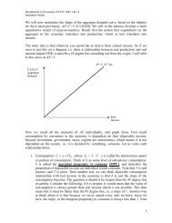
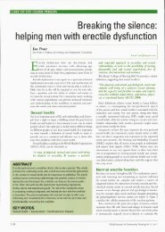

![The Rink - Cyril Dabydeen[1].pdf](https://img.yumpu.com/21946808/1/155x260/the-rink-cyril-dabydeen1pdf.jpg?quality=85)