Multiplier

Introduction to Economics, ECON 100:11 & 13
Multiplier Model
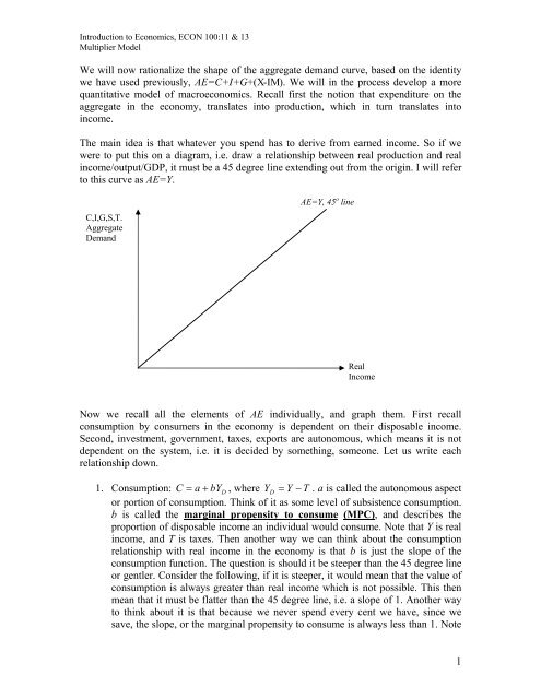
We will now rationalize the shape of the aggregate demand curve, based on the identity
we have used previously, AE=C+I+G+(X-IM). We will in the process develop a more
quantitative model of macroeconomics. Recall first the notion that expenditure on the
aggregate in the economy, translates into production, which in turn translates into
income.
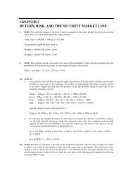
The main idea is that whatever you spend has to derive from earned income. So if we
were to put this on a diagram, i.e. draw a relationship between real production and real
income/output/GDP, it must be a 45 degree line extending out from the origin. I will refer
to this curve as AE=Y.
C,I,G,S,T.
Aggregate
Demand
AE=Y, 45 o line
Real
Income
Now we recall all the elements of AE individually, and graph them. First recall
consumption by consumers in the economy is dependent on their disposable income.
Second, investment, government, taxes, exports are autonomous, which means it is not
dependent on the system, i.e. it is decided by something, someone. Let us write each
relationship down.
1. Consumption: C = a + bY D
, where YD
= Y − T . a is called the autonomous aspect
or portion of consumption. Think of it as some level of subsistence consumption.
b is called the marginal propensity to consume (MPC), and describes the
proportion of disposable income an individual would consume. Note that Y is real
income, and T is taxes. Then another way we can think about the consumption
relationship with real income in the economy is that b is just the slope of the
consumption function. The question is should it be steeper than the 45 degree line
or gentler. Consider the following, if it is steeper, it would mean that the value of
consumption is always greater than real income which is not possible. This then
mean that it must be flatter than the 45 degree line, i.e. a slope of 1. Another way
to think about it is that because we never spend every cent we have, since we
save, the slope, or the marginal propensity to consume is always less than 1. Note
1

Introduction to Economics, ECON 100:11 & 13
Multiplier Model
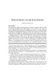
that another way to write the consumption equation in terms of Y and T is
C = a + bY − bT . This means that the greater tax T, the lower the consumption
line. a and b are both positive numbers/constants. Diagramatically,
C,I,G,S,T.
Aggregate
Demand
AE=Y, 45 o line
C = a + bY D
Real
Income
There is also in addition an interesting point. Note that what you do not consume,
you save, which means 1- the marginal propensity to consume give you the
marginal propensity to save.
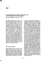
2. Investment, and Government spending are all autonomous. What this means is
that it is a constant at every level of real income. Let the current level be I = I
0
and G = G 0
for investment and government spending respectively.
Diagrammatically, they are just horizontal lines as below.
2

Introduction to Economics, ECON 100:11 & 13
Multiplier Model
C,I,G,S,T.
Aggregate
Demand
AE=Y, 45 o line
I = I 0
G = G 0
Real
Income
3. We lastly examine international trade. Recall that we think of exports as
autonomous. Let the level of export, dependent on our trading partner’s national
income be E = E 0
. However, imports is dependent on our own national income.
Although in our earlier discussion, we have not included an autonomous aspect of
imports, but in general, due to specialization, there is an autonomous aspect to
imports, since an economy cannot produce everything they need. Let the
relationship that describes imports be IM = c + dY . This means that c can be
thought of as autonomous imports, and d as the marginal propensity to import.
Note that the equation says imports are dependent on real income. As in
consumption, necessarily the diagrammatic representation of the line/relationship
must be gentler than the 45 degree line. Note that c and d are both positive
constants and d is a constant that is less than 1. Why? Note that the marginal
propensity to consume (b) plus d cannot be greater than 1. That is because we
know the economy saves, and given that, they cannot consume more than what
they have.
3

Introduction to Economics, ECON 100:11 & 13
Multiplier Model
C,I,G,S,T.
Aggregate
Demand
AE=Y, 45 o line
( c dY )
X − IM = X − +
Real
Income
4. Since we know that aggregate expenditure is the sum of all these above elements
from point 1 to 3. To depict the relationship, all we need is to perform vertical
summation. Why? First, let us sum autonomous G, and I to consumption C.
C,I,G,S,T.
Aggregate
Demand
AE=Y, 45 o line
C + I 0
+ G 0
C + I 0
C
I = I 0
G = G 0
Real
Income
To include net exports, simply do the same. However, note that
X − IM = X − ( c + dY ) is downward sloping with respect to real income, since as
income rises the marginal propensity to import rises. This means that the slope of
the AE line is gentler. What is the slope of the AE curve?
4

Introduction to Economics, ECON 100:11 & 13
Multiplier Model
C,I,G,S,T.
Aggregate
Demand
AE=Y, 45 o line
C + I
0
+ G0
+
C + I 0
+ G 0
( X − IM )
( c dY )
X − IM = X − +
Real
Income
What does the intersection mean? It is of course not possible that aggregate demand not
equating with real income. This means that the point the economy spend, the AE is at the
point at which it intersects with the 45 degree line. Each level of aggregate expenditure is
dependent on the autonomous variables, and the price level. Then as price level rises,
necessarily aggregate expenditure AE falls, while if price level falls, AE rises. How can
we describe this algebraically? At the intersection, AE must equate with real income,
which means:
Y = C + I + G + X − IM
⇒ Y
⇒ Y + dY − bY
⇒ Y
⇒ Y
⇒ Y
= a + bY − bT
( )
a − c − bT0
+ I
0
+ G
=
1+
d − b
1
=
1+
d − b
=
0
+ I
0
+ G
= a − c − bT
0
{ a − c − bT + I + G + X }
0
0
0
+ X
+ I
0
0
+ X
0
0
− c − dY
+ G
0
0
+ X
( autonomous expenditure multiplier) × ( autonomous expenditure)
What does this tell you?
1. An increase(decrease) in autonomous variables, government spending (G),
exports (X), investments (I) would lead to an increase(decrease) in aggregate
expenditure and hence real income.
2. The change in the autonomous variables does not lead to, in general, a $1 for $1
change in real income, and consequently aggregate expenditure. Why? Consider
1
this, if b is greater than d, then 1 + d − b is less than 1, and greater than
1+ d − b
1. When that happens, a $1 increase(decrease) in any of the autonomous variables
listed above (C,I,G) leads to a more than $1 increase(decrease) in aggregate
0
0
5

Introduction to Economics, ECON 100:11 & 13
Multiplier Model
expenditure, and consequently real income. Note that a change in taxes change
aggregate expenditure and hence real income in the opposite direction. This is
what we learned earlier about multiplier effect, and this is the reason why we call
this the multiplier model. What happens when d is greater then b (Consider
an economy with little own production, and hence to rely on imports)? When
would there be no multiplier effect; that is a $1 change lead to a $1 change?
Deriving AD curve
Now we can show how we can use the AE curve to derive the AD curve we learned
earlier. First each AE is given a level of price. A change in prices alters the real income
(the real value of money, and hence how much you can consume and import), however
all the autonomous variables of AE remains unchanged. The diagrammatic relationship is
below,
6

Introduction to Economics, ECON 100:11 & 13
Multiplier Model
C,I,G,S,T.
Aggregate
Demand
AE=Y, 45 o line
AE(P 1 )
AE(P 2 )
AE(P 3 )
Real
Income
/Real
GDP
Price
Level
P 3
P 2
P 1
AD
Real
Output/
Real
GDP
Since each AD is drawn given a level of autonomous expenditures, when those
autonomous expenditures changes, we get a whole new set of AE lines, and consequently
a new AD curve. This explains how AD can be shifted, and allows us to examine how
government policy depending on the type of action shifts the AD and brings about a new
equilibrium in the aggregate economy.
7

Introduction to Economics, ECON 100:11 & 13
Multiplier Model
Limitations of the Model
1. It is not a complete model of the economy. We say this because the model does
not tell us how investments etc are determined within the economy. How do
individuals in the economy really choose how much to consume, and how would
they then react to changes made say by the firms. How do the agents in the
economy determine their expectations?
2. Price level will change in response to changes in AD, which in turn limits the
magnitude of change in real output.
3. Expectations make adjustment process more complicated (Rational Expectations
Model, where agents in the economy are assumed to be rational and uses all
information available to predict the expected equilibrium). What the AD/AS
model and multiplier model does is to say that when the economy is in
disequilibrium (equilibrium away from the long run equilibrium), it either
recovers by itself, or the government does something to bring it back to potential
equilibrium. Consider a negative AD shock that causes a recessionary gap, based
on our argument, the economy either gets back by itself, or does so through direct
spending or other policy. But what if the general outlook in the economy is a
gloomy bearish one. Does government intervention change perception or
expectation of the future? If not, all that will happen may be that the economy
would keep experiencing lower and lower level of C and I, but keeps getting
propped up by government spending with expectations unaltered.
4. Shifts in expenditure may reflect desired shifts in supply and demand (structural
changes) and not just changes by suppliers in response to changes in demand.
Real Business Cycle Theory. What this means then is that by attempting to
adjust the economy on the basis of perceived deviations from the potential output
is incorrect, and disrupts the process of adjustment made within the economy.
Consider a shift in consumption of fuel efficient means of transportation. The
adjustment phase say from gasoline engine vehicles to say methanol vehicles may
induce a huge jump in consumption, pushing the economy out of its potential
output level. But it is simply induced by a real change technology which requires
an adjustment period while everyone readjusts. If the government intervenes
thinking the economy is over heating, say by raising interest rates, it may simply
end up making the change that much tougher. That is the intervention is totally
superfluous, because once all the changes runs itself out, the economy would get
back to its potentially level. Real Business Cycle Theory highlights that
fluctuations in the economy is a reflection of real changes in the economy (such
as the technology change requiring adjustment time), so that it is a simultaneous
change in demand and supply, and not just to reactions by supply from changing
demand.
Expenditures in the model thus far say that changes in current income, changes
consumption. However, do individuals really do that, or do they base their consumption
on lifetime income? Consider the following, when you choose to attend university, did
you do you based on your current income or future lifetime income. In general, an
individual’s consumption is partially based on what they foresee their income would be
in long run, and current income. That is there is a portion of the individual’s income she
is always willing to use regardless of his current income. Then changes to current income
8

Introduction to Economics, ECON 100:11 & 13
Multiplier Model
will not affect her spending/consumption habits. But of course it is more common that if
the deviation is quite substantial, such as a lottery winning, we would expect here to raise
current consumption quite a bit immediately. This idea is know as the Permanent
Income Hypothesis which says that expenditures are based on permanent of lifetime
income, and not transitory changes in income. When this happens the MPC out of current
income is zero, and the multiplier is 1, ignoring the effect out of importing.
9