Solving Stochastic Differential Equations with Maple
Solving Stochastic Differential Equations with Maple
Solving Stochastic Differential Equations with Maple
Create successful ePaper yourself
Turn your PDF publications into a flip-book with our unique Google optimized e-Paper software.
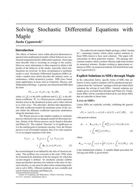
<strong>Solving</strong> <strong>Stochastic</strong> <strong>Differential</strong> <strong>Equations</strong> <strong>with</strong><br />
<strong>Maple</strong><br />
Sasha Cyganowski<br />
Introduction<br />
The effects of intrinsic noise <strong>with</strong>in physical phenomena is<br />
ignored when mathematical models of their behavior are constructed<br />
using deterministic differential equations. Such equations<br />
describe what is occurring on average to the system.<br />
However, more information is often required to obtain a full<br />
picture of the behavior of the model, especially when nonlinearities<br />
are involved. In these circumstances a stochastic<br />
model is used. <strong>Stochastic</strong> <strong>Differential</strong> <strong>Equations</strong> (SDEs) include<br />
a random term which describes the intrinsic noise, or<br />
randomness, <strong>with</strong>in dynamical systems. SDEs have found<br />
many applications in areas such as Chemistry, Physics, and<br />
Mathematical Biology. A general, one-dimensional SDE takes<br />
the form<br />
dX t = a(t; X t)dt + b(t; X t)dW t; (1)<br />
where a(t; X t) is the drift coefficient and b(t; X t) is the diffusion<br />
coefficient. W t is a Wiener process which represents<br />
intrinsic noise in the dynamical system, and is often referred<br />
to as white noise. The subscript t denotes time-dependence.<br />
The drift coefficient models the dominant action of the system<br />
whilst the diffusion coefficient represents randomness<br />
along the dominant curve.<br />
The Wiener process is the simplest random or stochastic<br />
process which provides an adequate model for Brownian motion.<br />
Details of the Wiener process can be found in Kloeden<br />
and Platen [3]. This random “function” is of significance as<br />
it is the starting point of stochastic calculus. Now, the Wiener<br />
process is not of bounded variation, thus if we write equation<br />
(1) as an integral equation of the form<br />
Xt(w) = Xt0 (w) +<br />
+<br />
Z t<br />
t0<br />
Z t<br />
t0<br />
a[s; X s(w)] ds<br />
b[s; X s(w)] dW s(w); (2)<br />
the second integral is not defined by the rules of classical calculus.<br />
This problem was overcome in the early 1950s when<br />
Ito formulated his definition of the Ito integral, for which the<br />
second integral is defined. Ito stochastic calculus exhibits<br />
many peculiarities and does not conform to the rules of classical<br />
calculus, so care must be taken when constructing methods<br />
to solve SDEs. Efficient methods are now available and<br />
can be found in Kloeden and Platen [3].<br />
School of Computing and Mathematics, Deakin University, Geelong,<br />
Vic 3217, Australia. sash@deakin.edu.au<br />
The author has developed a <strong>Maple</strong> package, called “stochastic”,<br />
containing routines which return explicit solutions to<br />
those SDEs known to have such solutions. This paper will<br />
concentrate on these particular routines. The package also<br />
contains routines which construct efficient, high order stochastic<br />
numerical schemes. Readers wishing to approximate solutions<br />
to SDEs via numerical methods will benefit from reading<br />
Cyganowski [1].<br />
Explicit Solutions to SDEs through <strong>Maple</strong><br />
In the subsections below, specific forms of SDEs that are<br />
known to have explicit solutions will be introduced and procedures<br />
from the “stochastic” package will be provided which<br />
automate the solving of such SDEs. General solutions are<br />
simply given, as found from Kloeden and Platen [3]. Firstly,<br />
linear SDEs will be considered followed by non-linear SDEs<br />
that are reducible to linear form.<br />
LINEAR SDES<br />
Linear SDEs are explicitly solvable, exhibiting the general<br />
form<br />
dX t =(a(t)X t + c(t))dt +(b(t)X t + d(t))dW t; (3)<br />
<strong>with</strong> general solution<br />
where<br />
X t = t;t0 (X t0 +<br />
t;t0<br />
+<br />
= exp(<br />
Z t<br />
t0<br />
Z t<br />
t0<br />
Z t<br />
t0<br />
,1<br />
s;t0<br />
(c(s) , b(s)d(s)) ds<br />
,1<br />
s;t0 d(s) dW s); (4)<br />
(a(s) , 1<br />
2 b2 (s)) ds +<br />
Z t<br />
t0<br />
b(s) dW s) (5)<br />
is the fundamental solution. A suitable <strong>Maple</strong> procedure for<br />
solving such SDEs is given below.<br />
1
<strong>Stochastic</strong> DEs <strong>with</strong> <strong>Maple</strong><br />
> linear:=proc(a:algebraic,b:algebraic)<br />
> local temp1,alpha,beta,gamma,delta,fundsoln,<br />
> fundsoln2,soln,default1,default2,default3;<br />
> if diff(a,x,x) 0<br />
> or diff(b,x,x) 0 then<br />
> ERROR(`SDE not linear, try a reducible<br />
> procedure`)<br />
> else<br />
> alpha := diff(a,x);<br />
> alpha := subs(t = s,alpha);<br />
> beta := diff(b,x);<br />
> beta := subs(t = s,beta);<br />
> if diff(beta,s) = 0 then<br />
> temp1 := beta*W;<br />
> else temp1 := Int(beta,W = 0 .. t);<br />
> fi;<br />
> gamma := coeff(a,x,0);<br />
> gamma := subs(t = s,gamma);<br />
> delta := coeff(b,x,0);<br />
> delta := subs(t = s,delta);<br />
> fundsoln := exp(int(alpha-1/2*(beta**2),<br />
> s = 0 .. t)+temp1);<br />
> fundsoln2 := subs(t = s,fundsoln);<br />
> if beta = 0 then<br />
> soln := fundsoln*(X[0]+<br />
> int(1/fundsoln2*<br />
> (gamma-beta*delta),s = 0 .. t)<br />
> +Int(1/fundsoln2*delta,W = 0 .. t))<br />
> else soln := fundsoln*(X[0]+<br />
> Int(1/fundsoln2*<br />
> (gamma-beta*delta),s = 0 .. t)<br />
> +Int(1/fundsoln2*delta,W = 0 .. t))<br />
> fi;<br />
> default1 := Int(0,W = 0 .. t) = 0;<br />
> default2 := Int(0,W = 0 .. s) = 0;<br />
> default3 := Int(0,s = 0 .. t) = 0;<br />
> soln := X[t] = subs(default1,default2,<br />
> default3,soln)<br />
> fi<br />
> end:<br />
To invoke such a procedure we use the following command.<br />
linear(a(t,x),b(t,x));<br />
Figure 1 Syntax for procedure “linear”.<br />
In Figure 1, a(t; x) and b(t; x) denote the drift and diffusion<br />
coefficients of the SDE, respectively. Note that both arguments<br />
must be given in the variables x and t. This syntax<br />
will be required for all the procedures in this paper.<br />
REDUCIBLE SDES<br />
SDEs are in this category if they have the general form<br />
dX t =( b(X t)h + 1<br />
<strong>with</strong> general solution<br />
2<br />
X t = h ,1 (exp t h(X0) + exp t<br />
2 b(X t)b 0 (X t))dt + b(X t)dW t; (6)<br />
Z t<br />
0<br />
exp , s dW s); (7)<br />
where<br />
h =<br />
Z x ds<br />
b(s)<br />
: (8)<br />
A suitable <strong>Maple</strong> procedure for solving such SDEs is given<br />
below.<br />
> reducible:=proc(a:algebraic,b:algebraic)<br />
> local beta,temp1,h,alpha,soln,soln1;<br />
> h := int(1/b,x);<br />
> temp1 := alpha*b*h+1/2*b*<br />
> simplify(diff(b,x));<br />
> temp1 = a;<br />
> alpha := simplify(solve(",alpha));<br />
> beta := alpha*h;<br />
> if diff(alpha,x) = 0 then<br />
> if alpha=0 then<br />
> soln:=h=subs(x=X[0],h)+W;<br />
> X[t]=simplify(solve(soln,x));<br />
> else<br />
> soln1 := h = exp(alpha*t)*<br />
> subs(x = X[0],h)<br />
> +exp(alpha*t)*Int(exp(-alpha*s),<br />
> W = 0 .. t);<br />
> X[t] = solve(soln1,x);<br />
> fi<br />
> elif diff(beta,x) = 0 then<br />
> X[t] = simplify(solve(h=beta*t+W+<br />
> subs(x=X[0],h),x));<br />
> else ERROR(`non-linear SDE not reducible`)<br />
> fi<br />
> end:<br />
GENERAL MAPLE PROCEDURE FOR FINDING<br />
EXPLICIT SOLUTIONS.<br />
The <strong>Maple</strong> procedure “explicit” is given below, which is a<br />
combination of procedures “linear” and “reducible”. This<br />
procedure determines whether an SDE is reducible or linear,<br />
and solves it accordingly. If the SDE does not fall into one<br />
of the above categories, the user is returned <strong>with</strong> an error<br />
message.<br />
> explicit:=proc(a:algebraic,b:algebraic)<br />
> if diff(a,x,x) = 0 and diff(b,x,x) = 0 then<br />
> linear(a,b)<br />
> else<br />
> reducible(a,b)<br />
> fi<br />
> end:<br />
The procedure “explicit” is more user-friendly than “linear”<br />
or “reducible” as it is not necessary for the user to predetermine<br />
which category the SDE belongs to.<br />
Applications<br />
(I) Consider the SDE<br />
dX t = dt +2<br />
p XtdW t: (9)<br />
Here we see how the procedure “explicit” can be used to find<br />
the explicit solution of equation (9).
explicit(1,2*sqrt(x));<br />
X t =2<br />
(II) Consider the SDE<br />
p X0W + W 2 + X0<br />
dX t =lnX tdt + X tdW t: (10)<br />
In this example the SDE is reported to have no known<br />
explicit solution.<br />
> explicit(ln(x),x);<br />
Error, (in reducible) non-linear SDE not reducible<br />
Conclusion<br />
<strong>Stochastic</strong> calculus has been introduced in this paper through<br />
the computer algebra system <strong>Maple</strong>. Procedures were presented<br />
and used to find solutions to SDEs. It should be noted<br />
that the methods provided here for solving SDEs are suitable<br />
for real-valued, one-dimensional SDEs <strong>with</strong> real-valued,<br />
one-dimensional Wiener processes.<br />
Symbolic computation in stochastic analysis has been investigated<br />
by Kendall [2] and Valkeila [6], while <strong>Maple</strong> code<br />
suitable for use in stochastic numerics has been developed<br />
by Cyganowski [1] and Kloeden and Scott [5]. Previously<br />
<strong>Maple</strong> had not been used in stochastic calculus for finding<br />
explicit solutions to SDEs.<br />
The procedures in this paper are part of the <strong>Maple</strong> package<br />
“stochastic” which has been developed by the author<br />
and recently accepted into <strong>Maple</strong>'s share library. It will become<br />
publicly available when the next electronic update of<br />
the share library occurs. Those who are interested in acquiring<br />
the package now are welcome to contact the author for<br />
a free copy, complete <strong>with</strong> help files and installation instructions.<br />
Alternatively, the package can be obtained via the Internet<br />
at http://www.cm.deakin.edu.au/~sash/maple.html.<br />
Other functions contained in the “stochastic” package include<br />
procedures which construct strong stochastic numerical<br />
schemes up to order 2, weak stochastic numerical schemes<br />
up to order 3, as well as procedures which check for commutative<br />
noise of the first and second kind, and a procedure<br />
which converts SDEs <strong>with</strong> white noise into colored noise<br />
form. Additional procedures are included <strong>with</strong>in the package<br />
so that users can easily construct numerical schemes other<br />
than those already available.<br />
Future extensions to this package will include a set of<br />
procedures which plot approximate solutions to SDEs. The<br />
input required for these “graphical” procedures will be easily<br />
obtainable as it will be the output from the “algebraic”<br />
procedures discussed in this paper.<br />
References<br />
<strong>Stochastic</strong> DEs <strong>with</strong> <strong>Maple</strong><br />
[1] Cyganowski, S.O., A MAPLE Package for <strong>Stochastic</strong><br />
<strong>Differential</strong> <strong>Equations</strong>, Computational Techniques<br />
and Applications: CTAC95, editors A. Easton, R. May,<br />
World Scientific, (to appear).<br />
[2] Kendall, W.S., Computer algebra and stochastic calculus,<br />
Notices Amer. Math. Soc., 37, 1990, 1254–1256.<br />
[3] Kloeden, P.E. and Platen, E., Numerical Solution<br />
of <strong>Stochastic</strong> <strong>Differential</strong> <strong>Equations</strong>, Springer-Verlag,<br />
1992.<br />
[4] Kloeden, P.E., Platen, E. and Schurz, H., Numerical Solution<br />
of <strong>Stochastic</strong> <strong>Differential</strong> <strong>Equations</strong> through Computer<br />
Experiments, Springer-Verlag, 1993.<br />
[5] Kloeden, P.E. and Scott, W.D., Construction of <strong>Stochastic</strong><br />
Numerical Schemes through <strong>Maple</strong>, <strong>Maple</strong> Technical<br />
Newsletter, 10, 1993, 60–65.<br />
[6] Valkeila, E., Computer algebra and stochastic analysis,<br />
some possibilities, CWI Quarterly, 4, 1991, 229–238.<br />
3


