Assessing Uncertainty in Future Pressure Changes Predicted By ...

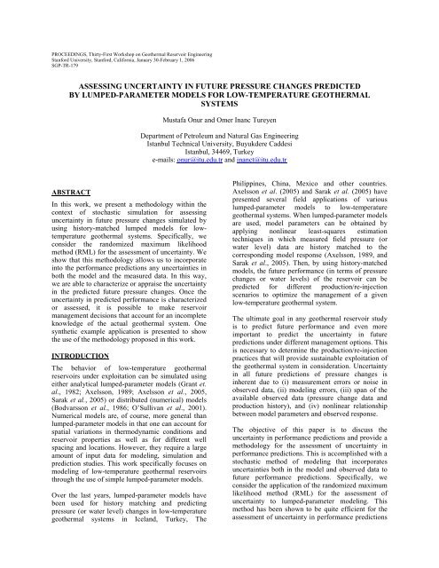
PROCEEDINGS, Thirty-First Workshop on Geothermal Reservoir Engineering
Stanford University, Stanford, California, January 30-February 1, 2006
SGP-TR-179
ASSESSING UNCERTAINTY IN FUTURE PRESSURE CHANGES PREDICTED
BY LUMPED-PARAMETER MODELS FOR LOW-TEMPERATURE GEOTHERMAL
SYSTEMS
ABSTRACT
In this work, we present a methodology within the
context of stochastic simulation for assessing
uncertainty in future pressure changes simulated by
using history-matched lumped models for lowtemperature
geothermal systems. Specifically, we
consider the randomized maximum likelihood
method (RML) for the assessment of uncertainty. We
show that this methodology allows us to incorporate
into the performance predictions any uncertainties in
both the model and the measured data. In this way,
we are able to characterize or appraise the uncertainty
in the predicted future pressure changes. Once the
uncertainty in predicted performance is characterized
or assessed, it is possible to make reservoir
management decisions that account for an incomplete
knowledge of the actual geothermal system. One
synthetic example application is presented to show
the use of the methodology proposed in this work.
INTRODUCTION
The behavior of low-temperature geothermal
reservoirs under exploitation can be simulated using
either analytical lumped-parameter models (Grant et.
al., 1982; Axelsson, 1989; Axelsson et al., 2005,
Sarak et al., 2005) or distributed (numerical) models
(Bodvarsson et al., 1986; O’Sullivan et al., 2001).
Numerical models are, of course, more general than
lumped-parameter models in that one can account for
spatial variations in thermodynamic conditions and
reservoir properties as well as for different well
spacing and locations. However, they require a large
amount of input data for modeling, simulation and
prediction studies. This work specifically focuses on
modeling of low-temperature geothermal reservoirs
through the use of simple lumped-parameter models.
Over the last years, lumped-parameter models have
been used for history matching and predicting
pressure (or water level) changes in low-temperature
geothermal systems in Iceland, Turkey, The
Mustafa Onur and Omer Inanc Tureyen
Department of Petroleum and Natural Gas Engineering
Istanbul Technical University, Buyukdere Caddesi
Istanbul, 34469, Turkey
e-mails: onur@itu.edu.tr and inanct@itu.edu.tr
Philippines, China, Mexico and other countries.
Axelsson et al. (2005) and Sarak et al. (2005) have
presented several field applications of various
lumped-parameter models to low-temperature
geothermal systems. When lumped-parameter models
are used, model parameters can be obtained by
applying nonlinear least-squares estimation
techniques in which measured field pressure (or
water level) data are history matched to the
corresponding model response (Axelsson, 1989, and
Sarak et al., 2005). Then, by using history-matched
models, the future performance (in terms of pressure
changes or water levels) of the reservoir can be
predicted for different production/re-injection
scenarios to optimize the management of a given
low-temperature geothermal system.
The ultimate goal in any geothermal reservoir study
is to predict future performance and even more
important to predict the uncertainty in future
predictions under different management options. This
is necessary to determine the production/re-injection
practices that will provide sustainable exploitation of
the geothermal system in consideration. Uncertainty
in all future predictions of pressure changes is
inherent due to (i) measurement errors or noise in
observed data, (ii) modeling errors, (iii) span of the
available observed data (pressure change data and
production history), and (iv) nonlinear relationship
between model parameters and observed response.
The objective of this paper is to discuss the
uncertainty in performance predictions and provide a
methodology for the assessment of uncertainty in
performance predictions. This is accomplished with a
stochastic method of modeling that incorporates
uncertainties both in the model and observed data to
future performance predictions. Specifically, we
consider the application of the randomized maximum
likelihood method (RML) for the assessment of
uncertainty to lumped-parameter modeling. This
method has been shown to be quite efficient for the
assessment of uncertainty in performance predictions

for nonlinear problems (Kitanidis et al., 1995; Oliver
et al., 1996; Liu and Oliver, 2003; Gao et al., 2005).
The paper begins with a brief review of lumpedparameter
models considered in this study. Then,
history matching and performance prediction
problems within the context of maximum likelihood
and randomized maximum likelihood methods are
discussed. Finally, a synthetic example application is
presented to demonstrate the methodology proposed
in this study for the assessment of uncertainty in
performance predictions by lumped-models for lowtemperature
geothermal systems.
LUMPED PARAMETER MODELING
The lumped-parameter modeling considered here is
very similar in concept to the one presented
originally by Axelsson (1989) and identical to the
one presented later by Sarak et al. (2003a, 2003b, and
2005). As in these works, our lumped-parameter
models are based on the conservation of mass only
and hence are valid for low-temperature liquid
reservoirs under the assumption that variations in
temperature within the system can be neglected (i.e.
the simulated systems are assumed to be isothermal).
Lumped-parameter modeling can be regarded as a
highly simplified form of numerical modeling. In
numerical models, a geothermal system is
represented by many (>100 to 10 6 ) gridblocks. On the
other hand, in lumped-parameter modeling, a
geothermal system is represented by only a few
homogeneous tanks and is visualized as consisting of
mainly three parts: (1) the central part of the
reservoir; (2) outer parts of the reservoir, and (3) the
recharge source. The first two are treated as series of
homogeneous tanks with average properties. The
recharge (or constant pressure) source can be
connected to the other parts of the reservoir or
directly to the central part of the reservoir and is
treated as a “point source” that recharges the system.
If there is no connection to the recharge source, the
model would be closed, otherwise would be open.
Two different open lumped-parameter models are
depicted in Fig. 1.
Recharge
source (pi)
αo1
Outer part
κo1
αr
Reservoir
κr
Net
production
(a) two-tank open lumped-parameter model
Recharge
source (pi)
Outer part 2
Outer part 1
κo2
κo1
αo2 αr
αo1
Net
production
Reservoir
κr
(b) three-tank open lumped-parameter model
Figure 1. Two different lumped-parameter models.
The model shown in Fig. 1(a) represents a two-tank
open lumped model, where the first tank, in which
production/injection occurs, represents the innermost
(or central) part of the geothermal system. The
changes in pressure in this part are monitored and
production/injection rates are recorded. In the second
tank, representing the outer part of the reservoir that
is connected to the recharge source, there is neither
production nor injection, and it recharges the central
reservoir. Fluid production causes the pressure in the
reservoir to decline, which results in water influx
from the outer to the central part of the reservoir. The
recharge source represents the outermost part of the
geothermal system.
When using the lumped-parameter models considered
in this work (Fig. 1), the simulated model (output)
response represents pressure or water level changes
for an observation well for a given net production
history (input). The number of model parameters
increases as the number of tanks or the complexity of
the lumped model increases.
Here and throughout, α represents the recharge
constant between the tanks in kg/(bar-s), κ represents
the storage capacity (or coefficient) of a tank in
kg/bar, and pi represents the initial pressure of the
recharge source in bar. The geothermal system is
assumed to be in hydrodynamic equilibrium initially;
i.e., the initial pressure, pi, is uniform in the system.
In cases for which the initial system pressure (or
initial water level), pi, is known, pi can be eliminated
from the unknown set of model parameter vector.
Further details about the lumped-parameter models
used in this study can be found in Sarak et al. (2003a,
b, and 2005).
HISTORY-MATCHING PROBLEM
After a period of production from a geothermal
reservoir, and based on the production/injection rate
history given, a lumped-parameter model can be
matched to the observed pressure (or water level)
data to obtain the parameters of that particular model.
Here and throughout, obs
y refers to the vector of
measured or observed pressure change data, and
contains all Nd pressure change measurements that
will be used for estimating the model parameters by

nonlinear regression. We let CD be the NdxNd
symmetric positive-definite covariance matrix for
pressure change measurement errors, and assume that
measurement errors for pressure data are Gaussian
with mean zero (vector) and covariance matrix CD
[i.e., N(0, CD)]. N(0, CD) represents a normal
distribution with mean zero and covariance matrix
CD. Throughout, a boldface capital letter denotes a
matrix, while a boldface lower case letter denotes a
column vector.
Letting e denote the Nd-dimensional vector of errors
for observed data and ( 1, 2,
, ) T
m = m m L mM
denote the
vector of unknown model parameters that are
estimated, it follows that
y = f( m) + e. (1)
obs
Here f refers to the Nd-dimensional vector of
computed pressure-change data from a considered
lumped model, for a given m . M represents the total
number of unknown model parameters.
As noted above, e is N(0, CD). Thus, the likelihood
function for the model conditional to observed data is
given by (Bard, 1974)
1
T
⎧ −1
⎫
L(
myobs ) ∝exp ⎨− [ yobs − fm ( ) ] CD[ yobs − fm ( ) ] ⎬
⎩ 2
⎭
(2)
where the superscripts “T” and “-1” represent
transpose of a vector and inverse of a matrix,
respectively. The maximum likelihood estimate of m,
which honors measured pressure data, is obtained by
maximizing Eq. 2, or equivalently, minimizing the
objective function O(m) given by
T
obs D obs
−1
[ ] [ ]
O(
m) = y − f( m) C y − f( m ) . (3)
Eq. 3 is the objective function for the well known
general nonlinear least-squares method, and assumes
that the data error covariance matrix CD is known.
Often we do not have enough information to
construct the data error covariance matrix CD that
may account correlation between measurement
errors. Hence, the commonly used assumption is that
the Nd × Nd
CD is a diagonal matrix in Eq. 3. If data
measurement errors are independent random
2
variables with mean zero and known variance σ
d, j
for each observed data yobs,j, then CD is a diagonal
2
matrix with diagonal entries equal to σ d, j,
j=1,2,…,Nd. In this case, Eq. 3 reduces to the well
known weighted least-squares objective function:
( m)
Nd
⎡ yobs, j − f ⎤ j
O(
m ) = ∑ ⎢ ⎥ . (4)
j = 1 ⎢⎣ σd,
j ⎥⎦
If we further assume that error variances 2
σ d, jare
2 2
identical, i.e., σ = σ for all j, then Eq. 4 with
d , j d
2 1/( σ d ) deleted defines the objective function for the
un-weighted (ordinary) least-squares procedure.
The lumped-parameter model responses are nonlinear
with respect to the model parameters. Thus, Eq. 3 (or
4) calls for nonlinear minimization techniques. Over
the past, we have found that the gradient based
algorithms such as the Levenberg-Marquardt method
based on a restricted procedure described by Fletcher
(1987) is quite efficient to minimize Eq. 3 or 4.
It is important to note that within the context of
maximum likelihood estimation, the observed data
yobs would represent a single realization of the
observed data from a normal distribution with mean
zero and known covariance matrix, CD, and thus the
model vector m is considered as a random variable
because different realizations of yobs would provide
different estimates of m. Thus, when historymatching
problem is viewed within the context of the
principle of maximum likelihood estimation, one can
attach statistical measures to quantify the quality of a
match as well as the uncertainty of the model
parameters estimated. The standard statistical
measures used for assessing the quality of a match
and the reliability of estimated parameters are the
root-mean-square error (RMS) and confidence
(usually 95% percent) intervals.
The value of RMS defined by Eq. 5 shows the quality
of fit quantitatively.
Nd
1
RMS = y − f
N
2
∗ ( )
2
∑ ⎡
obs, j j m ⎤ , (5)
⎣ ⎦
d i=
1
∗
where m represents the optimized parameter vector.
The lower the RMS value, the better the fit between
field and computed data. As we will discuss later, this
does not necessarily mean that the lumped-model
giving the smallest RMS value be the most
appropriate model for the history-matched data and
should give the most reliable predictions.
While it is important to improve the overall match of
available data, it is equally or even more important
that the history-matched model be able to predict
reliably the uncertainty (from a statistical point of
view) in predictions due to the fact that a certain
amount of error (i.e., modeling and measurement
errors, etc) will always be introduced into the

estimated parameters from the history-matching
process. In history matching, increasing complexity
of the lumped-model (or equivalently increasing the
number of tank and hence the model parameters) may
improve the overall fitting of the model to the current
data at the expense of destroying and ignoring the
underlying statistical basis for nonlinear least-squares
parameter estimation based on the principle of
maximum likelihood.
Statistical confidence intervals are known as a useful
tool to give a quantitative evaluation of model
discrimination and assessment of uncertainty in the
estimated parameters (Dogru et al., 1977; Anraku and
Horne, 1995). From the least-squares theory under
the assumption that a nonlinear model can be
∗
linearized around the optimal estimate m , we know
that confidence intervals contain information about
both the statistical standard deviation (s, see Eq. 7) of
the match (related to the RMS value) and the
sensitivity of observed data to the parameters. In
general, the larger the confidence interval, the higher
the uncertainty in the estimated model parameters.
The γ × 100% approximate confidence intervals are
computed from (Bard, 1974; Dogru et al. 1977)
)
m −t( 1 −γ/2, N −M) s ⎡( G C G ) ⎤ ≤m
, (6)
∗
i d ⎣
T
∗
m
−1 D ∗
m
−1
⎦ii
i
∗
≤ mi + t( 1 −γ/2, Nd −M)
s
T −1 −1
⎡( ∗ D ∗ ⎣
G C G ) ⎤
m m ⎦ ii
∗ where m denotes the estimate obtained by
minimizing O (Eq. 3), i
m∗ denotes the estimate of i th
model parameter at the minimum, G ∗ denotes the
m
Nd × M sensitivity matrix (containing derivatives of
observed data with respect to model parameters)
∗
evaluated at the estimate m , i m) represents the true,
but unknown value of the model parameter, mi, and
t(1 −γ/ 2, N − M)
is the value that cuts off
d
(1 − γ ) / 2× 100% in the upper tail of t-distribution
with Nd − M degrees of freedom. (Taking γ = 0.95 in
Eq. 6 gives %95 percent confidence intervals.) In Eq.
6, s is computed from
s =
∗
O(
m )
. (7)
N − M
d
It may be worth noting that s computed from Eq. 7 is
a dimensionless quantity. If the quantity s is
significantly greater than unity, this indicates either
that the lumped-model is inappropriate to reproduce
the pressure data, or that the magnitude of the
pressure measurement errors reflected by the
covariance matrix CD is underestimated. If the model
is correct, and s computed from Eq. 7 is significantly
larger than 1, this indicates that the covariance matrix
CD used in Eq. 3 underestimates the true, but
unknown covariance matrix CD. If the model used for
observed data is correct, and we use the correct error
covariance matrix, then we should expect s to be
close to unity.
We should perhaps dedicate a few words to the
philosophy underlying the use of RMS and
confidence intervals to discriminate the best fitting
model among the candidate lumped models selected
for history matching. There is a relationship between
the confidence intervals and the RMS. This
relationship could be complicated in the models
having large number of model parameters and when
the parameters show correlation among them. One
may expect the uncertainty as reflected by the
confidence intervals for some parameter estimates to
increase with the increasing complexity of a model,
while the value of RMS (or equivalently the quality
of a fit as defined by Eq. 7) improves. However, in
our view, as long as the lumped model selected is
appropriate and there are sufficient observed data
available to support the model, all parameters should
have “acceptable” confidence interval ranges and the
RMS value should be close to the standard deviation
of measurement errors in observed pressure data.
Then, one can accept the model. Otherwise, one
rejects the model because confidence intervals do not
support the model from a statistical point of view. In
short, in our view, the best fitting lumped model is
the one providing not only the smallest possible
acceptable confidence intervals for all parameters but
also the smallest possible RMS value among the
lumped-models used for history matching. Here, our
definition is that an estimate of a parameter is
acceptable if its confidence interval range is less than
95% of the estimated value itself. As also shown later
by a synthetic example application, it is important to
compute the confidence intervals for the parameters
in addition to the RMS (or the value of s given by Eq.
7). The application of this same methodology to a
few field examples has also been demonstrated by
Sarak et al. (2005).
PREDICTION OF FUTURE PERFORMANCE
The most important objective of lumped-parameter
modeling is to predict future responses to given
production scenario. The parameter estimation (or
history-matching) procedure provides values of the
model parameters to be inserted into the prediction
model equations. Although forecasting future
performance is similar to parameter estimation in that
they both involve the history matching of measured
data, in performance prediction we have also to
tackle the element of uncertainty in the model
parameters and in the data observations, caused by
measurement errors. First we discuss the linear leastsquares
theory, and then the more general nonlinear

case how to characterize the uncertainty in future
predicted response.
Assuming that a nonlinear model can be linearized
around the optimum parameter vector and that the
measurement errors on the observed past and future
data to be observed are independent, identically
distributed random variables with mean zero and
2 variance σ d (i.e., CD in Eq. 3 is a diagonal matrix
2 2 2
with all diagonal entries equal to σ d or σd, i = σ d in
Eq. 4), we can show that the variance of the predicted
value of y pi , at a given time ti such that ti > tN
is
d
given by (Bard, 1974; Dogru et al., 1977; Sen and
Srivastava, 1990)
( ) 1 −
−
σ σ g G ∗C G ∗ g . (8)
2 2 2 T T 1
p, i = d + s i m D m i
Here, gi is the M-dimensional sensitivity vector of
predicted response at any time ti:
T ⎡∂y ∂y ∂y
⎤
g i = ⎢ ⎥ , (9)
p, i p, i p, i
, , K,
⎣ ∂m1 ∂m2 ∂mM⎦
where each sensitivity is evaluated at the optimized
∗
parameter vector, m obtained from history matching
−
∗
m D ∗
m
G C G is the M × M approximate
period. ( ) 1
T −1
∗
Hessian matrix evaluated at m and also represents
∗
the covariance matrix of the estimated m . The
diagonal entries of this matrix represent the variances
of model parameters, while its off diagonal entries
represent the covariances (or correlations) between
the two model parameters. This matrix does not vary
with the prediction time ti because it is determined
from the history-matching period by minimizing Eq.
2
3. If σ d is not known, it can be estimated from the
history-matching period:
σ
∗ ( m )
Nd
∑ ⎡yobs, i − f ⎤
⎣ i ⎦
2 i=
1
d =
Nd−M . (10)
2
As is clear from Eq. 8, the uncertainty (or σ pi , ) in the
predicted response is controlled by the variance and
covariance of the estimated parameters through the
matrix ( ) 1 −
T −1
G ∗CDG ∗ and the quality of fit s m m
2
computed from history matching period as well as the
sensitivity of the predicted response to the estimated
model parameters through the vector g i computed in
2
the prediction period. In general, the behavior of σ pi ,
can be quite complicated depending on the
magnitudes of
and ( ) 1 −
T T −1
2
σ d (or the quality of match, s 2 )
giG ∗CDG ∗ g m m i . However, theoretically, we
would expect that as the complexity of the model
increases, the magnitude of s 2 2
(or the variance σ d in
the case where it is unknown and estimated from Eq.
10) decreases, while that of ( ) 1 −
T T −1
giG ∗CDG ∗ g
m m i
increases. We usually expect that the behavior of the
predicted response is more controlled by the
magnitude of ( ) 1 −
T T −1
giG ∗CDG ∗ g m m i than that of s 2 for
the lumped models. In fact, as shown later, our
results show that when an over parameterized model
instead of the correct lumped model is used for
history matching, the uncertainty in predicted
performance is overestimated, while using a less
parameterized model provides an underestimated
variance in the predicted response. Approximate
confidence limits based on Eq. 8 for the predicted
responses can be also constructed (Dogru et al.,
1977; Sen and Srivastava, 1990). These limits can
characterize the uncertainty in future predicted
responses.
As mentioned above, Eq. 8 is based on linearization
of the predicted response around the optimal
parameter vector. Hence, Eq. 8 may not provide a
reliable estimate of the uncertainty on the predicted
response if the linearization is not valid.
For nonlinear problems, it has been shown that
although it is approximate, the randomized maximum
likelihood method (RML) does a good job for
assessing the uncertainty in the predicted response
(Kitanidis et al., 1995; Oliver et al., 1996; Liu and
Oliver, 2003; Gao et al., 2005). By these authors, the
RML has been considered within the Bayesian
estimation framework for under-determined problems
(i.e., the unknown model parameters far exceeds the
number of observed data, M > Nd) with a prior model
for the parameters. Here, we apply the RML method
for the lumped-parameter modeling without a prior
model, which usually constitutes an over-determined
problem (Nd >> M). In this case, the RML would
provide sampling of the likelihood probability
density function for the model conditional to
observed data, given by (Bard, 1974)
⎧ 1 ⎫
p( myobs ) = cexp⎨− O(
m ) ⎬
(11)
⎩ 2 ⎭
where O(m) is given by Eq. 1 and c is a normalizing
constant.
In the RML sampling procedure of Eq. 11, a
conditional realization of the model parameters to
observed data can be generated as follows: (i)

provide an initial guess of the model parameter
vector m, (ii) add noise to the observed data (i.e., a
1/2
realization of observed data) by yuc= yobs + CDz u ,
where zu is an Nd-dimensional vector of independent
standard random normal deviates. In the applications
considered in this paper, 1/2
CD is a diagonal matrix
with entries equal to the square roots of the
corresponding diagonal entries of CD; (iii) generate a
conditional realization of the model parameter vector
*
m r by minimizing Eq. 1 with yobs replaced by yuc;
(iv) check to see if the estimated model parameter
*
vector m r gives an acceptable match of the data.
*
This is done based on the assumption that if m r is a
legitimate realization of Eq. 11, then it should satisfy:
2 *
2
1−5 ≤ON( m r)
≤ 1+ 5
(12)
N −M N −M
d d
N mr m r d is the
normalized objective function. Eq. 12 is obtained
from the fact that O ( r )
*
m is a chi-squared (χ 2 )
distribution with mean Nd-M and variance 2(Nd-M)
(Barlow, 1989; Gao et al. 2005). In Eq. 12, it is
assumed that the realization should be within five
standard deviations. If the realization *
m r does not
satisfy Eq. 12, then it may mean that the nonlinear
minimization of Eq. 1 has resulted in a local
minimum or that the noise level in observed data has
been underestimated/overestimated or the model is
not appropriate (Gao et al., 2005). To generate n
conditional realizations, we repeat the procedure
described by items (i) through (iv) n times. After n
acceptable realizations of the model parameter
*
vector, m r , for r=1,2,…,n, are generated, we can
predict n realizations of the future response using
*
these n m r realizations in the lumped-parameter
model considered for a given future production
scenario. Then, we can characterize the uncertainty in
the predicted response by constructing the histogram
and/or cumulative frequency based on these n
realizations of the predicted responses at any given
prediction time ti such that t > t .
* *
where O ( ) = O( )/2(
N −M)
EXAMPLE APPLICATION
i Nd
Here, we consider one synthetic example application
to demonstrate the application of the methodology
proposed in this work.
Suppose that our true model for the geothermal
system is a two-tank open lumped-parameter model
as shown in Fig. 1(a). The true pressure change and
net production history data for a twenty-year period
are shown in Fig. 2. (Note that pressure change is
initial pressure minus the reservoir pressure, and thus
as reservoir pressure decreases with production,
pressure change increases.) The true input model
parameters are shown in the second column of Table
1.
Table 1. Estimated model parameters by historymatching
of observed data with three
different lumped-parameter models.
Model
Parameters
True
parameter
values (2-tank
open)
κr (kg/bar) 8.9x10 7
αr (kg/bar-s) 30
κo1 (kg/bar) 1.1x10 10
Estimated parameters for lumpedmodels
2-tank
closed
9.5x10 7
(±1.2x10 7 )
27.9
(±1.0)
2.4x10 10
(±2.1x10 9 )
αo1 (kg/bar-s) 37 -
2-tank
open
8.9x10 7
(±1.3x10 7 )
30.6
(±1.7)
1.2x10 10
(±3.1x10 9 )
31.0
(±6.1)
κo2 (kg/bar) - - -
3-tank
closed
8.9x10 7
(±1.3x10 7 )
30.6
(±2.1)
1.2x10 10
(±6.5x10 9 )
31.0
(±43)
2.9 x10 13
(±1.3x10 17 )
RMS (bar) 0.7 0.73 0.69 0.69
To simulate a “real case,” we corrupted the true
pressure change data using normal random variables
with mean zero and variance 2
d 0.49 = σ bar2 . Note
that we assume that the data error covariance matrix
CD is a diagonal matrix with diagonal entries equal
to 2
d 0.49 = σ . The corrupted pressure change data
represent our observed data (yobs) and contain 193
data points. The observed pressure data are shown in
Fig. 2 by solid circular data points, whereas the true
pressure change data are shown by a solid curve. The
net production rate history is shown as the red dashed
curve in Fig. 2 and is assumed to contain no errors.
As in the real life, we assume that we did not know
the true lumped-parameter model, and that we can
consider the two-tank closed, two-tank open, and
three-tank closed models as three candidates of the
lumped-parameter models to be used for history
matching. The two-tank closed model is similar to the
two-tank open model in Fig. 1(a), but without
recharge source to the outer tank. This model
contains three unknown parameters (κo1, αr, κr) to be
estimated by history-matching. The two-tank open
model contains four unknown parameters (αo1, κo1,
αr, κr). The three-tank closed model is similar to the
three-tank open model, but without recharge to the
outer tank 2 and contains five unknown parameters
(κo2, αo1, κo1, αr, κr). So, a two-tank closed model
represents a less parameterized model, while the
three-tank closed model represents an over
parameterized model.
We performed history matching of the observed data
(circular data points in Fig. 2) with each of these

three different models. The estimated parameters and
their associated 95% confidence intervals (given in
parentheses) are summarized in Table 1.
Pressure change, bar
14
12
10
8
6
4
2
0
True pressure
"Observed" (noisy) pressure
Net production
0 2 4 6 8 10 12 14 16 18 20 22
Year
Figure 2. True and observed (noisy) pressure change
data and net production rate history.
An inspection of the results of Table 1 indicates that
the two-tank open and three-tank closed models yield
the same RMS values of 0.69 bar, which are very
close to the actual noise (0.7 bar) in the observed
data. On the other hand, the less parameterized twotank
closed model yields slightly higher RMS value
(0.73 bar) than the other two lumped-parameter
models. The common model parameters in all the
three models are κr, αr, and κo1. It is clear that the
estimated values of these parameters by history
matching are close to the true values for the two-tank
open and three-tank closed models, but not very close
to the true values for the two-tank closed model.
Particularly, the estimated values of κr and κo1 for the
two-tank closed model are far from the corresponding
true values.
In addition, it can be seen that the less parameterized
two-tank closed model gives the narrowest (and
“acceptable”) confidence intervals for all of the
estimated parameters, while the over parameterized
three-tank closed model gives the widest confidence
intervals for all parameters. The three-tank closed
model gives very wide (unacceptable) confidence
intervals for the parameters κo2 and αo1. The reason
for obtaining quite wide confidence intervals for κo2
and αo1 can be explained as follows: The observed
data do not have any sensitivity at all to the
parameter κo2 in the three-tank closed model and thus
we have very large uncertainty in its estimated value,
as expected. An inspection of correlation coefficients
(not given here) between the parameters indicates
that there is a strong negative correlation between κo2
and αo1 in the three-tank closed model. Because of
this correlation, the uncertainty for the parameter κo2
is reflected to the parameter αo1, and hence we have
large uncertainty for the estimated value of αo1.
1000
800
600
400
200
0
Net production rate, kg/s
Based on our view that the best fitting model of all
the possible models for a given low-temperature
geothermal system is the one having both the
smallest possible RMS for the fit, and acceptable
confidence intervals for all parameters, one will be
able to identify the most appropriate model as the
two-tank open model, which is the true model used in
this example application. If the confidence intervals
were not computed for the estimated parameters and
we used only the RMS as a criterion to identify the
most appropriate model, we would identify both the
two-tank open and three-tank closed models as two
possible candidates to be used for performance
predictions. On the other hand, if only the confidence
intervals were used as a criterion for model
identification, we would identify the two-tank closed
model as the most appropriate model because it gives
the narrowest (and acceptable) confidence intervals
for all the parameters. As we show next, identifying
the true (or the most appropriate) model from the
history-matching period is essential to be able to
correctly characterize the uncertainty in performance
predictions.
Next, we used the RML method to generate future
predictions of pressure changes for characterizing the
uncertainty in predictions. First, we generated 1000
1/2
realizations of observed data by yuc= yobs + CDz u
with 1000 different seeds of zu. (Our results not
shown here indicate that a thousand realizations are
sufficient to characterize the uncertainty in
predictions.) Then, we history matched each of the
1000 generated realizations of yuc to estimate the
model parameters for each lumped-parameter model.
All the realizations of model parameters for each
lumped model considered were legitimate because
they satisfied Eq. 12. Consequently, we obtained
1000 acceptable realizations of the estimated model
parameters for each lumped-model considered. Then,
*
each realization of the model parameter vector mr is
input into the corresponding lumped-parameter
model to predict the future pressure performance for
an additional twenty-five year period with a constant
net production rate of 187 kg/s. Thus, for each
conditional realization of the model parameters for a
given lumped-parameter model, we predicted the
future pressure changes for a total of 45 years.
Shown in Figures 3, 4, and 5 are predicted 1000
realizations of future pressure changes for the twotank
closed, two-tank open, and the three-tank closed
models, respectively. The blue circular points in Figs.
3-5 are used to represent a prediction generated with
the true lumped-model (two-tank open) parameters.
Note that the true prediction (blue curve) will not be
known in reality. Here, it is shown for comparison
purposes. The green triangular data points represent

the predictions based on the estimated parameters by
history matching the observed data set yobs.
Pressure change, bar
20
18
16
14
12
10
8
6
4
2
0
Realizations by RML
True
Prediction (based on observed data)
Flow rate history
0 5 10 15 20 25 30 35 40 45
Year
Figure 3. Realizations of predicted pressure change
generated by RML, 2-tank closed model.
Pressure change, bar
16
14
12
10
8
6
4
2
0
Realizations by RML
True
Prediction (based on observed data)
Flow rate history
0 5 10 15 20 25 30 35 40 45
Year
Figure 4. Realizations of predicted pressure change
generated by RML, 2-tank open model.
Pressure change, bar
20
18
16
14
12
10
8
6
4
2
0
Realizations by RML
True
Prediction (based on observed data)
Flow rate history
0 5 10 15 20 25 30 35 40 45
Year
Figure 5. Realizations of predicted pressure change
generated by RML, 3-tank closed model.
The results of Fig. 3 indicate that the performance
predicted with the two-tank closed model is biased;
1200
800
400
0
1200
800
400
0
1200
800
400
0
Net production rate, kg/s
Net production rate, kg/s
Net production rate, kg/s
all realizations result in pressure change greater than
the truth. Note that the band of the predictions (or the
uncertainty in predictions) is quite narrow (or small).
In fact, this is due to the fact that the uncertainty in
the estimated model parameters by history-matching
of 1000 realizations, as clearly reflected by the
confidence intervals (see Table 1), are quite small,
and thus the predictions made using these estimates
have a narrow band. The main conclusion is that a
less parameterized model, which is the two-tank
closed model in this example, is unable to correctly
characterize the uncertainty in predicted future
performance, though it provides the least uncertainty
in predictions; or in other words, it highly
underestimates the uncertainty in predicted response.
The results of Fig. 4 for the two-tank open model,
which is the correct model, indicate that the truth lies
within the band of predictions (i.e., predictions are
unbiased) and that the uncertainty in predictions can
be correctly characterized by the RML method
because the model chosen for predictions is correct.
On the other hand, the three-tank closed model, an
over parameterized model, gives the largest
uncertainty in predictions (Fig. 5). The main reason is
that some model parameters in this model do not
show much sensitivity to the observed data and hence
their estimated values by history matching have wide
variations from one realization to another, as clearly
identified by their wider confidence intervals (see last
column of Table 1 for κo2, αo1, κo1) and this large
uncertainty in these estimated parameters are
reflected as large uncertainty in performance
predictions. Interestingly, the band of the predictions
by the three-tank closed model contains the truth,
which indicates no bias in predictions. However, this
does not mean that the uncertainty in performance
predictions is characterized correctly, which cannot
be the case in this example application.
Figure 6 presents a box-and-whisker plot of future
pressure changes (predicted by RML) at the 45 th year
for all the lumped-parameter models considered. As
expected, the bands of uncertainty for the two-tank
open and three-tank closed models include the truth,
while that of the two-tank closed model fails to do so
by giving biasedness in predictions. Assuming that
the RML method provides the correct assessment of
uncertainty for the future pressure changes for the
two-tank open model, then it can be stated that the
RML predictions based on the 3-tank closed model
cannot provide the correct characterization of the
uncertainty because they yield a larger band of
uncertainty than those of the two-tank open model.

Pressure change @ 45 year, bar
18
17
16
15
14
13
12
11
10
True
2-tank closed 2-tank open 3-tank closed
Figure 6. Box-and-whisker plot of predicted future
pressure changes generated by RML for
the three different lumped-parameter
models, at the 45 th year.
We should note that based on the results and
methodology given in this study, it is unclear to us
whether the methodology of Axelsson et al. (2005)
who propose only two realizations of predictions; one
with an open and the another with a closed lumpedparameter
model, can provide the assessment of the
inherent uncertainty in future pressure changes. In
addition, it is unclear to us whether the future
prediction changes can be expected to lie somewhere
between the predictions of open and closed models,
as they claim. To investigate this, we generated three
predictions of future pressure changes based on the
parameter estimates obtained by history-matching of
the observed data set yobs (shown as circular data
points in Fig. 2) with the two-tank closed and open
models and three-tank open model (see Table 1 for
the estimated parameters). These future predictions,
in comparison with the true prediction, are shown in
Fig. 7. As is clear from Fig. 7, the true prediction is
not contained within these predictions nor can the
uncertainty in predictions be properly characterized
because measurement errors in observed data are not
accounted for in their methodology.
The results of this example clearly indicates that one
can only characterize the uncertainty in performance
predictions correctly by the most appropriate lumpedmodel
representative of the geothermal system in
question. Identifying the most appropriate model to
be used for generating appropriate realizations of the
future performance by the RML method may be
achieved if one inspects both the RMS and
confidence intervals during the history-matching
period by considering several candidate lumpedmodels.
Pressure change, bar
20
18
16
14
12
10
8
6
4
2
0
prediction (two-tank closed)
prediction (two-tank open)
prediction (three-tank closed)
true (two-tank open)
0 5 10 15 20 25 30 35 40 45
Year
Figure 7. A comparison of predictions of future
pressure changes based on estimated
model parameters obtained from history
matching of the observed data with the
two-tank closed and open models and
three-tank closed model.
CONCLUSIONS
On the basis of this study, the following specific
conclusions can be stated:
(i) A single realization of the predicted response to
a given production scenario is not sufficient to
make reservoir management decisions that
account for an incomplete knowledge of the
actual geothermal system.
(ii) One needs to generate a multiple of realizations
of the predicted future pressure changes to a
given production scenario for assessing the
uncertainty inherent in performance predictions
due to noise in observed data. The RML method
can be used for this purpose.
(iii) One can correctly characterize the uncertainty in
performance predictions if and only if the
lumped-parameter model chosen is correct. The
most appropriate lumped-model for given
observed data should be identified by inspecting
both the RMS and the confidence intervals for
the estimated model parameters from history
matching with several candidate lumpedparameter
models.
(iv) Using a less parameterized lumped-parameter
model for predictions gives biased predictions
and highly underestimates the uncertainty in
future predictions, while using an overparameterized
lumped-parameter model gives
unbiased predictions, but overestimates the
uncertainty in future predictions.

REFERENCES
Anraku, T. and Horne, R.N. (1995), “Discrimination
Between Reservoir Models in Well Test Analysis,”
SPE Formation Evaluation (June), 114-121.
Axelsson, G. (1989), “Simulation of Pressure
Response Data From Geothermal Reservoirs by
Lumped Parameter Models,” proceedings 14 th
Workshop on Geothermal Reservoir Engineering,
Stanford University, USA, 257-263.
Axelsson, G., Björnsson, G., and Quijano, J.E.
(2005), “Reliability of Lumped Parameter Modeling
of Pressure Changes in Geothermal Reservoirs,”
proceedings World Geothermal Congress 2005,
Antalya, Turkey 24-29 April.
Bard, Y. (1974), Nonlinear Parameter Estimation,
Academic Press, San Diego, CA, USA, 340 pp.
Barlow, R.J. (1989), Statistics-A Guide to the Use of
Statistical Methods in the Physical Sciences, John
Wiley & Sons Ltd., Chichester, England, 204 pp.
Bodvarsson, G. S., Pruess, K., and Lippmann, M. J.
(1986), “Modeling of Geothermal Systems,” Journal
of Petroleum Technology (September) 1007-1021.
Dogru, A.H., Dixon, T.N., and Edgar, T.F. (1977),
“Confidence Limits on the Parameters and
Predictions of Slightly Compressible, Single Phase
Reservoirs,” SPE Journal (February) 42.
Fletcher, R. (1987), Practical Methods of
Optimization, John Wiley & Sons, New York City,
NY, USA, 101.
Gao, G., Zafari, M., Reynolds, A.C. (2005),
“Quantifying Uncertainty for the PUNQ-S3 Problem
in a Bayesian Setting With RML and EnKF,”
proceedings the 2005 SPE Reservoir Simulation and
Symposium, Houston, Texas, USA, 31 January-2
Febrauary.
Grant, M.A., I.G. Donaldson, and P.F. Bixley.
(1982), Geothermal Reservoir Engineering,
Academic Press, New York 369.
Kitanidis, P.K. (1995), “Quasi-linear Geostatistical
Theory for Inversing,” Water Resources Research, 31
(10), 2411-2419.
Liu, N. and Oliver, D.S. (2003), “Evaluation of
Monte Carlo Methods for Assessing Uncertainty,”
SPE Journal (June), 188-195.
Oliver, D.S., He, N., and Reynolds, A.C. (1996),
“Conditioning Permeability Fields to Pressure Data,”
proceedings 5 th European Conference on the
Mathematics of Oil Recovery, Leoben, Austria, 3-6
September.
O’Sullivan, M.J., Pruess, K., and Lippmann, M.J.
(2001), “State of the Art of Geothermal Reservoir
Simulation,” Geothermics, 30, 395-429.
Sarak, H, Onur, M., Satman, A. (2003a), “New
Lumped Parameter Models for Simulation of Low-
Temperature Geothermal Reservoirs,” proceedings
28 th Stanford Workshop on Geothermal Reservoir
Engineering, Stanford University, USA, 27-29 Jan.
Sarak, H., Onur, M., and Satman, A. (2003b),
“Applications of Lumped Parameter Models for
Simulation of Low-Temperature Geothermal
Systems,” proceedings 28 th Stanford Workshop on
Geothermal Reservoir Engineering, Stanford
University, USA, 27-29 Jan.
Sarak, H, Onur, M., and Satman, A. (2005),
“Lumped- Parameter Models for Low-Temperature
Geothermal Reservoirs and Their application,”
Geothermics, 34, 728-755.
Sen, A. and Srivastava, M. (1990), Regression
Analysis: Theory, Methods, and Applications,
Springer-Verlag, New York, NY, USA, 347 pp.