Consistent Pricing of CMS and CMS Spread Options - UniCredit ...

More documents

Recommendations

Info

Fd and F −1 d denote cdf and inverse cdf of the Student-t distribution. With ε = 1 and d = ∞, we recover the normal distribution with mean µ and standard deviation σ. With µ = 0, σ = 1 and ε = 1, we recover the Student-t distribution. ε < 1 produces a negative skew, ε > 1 a positive skew, cf. Figure 1. We see that with a negative/positive skew, the expected value is left/right of the peak respectively. Note that the expected value does not coincide with parameter µ when ε = 1. Figure 1: Skewed-t densities with left skew (red) and right skew (blue) and calculated expected values (vertical lines). d determines the heaviness of the tails. The smaller it is, the heavier are the tails of the density. d can be generalised from (the usual) integer to a real number which gives more flexibility. Notably, the kth moment of the Student-t and hence the skewed-t distribution only exists when k < d. For the expected value and variance to exist, we therefore need to have d > 2. In the literature the name skewed-t distribution is also used for other fat-tailed distributions, eg. special cases of the generalised hyperbolic distribution. The advantage of the above definition is that it naturally extends the normal and Student-t distribution for which efficient implementations exist. We end this section with some numerical results in order to better understand how SABR densities can be computed numerically and how the skewed-t distribution can be calibrated. We calculated (annuity measure) SABR densities via • a Monte Carlo simulation of the SABR SDE using an Euler discretization with 100000 paths and 300 time steps per year. • the second derivative of European payer swaptions, cf. Section 3.2, applying the volatility formula from Hagan, Kumar, Lesniewski, and Woodward [2002]. We will call this approach ’Hagan’. • the probability density function from Hagan, Lesniewski, and Woodward [2005]. We will call this method ’Lesniewski’. Market data was based on Totem (cf. Section 6). Selected Totem-implied SABR ν’s are given in Table 1. Plots for the calculated SABR densities are given in Figures 2 and 3. We calibrated the skewed-t distribution to both the Monte Carlo density and the density based on Hagan’s volatility formula. We find that the skewed-t distribution matches the Monte Carlo density very well. With increasing option maturity T , the degree-of-freedom parameter decreases, ie. the tail-thickness increases. We further see that with growing ν 2 T , Hagan’s volatility formula leads to densities which deviate more and more from Monte Carlo and eventually have negative probabilities around strike 0. It then also becomes harder to match a skewed-t distribution. We observe that when fitting the skewed-t distribution to Hagan, the degree-of-freedom parameter is significantly lower 6
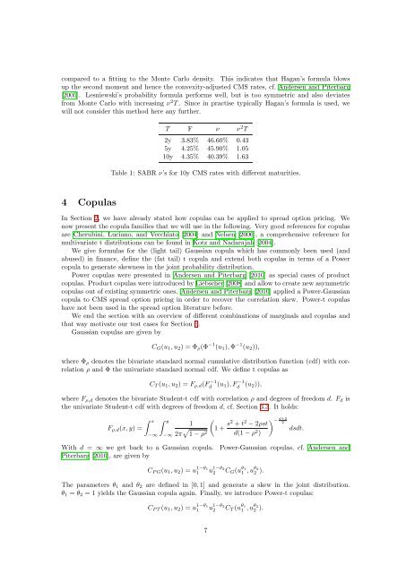
compared to a fitting to the Monte Carlo density. This indicates that Hagan’s formula blows up the second moment and hence the convexity-adjusted CMS rates, cf. Andersen and Piterbarg [2005]. Lesniewski’s probability formula performs well, but is too symmetric and also deviates from Monte Carlo with increasing ν 2 T . Since in practise typically Hagan’s formula is used, we will not consider this method here any further. 4 Copulas T F ν ν 2 T 2y 3.83% 46.60% 0.43 5y 4.25% 45.90% 1.05 10y 4.35% 40.39% 1.63 Table 1: SABR ν’s for 10y CMS rates with different maturities. In Section 2, we have already stated how copulas can be applied to spread option pricing. We now present the copula families that we will use in the following. Very good references for copulas are Cherubini, Luciano, and Vecchiato [2004] and Nelsen [2006], a comprehensive reference for multivariate t distributions can be found in Kotz and Nadarajah [2004]. We give formulas for the (light tail) Gaussian copula which has commonly been used (and abused) in finance, define the (fat tail) t copula and extend both copulas in terms of a Power copula to generate skewness in the joint probability distribution. Power copulas were presented in Andersen and Piterbarg [2010] as special cases of product copulas. Product copulas were introduced by Liebscher [2008] and allow to create new asymmetric copulas out of existing symmetric ones. Andersen and Piterbarg [2010] applied a Power-Gaussian copula to CMS spread option pricing in order to recover the correlation skew. Power-t copulas have not been used in the spread option literature before. We end the section with an overview of different combinations of marginals and copulas and that way motivate our test cases for Section 6. Gaussian copulas are given by CG(u1, u2) = Φρ(Φ −1 (u1), Φ −1 (u2)), where Φρ denotes the bivariate standard normal cumulative distribution function (cdf) with correlation ρ and Φ the univariate standard normal cdf. We define t copulas as CT (u1, u2) = Fρ,d(F −1 d (u1), F −1 d (u2)), where Fρ,d denotes the bivariate Student-t cdf with correlation ρ and degrees of freedom d. Fd is the univariate Student-t cdf with degrees of freedom d, cf. Section 3.3. It holds: Fρ,d(x, y) = x −∞ y −∞ 1 2π 1 − ρ 2 1 + s2 + t2 − 2ρst d(1 − ρ2 − ) d+2 2 dsdt. With d = ∞ we get back to a Gaussian copula. Power-Gaussian copulas, cf. Andersen and Piterbarg [2010], are given by CP G(u1, u2) = u 1−θ1 1 u 1−θ2 2 CG(u θ1 1 , uθ2 2 ). The parameters θ1 and θ2 are defined in [0, 1] and generate a skew in the joint distribution. θ1 = θ2 = 1 yields the Gaussian copula again. Finally, we introduce Power-t copulas: CP T (u1, u2) = u 1−θ1 1 7 u 1−θ2 2 CT (u θ1 1 , uθ2 2 ).
Page 1 and 2: Consistent Pricing of CMS and CMS S
Page 3 and 4: 2 The Pricing Problem Let S1 and S2
Page 5: Low Strikes: • β = 1: This case
Page 9 and 10: Figure 3: SABR densities of 10y CMS
Page 11 and 12: Figure 4: Joint densities for diffe
Page 13 and 14: • normal marginals and Gaussian c
Page 15 and 16: Figure 6: Comparison of 10y and 2y
Page 17 and 18: Figure 8: Power-Gaussian copula cal
Page 19 and 20: Figure 10: 10y2y spread digitals pr
Page 21 and 22: Figure 11: Fits of skewed-t distrib
Page 23 and 24: Figure 13: Joint densities generate
Page 25 and 26: = 2 ε + 1 0 ε = 2 ε + 1 ε wher
Page 27: A. Elices and J.P. Fouque. Perturbe

Consistent Pricing of CMS and CMS Spread Options - UniCredit ...

Create successful ePaper yourself

Delete template?

Save as template?