an mcnp primer - Kansas State University Mechanical and Nuclear ...

AN MCNP
PRIMER
by
J. K. Shultis
(jks@ksu.edu)
and
R. E. Faw
(fawre@triad.rr.com)
Dept. of Mechanical and Nuclear Engineering
Kansas State University
Manhattan, KS 66506
(c) Copyright 2004–2011
All Rights Reserved

Contents
1 Structure of the MCNP Input File 1
1.1 Annotating the Input File . . . . . . . . . . . . . . . . . . . . . . . . . . . . . . . . 1
1.2 Units Used by MCNP . . . . . . . . . . . . . . . . . . . . . . . . . . . . . . . . . . 2
2 Geometry Specifications 2
2.1 Surfaces – Block 2 . . . . . . . . . . . . . . . . . . . . . . . . . . . . . . . . . . . . 2
2.2 Cells – Block 1 . . . . . . . . . . . . . . . . . . . . . . . . . . . . . . . . . . . . . . 4
2.3 Macrobodies . . . . . . . . . . . . . . . . . . . . . . . . . . . . . . . . . . . . . . . 5
3 Data Specifications – Block 3 7
3.1 Materials Specification . . . . . . . . . . . . . . . . . . . . . . . . . . . . . . . . . . 7
3.2 Cross-Section Specification . . . . . . . . . . . . . . . . . . . . . . . . . . . . . . . 9
3.3 Source Specifications . . . . . . . . . . . . . . . . . . . . . . . . . . . . . . . . . . . 9
3.3.1 Point Isotropic Sources . . . . . . . . . . . . . . . . . . . . . . . . . . . . . 11
3.3.2 Isotropic Volumetric Sources . . . . . . . . . . . . . . . . . . . . . . . . . . 12
3.3.3 Line and Area Sources (Degenerate Volumetric Sources) . . . . . . . . . . . 12
3.3.4 Monodirectional and Collimated Sources . . . . . . . . . . . . . . . . . . . . 13
3.3.5 Multiple Volumetric Sources . . . . . . . . . . . . . . . . . . . . . . . . . . . 14
3.4 Tally Specifications . . . . . . . . . . . . . . . . . . . . . . . . . . . . . . . . . . . . 16
3.4.1 The Surface Current Tally (type F1) . . . . . . . . . . . . . . . . . . . . . . 16
3.4.2 The Average Surface Flux Tally (type F2) . . . . . . . . . . . . . . . . . . . 17
3.4.3 The Average Cell Flux Tally (type F4) . . . . . . . . . . . . . . . . . . . . . 17
3.4.4 Flux Tally at a Point or Ring (type F5) . . . . . . . . . . . . . . . . . . . . 17
3.4.5 Tally Specification Cards . . . . . . . . . . . . . . . . . . . . . . . . . . . . 17
3.4.6 Cards for Surface and Cell Tallies . . . . . . . . . . . . . . . . . . . . . . . . 18
3.4.7 Cards for Point-Detector Tallies . . . . . . . . . . . . . . . . . . . . . . . . 18
3.4.8 Cards for Optional Tally Features . . . . . . . . . . . . . . . . . . . . . . . 19
3.4.9 Miscellaneous Data Specifications . . . . . . . . . . . . . . . . . . . . . . . . 20
3.4.10 Short Cuts for Data Entry . . . . . . . . . . . . . . . . . . . . . . . . . . . . 20
3.5 Running MCNP . . . . . . . . . . . . . . . . . . . . . . . . . . . . . . . . . . . . . 20
3.5.1 Execution Options . . . . . . . . . . . . . . . . . . . . . . . . . . . . . . . . 20
3.5.2 Interrupting a Run . . . . . . . . . . . . . . . . . . . . . . . . . . . . . . . . 20
4 Variance Reduction 21
Revised December 12, 2011 An MCNP Primer i

4.1 Tally Variance . . . . . . . . . . . . . . . . . . . . . . . . . . . . . . . . . . . . . . 21
4.1.1 Relative Error and FOM . . . . . . . . . . . . . . . . . . . . . . . . . . . . . 22
4.2 Truncation Techniques . . . . . . . . . . . . . . . . . . . . . . . . . . . . . . . . . . 22
4.2.1 Energy, Time and Weight Cutoff . . . . . . . . . . . . . . . . . . . . . . . . 23
4.2.2 Physics Simplification . . . . . . . . . . . . . . . . . . . . . . . . . . . . . . 23
4.2.3 Histories and Time Cutoffs . . . . . . . . . . . . . . . . . . . . . . . . . . . 25
4.3 Nonanalog Simulation . . . . . . . . . . . . . . . . . . . . . . . . . . . . . . . . . . 25
4.3.1 Simple Examples . . . . . . . . . . . . . . . . . . . . . . . . . . . . . . . . . 25
4.4 MCNP Variance Reduction Techniques . . . . . . . . . . . . . . . . . . . . . . . . . 26
4.4.1 Geometry Splitting . . . . . . . . . . . . . . . . . . . . . . . . . . . . . . . . 27
4.4.2 Weight Windows . . . . . . . . . . . . . . . . . . . . . . . . . . . . . . . . . 28
4.4.3 An Example . . . . . . . . . . . . . . . . . . . . . . . . . . . . . . . . . . . 29
4.4.4 Exponential Transform . . . . . . . . . . . . . . . . . . . . . . . . . . . . . . 31
4.4.5 Energy Splitting/Russian Roulette . . . . . . . . . . . . . . . . . . . . . . . 32
4.4.6 Forced Collisions . . . . . . . . . . . . . . . . . . . . . . . . . . . . . . . . . 32
4.4.7 Source Biasing . . . . . . . . . . . . . . . . . . . . . . . . . . . . . . . . . . 32
4.5 Final Recommendations . . . . . . . . . . . . . . . . . . . . . . . . . . . . . . . . . 33
5 MCNP Output 33
5.1 Output Tables . . . . . . . . . . . . . . . . . . . . . . . . . . . . . . . . . . . . . . 33
5.2 Accuracy versus Precision . . . . . . . . . . . . . . . . . . . . . . . . . . . . . . . . 34
5.3 Statistics Produced by MCNP . . . . . . . . . . . . . . . . . . . . . . . . . . . . . . 35
5.3.1 Relative Error . . . . . . . . . . . . . . . . . . . . . . . . . . . . . . . . . . 35
5.3.2 Figure of Merit . . . . . . . . . . . . . . . . . . . . . . . . . . . . . . . . . . 35
5.3.3 Variance of the Variance . . . . . . . . . . . . . . . . . . . . . . . . . . . . . 36
5.3.4 The Empirical PDF for the Tally . . . . . . . . . . . . . . . . . . . . . . . . 36
5.3.5 Confidence Intervals . . . . . . . . . . . . . . . . . . . . . . . . . . . . . . . 38
5.3.6 A Conservative Tally Estimate . . . . . . . . . . . . . . . . . . . . . . . . . 38
5.3.7 The Ten Statistical Tests . . . . . . . . . . . . . . . . . . . . . . . . . . . . 39
5.3.8 Another Example Problem . . . . . . . . . . . . . . . . . . . . . . . . . . . 39
Revised December 12, 2011 An MCNP Primer ii

A Primer Presenting
AN INTRODUCTION TO THE MCNP CODE
J. Kenneth Shultis and Richard E. Faw
The MCNP Code, developed and maintained by Los Alamos National Laboratory, is the internationally
recognized code for analyzing the transport of neutrons and gamma rays (hence NP for
neutral particles) by the Monte Carlo method (hence MC). The code deals with transport of neutrons,
gamma rays, and coupled transport, i.e., transport of secondary gamma rays resulting from
neutron interactions. The MCNP code can also treat the transport of electrons, both primary source
electrons and secondary electrons created in gamma-ray interactions.
This tutorial document highlights certain aspects of the MCNP input code. The documentation
for the code is contained in 3 volumes. Volume I gives an overview (Ch. 1) and theory (Ch. 2) of the
code. Volume II is the User’s Guide that defines all the commands and options of the code (Ch. 3),
gives many examples (Ch. 4), and describes the code’s output (Ch. 5). Volume III is a Developer’s
Guide that gives many of the technical details of code and are needed by only the MCNP experts.
Some of the notation used in the MCNP documentation uses historical terminology. For example,
the term card, historically a punched card, should be interpreted as a line of the input file.
For the novice user, Ch. 1 of Vol. I of the manual presents an overview of MCNP that summarizes
the preparation of input files, the execution of the code, and the interpretation of results. This is
highly recommended reading. After gaining some experience with MCNP, the beginning user should
periodically browse through the remainder of Vol. I to obtain a better understanding of the theory
behind the many features of MCNP.
Volume II is essential for both the novice and expert user. This is the documentation that formally
defines all the commands and options that make MCNP such a powerful radiation transport code.
In this primer there are several margin notes indicating the pages in the MCNP5 manual that discuss Page nos. are
in more detail the subject being presented in this primer.
for MCNP5
The MCNP documentation is very comprehensive; thus, it is difficult for new users of the code
to distinguish between information essential to learning how to use the code and information needed
only under very specialized circumstances. For this reason, this tutorial document was prepared to
introduce the novice with the more basic (and essential) aspects of the MCNP code.
1 Structure of the MCNP Input File
An input file has the structure shown to the right.
Input lines have a maximum of 80 columns and
command mnemonics begin in the first 5 columns.
Free field format (one or more spaces separating
items on a line) is used and alphabetic characters
can be upper, lower, or mixed case. A continuation
line starts with 5 blank columns or a blank
followed by an & at the end of the card to be continued.
See pages 3-4 to 3-7 for more details on
formatting input cards.
1.1 Annotating the Input File
Message Block +
blank line delimiter {optional}
One Line Problem Title Card
Cell Cards [Block 1]
blank line delimiter
Surface Cards [Block 2]
blank line delimiter
Data Cards [Block 3]
blank line terminator {optional}
It is good practice to add comments liberally to an input MCNP file so that it is easier for you and
others to understand what problem is addressed and the tricks used. A comment line begins with
C or c followed by a space. Such a line is ignored by MCNP. Alternatively, anything following a $
sign on a line is ignored. See Fig. 5 on page 30 for a well-annotated MCNP input file.
Revised December 12, 2011 An MCNP Primer 1

1.2 Units Used by MCNP
The units used by MCNP are (1) length in cm, (2) energy in MeV, (3) time in shakes (10 −8 s), (4)
temperature in MeV (kT), (5) atom density in atoms b −1 cm −1 , (6) mass density in g cm −3 , and
(7) cross sections in barns.
2 Geometry Specifications
The specification of problem geometry is treated in several sections of the MCNP manual. In Vol. I,
beginning on page 1-12, there is an introduction to geometric specification. Discussion continues in
Ch. 2 Sec. II (page 2-7). Sections II and III of Ch. 3 provide detailed instructions on preparation of
problem input cards and Finally, Ch. 4 Sec. I provides many examples of geometry specifications.
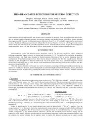
MCNP treats problem geometry primarily in terms of regions or volumes bounded by first and
second degree surfaces. Cells are defined by intersections, unions, and complements of the regions,
and contained user defined materials. The intersection and union of two regions A and B are shown
by the shaded regions in Fig. 1.
The union operation may be thought of as a logical OR, in that the union of A and B is a
new region containing all space either in region A OR region B. The intersection operation may
be thought of as a logical AND, in that the result is a region that contains only space common to
both A AND B. The complement operator # plays the roll of a logical NOT. For example # (A:B)
represents all space outside the union of A and B.
A:B AB
Figure 1. Left: the union A:B or “A or B”. Right: the intersection A B or “A and B”.
MCNP uses a 3-dimensional (x, y, z) Cartesian coordinate system. All dimensions are in centimeters
(cm). All space is composed of contiguous volumes or cells. Each cell is bounded by a surface,
multiple surfaces, or by infinity. For example, a cube is bounded by six planes. Every (x, y, z) point
must belong to a cell (or be on the surface of a cell). There can be no “gaps” in the geometry, i.e.,
there can be no points that belong to no cell or surface. Every cell and surface is given by the user
a unique numerical identifier.
2.1 Surfaces – Block 2
Table 1, taken from the MCNP manual, lists the surfaces used by MCNP to create the geometry
of a problem. All refer to a Cartesian coordinate system. A surface is represented functionally
as f(x, y, z) = 0. For example, for a cylinder of radius R parallel to the z-axis is defined as
f(x, y, z) =(x− ¯x) 2 +(y − ¯y) 2 − R2 , where the cylinder’s axis is parallel to the z-axis and passes
through the point (¯x, ¯y, 0). The MCNP input line for such a surface, which is denoted by the
mnemonic C/Z (or c/z, since MCNP is case insensitive), is
1 C/Z 5 5 10 $ a cylindrical surface parallel to z-axis
defines surface 1 as an infinitely long cylindrical surface parallel to z-axis with radius 10 cm and
whose axis passes through the point (x =5cm,y =5cm,z = 0). Note that the length of the
cylinder is infinite. Note also the in-line comment, introduced by the $ symbol.
Revised December 12, 2011 An MCNP Primer 2

Table 1. MCNP Surface Cards (page 3-13 of MCNP5 manual)
Mnemonic Type Description Equation Card Entries
P plane general Ax + By + Cz − D =0 ABCD
PX normal to x-axis x − D =0 D
PY normal to y-axis y − D =0 D
PZ normal to z-axis z − D =0 D
SO sphere centered at origin x 2 + y 2 + z 2 − R 2 =0 R
S general (x−¯x) 2 +(y−¯y) 2 +(z−¯z) 2 −R 2 =0 ¯x ¯y ¯z R
SX centered on x-axis (x − ¯x) 2 + y 2 + z 2 − R 2 =0 ¯x R
SY centered on y-axis x 2 +(y − ¯y) 2 + z 2 − R 2 =0 ¯y R
SZ centered on z-axis x 2 + y 2 +(z − ¯z) 2 − R 2 =0 ¯z R
C/X cylinder parallel to x-axis (y − ¯y) 2 +(z − ¯z) 2 − R 2 =0 ¯y ¯z R
C/Y parallel to y-axis (x − ¯x) 2 +(z − ¯z) 2 − R 2 =0 ¯x ¯z R
C/Z parallel to z-axis (x − ¯x) 2 +(y − ¯y) 2 − R 2 =0 ¯x ¯y R
CX on x-axis y 2 + z 2 − R 2 =0 R
CY on y-axis x 2 + z 2 − R 2 =0 R
CZ on z-axis x 2 + y 2 − R 2 =0 R
K/X cone parallel to x-axis (y−¯y) 2 +(z−¯z) 2 − t(x−¯x) =0 ¯x ¯y ¯z t2 ± 1
K/Y parallel to y-axis (x−¯x) 2 +(z−¯z) 2 − t(y−¯y) =0 ¯x¯y ¯z t2 ± 1
K/Z parallel to z-axis (x−¯x) 2 +(y−¯y) 2 − t(z−¯z) =0 ¯x¯y ¯z t2 ± 1
KX on x-axis
y2 + z2 2 − t(x − ¯x) =0 ¯x t ± 1
KY on y-axis
KZ on z-axis
√ x 2 + z 2 − t(y − ¯y) =0 ¯y t 2 ± 1
x 2 + y 2 − t(z − ¯z) =0 ¯z t 2 ± 1
±1 used only for 1-sheet cone
SQ ellipsoid axis parallel A(x − ¯x) 2 + B(y − ¯y) 2 + C(z − ¯z) 2 ABCDE
hyperboloid to x-, y-, or z-axis +2D(x − ¯x)+2E(y − ¯y) FG¯x ¯y ¯z
paraboloid +2F (z − ¯z)+G =0
GQ cylinder, cone axis not parallel Ax 2 + By 2 + Cz 2 + Dxy + Eyz ABCDE
ellipsoid to x-, y-, or z-axis +Fzx+ Gz + Hy + Jz + K =0 FGHJK
paraboloid
hyperboloid
TX elliptical or (x−¯x) 2 /B 2 +( (y−¯y) 2 +(z−¯z) 2 − A) 2 /C 2 − 1=0 ¯x ¯y ¯zA BC
circular torus.
TY Axis is (y−¯y) 2 /B 2 +( (x−¯x) 2 +(z−¯z) 2 − A) 2 /C 2 − 1=0 ¯x ¯y ¯zA BC
parallel to x-,
TZ y-, or z-axis (z−¯z) 2 /B 2 +( (x−¯x) 2 +(y−¯y) 2 − A) 2 /C 2 − 1=0 ¯x ¯y ¯zA BC
XYZP surfaces defined by points – see pages 3-15 to 3-17
Revised December 12, 2011 An MCNP Primer 3

Every surface has a “positive” side and a “negative” side. These directional senses for a surface
are defined formally as follows: any point at which f(x, y, z) > 0 is located in the positive sense
(+) to the surface, and any point at which f(x, y, z) < 0 is located in the negative sense (−) to the
surface. For example, a region within a cylindrical surface is negative with respect to the surface
and a region outside the cylindrical surface is positive with respect to the surface.
2.2 Cells – Block 1
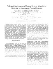
We illustrate how surfaces and Boolean logic are used to define cells by considering a simple example
of a cylindrical storage cask whose wall and ends are composed of iron 1-cm thick. Inside and outside
the cask are void regions. Suppose the outer cylindrical surface is that used in the illustration in
the previous section. The geometry for this problem is shown in Fig. 2.
z=60
z=59
9
z=41
z=40
7
x
z
Figure 2. Geometry for a simple cylindrical cask. Numbers in
triangles are surface identification numbers and numbers in circles
define the cell identification number. The axis of the cask passes
through the point (x = 5 cm, y = 5 cm) and the cask outer radius
is 10 cm.
To define the inside surface of the cask, we need another cylinder inside and concentric with the
first cylinder but with a radius smaller by 1 cm. We shall call this smaller cylindrical surface number
4, so that the surface definition lines in the input file for these two cylinders are
1 C/Z 5 5 10 $ outer cylindrical surface
4 C/Z 5 5 9 $ inner cylindrical surface
To define the base and top of the cask, planes perpendicular to the z-axis are needed at locations
z = 40 cm and z = 60 cm, respectively. Similarly, to define the base and top of the inner cavity
of the cask two more planes perpendicular to the z-axis are needed at z = 41 cm and z = 59 cm.
These four planes are defined by
2 PZ 40 $ base of cask
3 PZ 60 $ top of cask
5 PZ 41 $ base of inner cavity
6 PZ 59 $ top of inner cavity
These six surface definition cards (or input lines) can appear in any order in Block 2 of the input
file.
Revised December 12, 2011 An MCNP Primer 4
9
2
8
6
y
5
3
9
4
1
9

With the problem surfaces defined, we now begin to define the volumes or cells which must fill
all (x, y, z) space. These cell definition cards comprise the content of Block 1 of the input file. First,
we define the inner void of the cask as cell 8. This volume is negative with respect to surface 4,
positive with respect to the plane 5, and negative with respect to plane 6. Thus, cell 8 is defined as
8 0 -4 5 -6 IMP:N=0 IMP:P=1 $ inner cask void
The first number on a cell definition card is the cell number (arbitrarily picked by the user). Here
the second entry 0 denotes that the cell is filled by a void, and -4 5 -6 indicate that all points in
cell 8 are inside the cylinder 4 AND are above plane 5 AND are below plane 6. region. The last
two IMP specifications define the importance of this region to neutrons (N) and (P). Neutrons in this
cell have zero weight and photons have unit weight (e.g., for a photon transport problem). We’ll
discuss importances later. The order of surfaces in an intersection string is immaterial. Thus, we
could have defined cell 8 by intersection of surfaces -6 -4 5.
Now consider the iron shell of the cask. Suppose this cell is given 7 as its id number and consists
of material 5, as yet to be defined, with density 7.86 g/cm3 . Space within this cell is negative with
respect to surface 1, positive with respect to surface 2 and negative with respect to surface 3 AND
also cannot be inside the void or cell 8. This cell can thus be define as
7 5 -7.86 -1 2 -3 #8 IMP:N=0 IMP:P=1 $ iron cask shell
Although the complement operator # (for NOT) is often a convenient way to exclude an inner region,
this operator often reduces the efficiency of MCNP. In fact, theoretically one never has to use #.
The region outside cell 8 can be defined by the union string (4:6:-5) and the definition of cell 7
can be equivalently defined as
7 5 -7.86 -1 2 -3 (4:6:-5) IMP:N=0 IMP:P=1 $ iron cask shell
Now suppose that cells 7 and 8 describe all space of interest for radiation transport. In other
words, suppose that all photons passing outside the outer surface of the finite cylinder may be killed,
i.e., their path tracking can be ended. One still needs to assign this space to a cell. Further by setting
the photon importance in this cell to zero, any photon entering is killed. This “graveyard” cell, say
cell 9, is the union of all regions positive with respect to surfaces 1 and 3 and negative with respect
to surface 2. Hence the graveyard is defined by
9 0 1:3:-2 IMP:N=0 IMP:P=0 $ graveyard
The graveyard could also be defined by using the complement operator and by specifying that
the kill zone is all space outside the union of cells 7 and 8, namely
9 0 #(7:8) IMP:N=0 IMP:P=0 $ graveyard
Note that the second entry on this cell card is zero, indicating a vacuum and that the photon
importance is set to zero.
2.3 Macrobodies
MCNP has an alternative way to define cells and surfaces through the use of macrobodies. These
macrobodies can be mixed with the standard cells and surfaces and are defined in Block 2. For
example, the command in Block 2
3-18 to 3-23
15 RCC 1 2 5 0 0 50 10 $ right circular cylinder
defines a right circular cylinder with the following properties: the center of the base is at (1,2,5);
the height is 50 cm and the axis is parallel to the z-axis; the radius is 10 cm; and the macrobody
has 15 as its identifier.
The macrobodies available in MCNP are shown in Table 2. MCNP automatically decomposes the
macrobody surface into surface equations and the facets are assigned identifying numbers according
to a predetermined sequence. The assigned surface number consists of the macrobody identifier
number follow by a decimal point and an integer 1, 2,... . For example in the RCC example above,
the cylindrical surface has the identifier 15.1, the plane of the top is 15.2, and the plane of the base
Revised December 12, 2011 An MCNP Primer 5

Table 2. Macrobodies available in MCNP.
Mnemonic Type of body
BOX arbitrarily oriented orthogonal box (90 ◦ corners)
RPP rectangular paralleliped (surfaces parallel to axes)
SPH sphere
RCC right circular cylinder
RHP or HEX right hexagonal prism
REC right elliptical cylinder
TRC truncated right-angle cone
ELL ellipsoid
WED wedge
ARB arbitrary polyhedron
is 15.3. These facet surfaces can be used for anything standard surfaces are used for, e.g., tallies,
other cell definitions, source definitions, etc.
The definition of a macrobody requires many parameters. Here we give the details for three of
the most useful macrobodies.
BOX Arbitrarily oriented orthogonal box: This body is defined by four vectors: v defining a
corner of the box and three orthogonal vectors a, b, and c defining the length and direction of the
sides from the specified corner. The syntax is
BOX vx vy vz ax ay az bx by bz cx cy cz
The facet suffixes are: .1/.2 plane perpendicular to the end/beginning of a
.3/.4 plane perpendicular to the end/beginning of b
.5/.6 plane perpendicular to the end/beginning of c
RPP Rectangular parallelepiped: This orthogonal box has sides perpendicular to the coordinate
axes. This body is defined by the range each side has along its parallel axis. The syntax is
RPP xmin xmax ymin ymax zmin zmax
The facet suffixes are: .1/.2 plane xmax/xmin; .3/.4 plane ymax/ymin; .5/.6 plane zmax/zmin.
RCC right circular cylinder: This right cylinder is defined by a vector v that gives the center of
the base, a vector h that defines the axis and height of the cylinder, and the radius R. The syntax
is RCC vx vy vz hx hy hz R
The facet suffixes are: .1 cylindrical surface; .2/.3 plane normal to the end/beginning of h.
The space inside a macrobody has a negative sense with repsect to the macrobody surface and
all its facets. The space outside has a positive sense. More important to remeber is that the sense
of a facet is the sense assigned to it by the macrobody and the facet surface retains this sense if
it appears in other cell definitions. For example, the base of the RCC cylinder discussed above is
a plane normal to the z-axis with intercept of 5 cm and has the identifier 15.3. The space with
z>5 has a negative sense to this surface because this space is towards the interior of the cylinder.
The space for z5 has a positive
sense with respect to surface 16 while it has a negative sense for surface 15.3!
The use of macrobodies can greatly ease the specification of a problem’s geometry. We illustrate
this by returning to the simple cask problem considered in the previous section. Rather than define
Revised December 12, 2011 An MCNP Primer 6

z=60
z=59
9
z=41
z=40
7
x
z
9
8
y
9
MB 17
MB 18
Figure 3. Geometry for a simple cylindrical cask. Two macrobody right cylinders
are used to define the inside and ouside surfaces of the cask and numbers in circles
are the cell identification number. As before, the axis of the cask passes through
the point (x = 5 cm, y = 5 cm, z =0)
6 surfaces to form the cask, we use two nested cylinder macrobodies. The subsequent Boolean logic
used to define the three cells now becomes considerably simpler. For the geometry shown in Fig. 3,
the input geometry specification becomes
Use of macrobodies for cask problem
c ***************** BLOCK 1 -- cells
8 0 -18 IMP:P,N=1 $ inside the cask
7 5 -7.86 18 -17 IMP:P,N=1 $ cask iron shell
9 0 17 IMP:P,N=0 $ void outside cask
c ***************** BLOCK 2 -- surfaces/macrobodies
17 RCC 5 5 40 0 0 20 10 $ outer cylinder
18 RCC 5 5 41 0 0 18 9 $ inner cylinder
Cell 8 is simply all the space inside macrobody 18 and is denoted by -18. Cell 7 is all the space inside
macrobody 17 and outside macrobody 18, namely 18 -17. These cell definitions are considerably
simpler than those based on the intersections and unions of the six standard surfaces used in the
previous definition of this cask.
3 Data Specifications – Block 3
This block of input cards defines the type of particles, problem materials, radiation sources, how
results are to be scored (or tallied), the level of detail for the physics of particle interactions, variance
reduction techniques, cross section libraries, the amount and type of output, and much more. In
short, this third input block provides almost all problem specifications other than the geometry
An introduction to Block 3 commands is provided in Vol. II pp. 1-5 to 1-10. Detail on the
theory behind the many program options is provided in Ch. 2 Secs. III through V. Section IV of
Ch. 3 provide detailed instructions on preparation of problem input cards and Ch. 4 Secs. IV and
V provides examples of source and tally treatments.
3.1 Materials Specification
Specification of materials filling the various cells in an MCNP calculation involves the following 3-114 to
elements: (a) defining a unique material number, (b) the elemental (or isotopic) composition, and
(c) the cross section compilations to be used.
3-124
Revised December 12, 2011 An MCNP Primer 7
9

Note that density is not specified here. Instead, density is specified on the cell definition card.
This permits one material to appear at different densities in different cells. Suppose that the first
material to be identified in problem input is (light) water and that only gamma-ray transport is of
interest. Comment cards (cards beginning with C or c) may be used for narrative descriptions. In
the following card images, the designation M1 refers to material 1. For a compound, unnormalized
atomic fractions may be used. For example,
c -------------------------------------------------------c
WATER for gamma-ray transport (by atom fraction)
c ---------------------------------------------------------
M1 1000 2 $ elemental H and atomic abundance
8000 1 $ elemental O and atomic abundance
The designations 1000 and 8000 identify elemental hydrogen, atomic number Z = 1, and elemental
oxygen (Z = 8). The three zeros in each designation are place holders for the atomic mass
number, which would be required to identify specific isotopes of the element and which, generally,
are required for neutron transport, as described later. For gamma ray and electron transport, one
need only specify the atomic number. For compounds or mixtures, composition may alternatively
be specified by mass fraction, indicated by a minus sign, as follows
c -------------------------------------------------------c
WATER for gamma-ray transport (by mass fraction)
c ---------------------------------------------------------
M1 1000 -0.11190 $ elemental H mass fraction
8000 -0.88810 $ elemental O mass fraction
Error/warning messages can be avoided by assuring that mass/atomic fractions sum to unity.
For neutron transport problems, often a specific isotope of an element must be specified. The
isotope ZAID number (Z AIDentification) contains six digits ZZZAAA in which ZZZ is the atomic
number Z and AAA is the atomic mass number A. Thus 235U has a ZAID number 092235 or simply
92235. If neutron cross sections for an element composed of its isotopes in their naturally occurring
abundances is desired, then the ZAID is specified as ZZZ000. Note, such elemental neutron cross
section sets are not available for all elements. Often you must list all the important isotopes. As an
example, light water for neutron problems could be defined as
c -------------------------------------------------------c
WATER for neutron transport (by mass fraction)
c (ignore H-2, H-3, O-17, and O-18)
c ---------------------------------------------------------
M1 1001.60c -0.11190 $ H-1 and mass fraction
8016.60c -0.88810 $ O-16 and mass fraction
Here 1001 and 8016 provide atomic number and atomic mass designations, in the form of the
ZAID numbers. The .60c designation identifies a particular cross section compilation (see Section 3.2
below).
When hydrogen is molecularly bound in water, either pure or as a constituent in some other
material, the binding affects energy loss in collisions experienced by slow neutrons. For this reason,
special cross-section data treatments are provided that take binding effects into account. To use this
special treatment, an additional MT card is required, as shown below.
c -------------------------------------------------------c
WATER for neutron transport (by mass fraction)
c (ignore H-2, H-3, O-17, and O-18)
c Specify S(alpha,beta) treatment for binding effects
c ---------------------------------------------------------
M1 1001.50c -0.11190 $ H-1 and mass fraction
8016.50c -0.88810 $ O-16 and mass fraction
MT1 lwtr.01
Revised December 12, 2011 An MCNP Primer 8

Without the MT card, hydrogen would be treated as if it were a monatomic gas. Treatment of binding
effects for other nuclides and other materials is described in Appendix G of Vol. I of the MCNP
manual.
3.2 Cross-Section Specification
Neutron reactions and cross-section data tables are described in Section III of Chapter 2 in the MCNP
manual. A comprehensive list of cross section compilations is provided in Table G2 of Appendix
G (part of Vol. I). Specification of a particular cross-section compilation depends somewhat on the
nature of the problem being solved and on the data available to the user. Not all cross section
sets are available to all users. For users obtaining data through the Radiation Safety Information
Computation Center (RSICC), a common choice would be the .66c cross sections available in the
endf66 library which is derived from the ENDF/B-VI evaluated nuclear data files.
In some instances, cross sections are available for elements with naturally occurring atomic
abundances. For example, natural chromium would be identified by ZAID 24000.60c. However,
cross sections for the isotope 50 Cr would require the identification 24050.60c and would require the
endf60 library containing data from the ENDF/B-VI evaluated nuclear data file. The ENDF/B-VI
cross sections are included with the MCNP-5 distribution package. In some instances, it is necessary
for the user to define a natural element as a combination of isotopes. This is the case for many of
the light elements such as helium and lithium.
3.3 Source Specifications
The source and type of radiation particles for an MCNP problem are specified by the SDEF com- 3-51 to 3-77
mand. The SDEF command has many variables or parameters that are used to define all the
characteristics of all sources in the problem. The SDEF command with its many variables is one of
the more complex MCNP commands and is capable of producing an incredible variety of sources —
all with a single SDEF command. And only one SDEF card is allowed in an input file.
On the SDEF line values of the variables in Table 3 are entered, if other than the default values,
that are needed to characterize the source. The = sign is optional, so that PAR=1 is equivalent to
PAR 1. Values of variables can be specified at three levels: (1) explicitly (e.g., ERG=1.25), (2) with
a distribution number (e.g., ERG=d5), and (3) as a function of another variable (e.g., ERG=Fpos).
Specifying variables at levels 2 and 3 requires the use of three other source cards: the SI (source
information) card, the SP (source probabilities) card, and the SB (source bias) card.
Section D of Ch. 3 gives a complete description of the SDEF command and the use of its
variables. This is a very tersely written section and it is very difficult for the novice to understand
all the features and subtleties. As an MCNP user gains experience, this section should be periodically
reread. Each reading almost always provides new insight and understanding of the SDEF command.
Chapter 4 of the MCNP manual has several examples of complicated sources. These are well
worth studying. However, we often need fairly simple sources and such examples are not provided
in the MCNP manual. It takes many readings of the few pages in Chapter 3 describing all the
source commands and options to sometimes see how to do something fairly simple. Below are a few
examples of fairly simple source definitions that may help you to understand better how to specify
sources for MCNP.
When developing a new source definition, always check and recheck that source particles are
truly being generated where you think they should be. HINT: Always use the VOID card and the
PRINT 110 statement somewhere in block 3 of the input file. The PRINT 110 causes the starting
locations. directions, and energies of the first 50 particles to be printed to the output file. Examine
this output table to convince yourself that particles are being generated as you expect.
Revised December 12, 2011 An MCNP Primer 9

Table 3. Source variables for the SDEF command (page 3-53).
Variable Meaning Default
CEL cell determined from XXX, YYY, ZZZ and possibly UUU,
VVV, WWW
SUR surface 0 (means cell source)
ERG energy (MeV) 14 MeV
DIR µ, the cosine of the angle between
VEC and UUU, VVV, WWW. The
azimuthal angle is always sampled
uniformly in [0, 2π]
Volume case: µ is sampled uniformly in [−1.1]
(isotropic). Surface case: p(µ) =2µ for µɛ[0, 1] (cosine
distribution).
VEC reference vector for VEC Volume case: required unless isotropic. Surface case:
vector normal to the surface with sign determoined by
NRM.
NRM sign of the surface normal +1
POS reference
sampling
point for positioning 0, 0, 0
RAD radial distance of the position from
POS or AXS
0
EXT Cell case: distance from POS along
AXS. Surface case: cosine of angle
from AXS
0
AXS reference vector for EXT and RAD no direction
X x-coordinate of position no X
Y y-coordinate of position no Y
Z z-coordinate of position no Z
CCC cookie-cutter cell no cookie-cutter cell
ARA area of surface (required only for direct
contributions to point detectors
from a plane surface source
none
WGT particle weight 1
EFF reference efficiency criterion for position
sampling
0.01
PAR type of particle source emits = 1 (neutron) if MODE N or P or N P E; = 2 (photon)
if MODE P; = 3 (electron) if MODE E
Revised December 12, 2011 An MCNP Primer 10

3.3.1 Point Isotropic Sources
Two Point Isotropic Sources at Different Positions
c ----- Source: two point isotropic 1-MeV photon sources on x-axis
SDEF ERG=1.00 PAR=2 POS=d5 $ energy, particle type, location
SI5 L -10 0 0 10 0 0 $ (x,y,z) coords of the two pt sources
SP5 .75 .25 $ relative strengths of each source
Point Isotropic Source with Discrete Energy Photons
c ----- Source: point isotropic source with 4 discrete photon energies
SDEF POS 0 0 0 ERG=d1 PAR=2
SI1 L .3 .5 1. 2.5 $ the 4 discrete energies (MeV)
SP1 .2 .1 .3 .4 $ frequency of each energy
.4
.2
-10
z
freq
y
E 1 E 2 E 3 E 4
Point Isotropic Source with a Histogram of Energies
c ----- source: point isotropic with 4 histogram energy bins
SDEF POS 0 0 0 PAR=2 ERG=d1 $ position, particle type, energy
.4
N(E)
SI1 H
SP1 D
.1
0
.3
.2
.5
.4
1.
.3
2.5
.1
$ histogram boundaries
$ probabilities for each bin
.2
E
Point Isotropic Source with a Continuum of Energies
c ----- source: point isotropic with Maxwellian energy spectrum
SDEF POS 0 0 0 PAR=2 ERG=d1 $ position, particle type, energy
SP1 -2 0.5 $ Maxwellian spectrum (2) with temp a=0.5 MeV
Point Isotropic Source with Tabulated Energy Distribution
c ----- source: continuum energies tabulated at discrete energies
SDEF POS 0 0 0 PAR=2 ERG=d1 $ position, particle type, energy
SI1 A 1 2 3 4 5.5 7.0 7.5 $ tabulated energies E1 ... E7
SP1 0 .2 .27 .3 .28 .18 0 $ distrbution values f(Ei)
Two Point Sources with Different Energy Distributions
c --- 2 pt iso sources: src 1 (4-bins) src 2 (4 discrete Ei)
SDEF PAR=2 POS=d1 ERG FPOS d2
SI1 L
SP1
-10 0 0
.4
10 0 0
.6
$ coords of srcs on x-axis
$ rel strengths of sources
.4
DS2 S 3 4 $ energy distributions .2
SI3 H .1 .3 .5 1. 2.5 $ E bin limits src 1
SP3 D 0 .2 .4 .3 .1 $ bin prob for src 1
SI4 L .3 .5 .9 1.25 $ discrete Ei for src 2
SP4 .20 .10 .30 .40 $ rel freq for src 2
N(E)
.4
.2
N(E)
f(E )
i
E 1 E 2 E 3 E 4
.4
.2
freq
10
E 5 E 6E 7
-10 0 10
source 1 source 2
Revised December 12, 2011 An MCNP Primer 11
E
E
x
E
E
E
x

3.3.2 Isotropic Volumetric Sources
Rectangular Parallelepiped Parallel to Axes
c --- volumetric monoenergetic source inside a rectangular parallelepiped
SDEF X=d1 Y=d2 Z=d3 ERG=1.25 PAR=2
SI1 -10. 10. $ x-range limits for source volume
SP1 0 1 $ uniform probability over x-range
SI2 -15. 15.
SP2 0 1
$ y-range limits for source volume
$ uniform probability over y-range y
SI3 -20. 20. $ z-range limits for source volume
SP3 0 1 $ uniform probability over z-range x
Source in a Complex Cell: Enclosing Parallelepiped Rejection Method
c --- Cell 8 is some complex cell in which a monoenergetic isotropic
c volumetric source exists. A rectangular parallelepiped envelops
c this cell (MCNP does NOT check this!). Points, randomly picked
c in the rectangular parallelepiped, are accepted as source points
c
c
only if they are inside cell 8.
SDEF X=d1 Y=d2 Z=d3 ERG=1.25 PAR=2 CEL=8
c NOTE: source parallelepiped is larger that cell 8, and hence
c source positions sampled outside cell 8 are rejected.
SI1 -12. 12. $ x-range limits for source volume
SP1 0 1 $ uniform probability over x-range
SI2 -11. 11.
SP2 0 1
$ y-range limits for source volume
$ uniform probability over y-range
cell 8
SI3 -13. 13. $ z-range limits for source volume
SP3 0 1 $ uniform probability over z-range
Source in a Complex Cell: Enclosing Sphere Rejection Method
c --- Cell 8 is some complex cell in which a monoenergetic isotropic
c volumetric source exists. A sphere envelops this cell {MCNP
c does NOT check this!). Points, randomly picked in the sphere,
c
c
are accepted as source points only if they are inside cell 8.
SDEF POS=0 0 0 RAD=d1 CEL=8
SI1 0 20. $ radial sampling range: 0 to Rmax (=20cm)
SP1 -21 2 $ weighting for radial sampling: here r^2
3.3.3 Line and Area Sources (Degenerate Volumetric Sources)
Line Source (Degenerate Rectangular Parallelepiped)
c --- Line monoenergetic photon source lying along x-axis
c
c
This uses a degenerate Cartesian volumetric source.
SDEF POS=0 0 0 X=d1 Y=0 Z=0 PAR=2 ERG=1.25
SI1 -10 10 $ Xmin to Xmax for line source
-10
SP1 -21 0 $ uniform sampling on line Here x^0 z
Revised December 12, 2011 An MCNP Primer 12
z
cell 8
y
10
x

Disk Source (Degenerate Cylindrical Source)
c --- disk source in x-y plane centered at the origin.
c
c
This is a degenerate cylindrical volume source.
SDEF POS=0 0 0 AXS=0 0 1 EXT=0 RAD=d1 PAR=2 ERG=1.25
SI1 0 11 $ radial sampling range: 0 to Rmax
SP1 -21 1 $ radial sampling weighting: r^1 for disk source
Plane Source (Degenerate Rectangular Parallelepiped)
c --- rectangular plane source centered on the origin and perpendicular
c
c
to the y-axis. This uses a degenerate Cartesian volumetric source.
SDEF POS=0 0 0 X=d1 Y=d2 Z=0 PAR=2 ERG=1.25
SI1 -10 10 $ sampling range Xmin to Xmax
SP1 0 1 $ weighting for x sampling: here constant
SI2 -15 15 $ sampling range Ymin to Ymax
SP2 0 1 $ weighting for y sampling: here constant
Line Source (Degenerate Cylindrical Source)
c --- line source (degenerate cylindrical volumetric source)
SDEF pos=0 0 0 axs=1 0 0 ext=d1 rad=0 par=2 erg=1.25
SI1 -10 10 $ axial sampling range: -X to X
SP1 -21 0 $ weighting for axial sampling: here constant
3.3.4 Monodirectional and Collimated Sources
Monodirectional Disk Source
c --- Disk source perpendicular to z-axis uniformly emitting
c 1.2-MeV neutrons monodirectionally in the +ve z-direction.
c
SDEF POS=0 0 0 AXS=0 0 1 EXT=0 RAD=d1 PAR=1 ERG=1.2
VEC=0 0 1 DIR=1
SI1 0 15 $ radial sampling range: 0 to Rmax (=15cm)
SP1 -21 1 $ radial sampling weighting: r^1 for disk
Point Source Collimated into a Cone of Directions
c --- Point isotropic 1.5-MeV photon source collimated into
c an upward cone. Particles are confined to an upward
c (+z axis) cone whose half-angle is acos(0.9) = 25.8
c degrees about the z-axis. Angles are with respect to
c
c
the vector specified by VEC
SDEF POS=0 0 0 ERG=1.25 PAR=2 VEC=0 0 1 DIR=d1
SI1 -1 0.9 1 $ histogram for cosine bin limits
SP1 0 0.95 0.05 $ frac. solid angle for each bin
SB1 0. 0. 1. $ source bias for each bin
With this conical source, tally normalization is per source particle in 4π steradians. To normalize
the tally per source particle in the cone, put WGT=1/fsa2 on the SDEF card, where fsa2 is the
fraction solid angle of the cone (0.05 in the above example).
Revised December 12, 2011 An MCNP Primer 13
x
x
-10
x
x
z
z
z
z
z
y
R max
10
y
y
y
y
x

This conical collimation trick can also be used to preferentially bias the emission of particles in
certain directions. The SIn entries are the upper bin cosine limits µi ≡ cos θi in ascending order.
The first entry is −1. Angles are with respect to the direction specified by VEC. The SPn entries
give the fractional solid angle fsai = [(1 − µi−1) − (1 − µi)]/2 for the bin from µi−1 to µi, and the
SBn entries give the desired relative probabilities for emission in each angular bin. Note the first
probability must be 0 for the unrealistic bin from (−∞, −1).
3.3.5 Multiple Volumetric Sources
Two Cylindrical Volumetric Sources
c --- 2 volumetric sources uniformly distributed in cells 8 & 9.
c Both sources emit-1.25 MeV photons. Surround both source cells
c by a large sampling cylinder defined by the POS RAD and EXT
c parameters. The rejection technique is used to pick source
c
c
points with cells 8 and 9 with the specified frequency.
SDEF ERG=1.25 CEL d1 AXS=0 0 1 POS 0 0 0 RAD d2 EXT d5
SI1 L 8 9 $ source cells: src 1 =cell 8, src 2 =cell 9
SP1 0.8 0.2 $ 80% from src 1; 20% from src 2
SI2 0 50 $ radius of cyl. containing cells 8 & 9
SI5 -30 30 $ axial range of cyl. containing src cells
Two Cylindrical Sources with Different Energy Photons
c --- Two spatially different cylindrical monoenergetic sources.
c The size and position of each cyl. source depends on the
c
c
source energy (FERG).
SDEF ERG=d1
c
POS=FERG d8 AXS=0 0 1 RAD=FERG d2 EXT=FERG d5
c -- set source energies: .667 MeV for region 1 and 1.25 MeV for region 2
SI1 L 0.667 1.25 $ fix energies: .667 MeV for region 1 and 1.25 MeV for region 2
SP1 0.4 0.6 $ 20% from src 1(Cs-137); 80% from src 2 (Co-60)
c -- set positions of the 2 source cylinders
DS8 S 9 10 $ get postion for chosen source
z
SI9 L -30 0 0 $ center for sampling of src 1
SP9 1 $ prob. distn for src 1 center
SI10 L 30 0 0 $ center for sampling of src 2
SP10 1 $ prob. distn for src 2 center
c -- set radius and axial limits for each source
DS2 S 3 4 $ sampling distns from each src axis
SI3 0 20 $ radial sampling limits for src1
-30
sourse 1
x
SP3 -21 1 $ radial sampling weight for src1 r^1
SI4 0 10 $ radial sampling limits for src2
SP4 -21 1 $ radial sampling weight for src2 r^1
DS5 S 6 7 $ axial sampling distns for each src
SI6 -10 10 $ axial sampling limits for src1
SP6 -21 0 $ axial sampling weight for src1 r^0
SI7 -30 30 $ axial sampling limits for src2
SP7 -21 0 $ axial sampling weight for src2 r^0
Revised December 12, 2011 An MCNP Primer 14
x
8
z
9
sampling
cylinder
30
y
y
source 2

Two Arbitrary Volumetric Sources with Different Energy Photons
c --- 2 volumetric monoenergetic sources in complex-shaped cells 8 & 9
c Spatial sampling uses the rejection technique by placing a finite
c cylinder over each source cell. A random point inside a cylinder
c is accepted as a source point only if it is inside the source
c cell. Location and size of the sampling cylinders and source
c photon energies are functions of the source cells (FCEL).
c
SDEF CEL=d1 POS=FCEL d2 AXS=0 0 1 RAD=FCEL d5 EXT=FCEL d8 ERG=FCEL d20
c
SI1 L 8 9 $ choose which cell source region to use for source
SP1 0.4 0.6 $ 40% from src 1; 60% from src 2
c -- set POS for each source
DS2 S 3 4 $ based on the cell chosen, set distribution for POS
SI3 L -30 0 0 $ center for spatially sampling of source 1
SP3 1 $ prob. distn for src 1 center
SI4 L 30 0 0 $ center for spatially sampling of source 2
SP4 1 $ prob. distn for src 2 center
c -- set RAD for each source (must completely include cells 8 or 9)
DS5 S 6 7 $ distns for sampling radially from each src axis
SI6 0 20 $ radial sampling limits for src1
SP6 -21 1 $ radial sampling weight for src1
SI7 0 10 $ radial sampling limits for src2
SP7 -21 1 $ radial sampling weight for src2
c -- set EXT for each source (must completely include cells 8 or 9)
DS8 S 9 10 $ distns for sampling axially for each src
SI9 -10 10 $ axial sampling limits for src1
SP9 -21 0 $ axial sampling weight for src1
SI10 -30 30 $ axial sampling limits for src2
SP10 -21 0 $ axial sampling weight for src2
c -- set energies of photons for each source
DS20 S 21 22
SI21 L 0.6938 1.1732 1.3325 $ Co-60 spectra for src 1
SP21 D 1.6312E-4 1 1 $ frequencies of gammas
SI22 L 0.667 $ Cs-137 spectrum for src 2
SP22 D 1
8
sampling
cylinder
x
z
9
y
sampling
cylinder
Revised December 12, 2011 An MCNP Primer 15

3-77 to 3-114
3-78 to 3-89
3.4 Tally Specifications
A technical description of the various types of tallies permitted in MCNP5 calculations is given in
Section V of Ch. 2 of the manual. Details of specifying tallies using tally cards and tally modification
cards is given in Section IV.E of Ch. 3. A summary of available tallies in MCNP5 is given below.
Table 4. Types of tallies available in MCNP. The type of particle tallied is denoted by pl.
Mneumonic Tally Type particles pl Fn Units *Fn Units
F1:pl surface current N or P or N,P or E # MeV
F2:pl average surface flux N or P or N,P or E #/cm 2
MeV/cm 2
F4:pl average flux in a cell N or P or N,P or E #/cm 2
MeV/cm 2
FMESH4:pl track-length tally over 3D mesh N or P or E #/cm 2
MeV/cm 2
F5a:pl flux at a point or ring N or P #/cm 2
MeV/cm 2
FIP5:pl pin-hole flux image N or P #/cm 2
MeV/cm 2
FIR5:pl planar radiograph flux image N or P #/cm 2
MeV/cm 2
FIC5:pl cylindrical radiograph flux image N or P #/cm 2
MeV/cm 2
F6:pl energy deposition N or P or N,P MeV/g jerks/g
F7:pl fission energy deposition in a cell N MeV/g jerks/g
F8:pl pulse height distribution in a cell P or E or P,E pulses MeV
The most frequently used tallies are current at a surface (F1), average flux at a surface (F2),
flux at a point or ring (F5), and flux averaged over a cell (F4). Similar to flux tallies over a cell are
various tallies of energy deposition (F6 and F7). Unless otherwise specified with an FM card, tallies
are normalized to one source particle. Except for tallies F6 and F7, designating a tally as *F1:P, for
example, multiplies the tally of each event by the photon energy. This results in tallies of energy
flux or energy current. Tallies F6 and F7 are already in energy units.
Multiple tally Fn:pl cards can be used, each with a unique value of n. The last digit of n
determines the type of tally. Thus, for example, we could use F2:N, F12:P, and F22:E to give the
average surface flux of neutrons, photons, and electrons, respectively.
The following sections describe the physical nature of several tallies. In the description, time
dependence is suppressed, which is the normal case in MCNP calculations. The flux is integrated
over time, and might better be called the fluence.
3.4.1 The Surface Current Tally (type F1)
Each time a particle crosses the specified surface, its weight is added to the tally, and the sum
of the weights is reported as the F1 tally in the MCNP output. Note that there is no division
by surface area A. Nor is there a distinction between direction of surface crossing. When used
with problem geometry voided (zero density), the tally is useful for verifying conservation of energy
and conservation of number of particles. Technically, if J(r,E,Ω) ≡ ΩΦ(r,E,Ω) were the energy
and angular distribution of the flow (current vector) as a function of position, the F1 tallies would
measure
F1 = dA dE dΩ n
A E 4π
•J(rs,E,Ω)
*F1 = dA dE dΩ E n•J(rs,E,Ω) where n is the outward normal to the surface at rs.
A
E
4π
Revised December 12, 2011 An MCNP Primer 16

3.4.2 The Average Surface Flux Tally (type F2)
Suppose a particle of weight W crosses a surface, making angle θ with a normal to the surface.
This particle makes a contribution W | sec θ|/A to the flux (fluence) at the surface. The sum of the
contributions is reported as the F2 tally in the MCNP output.
Technically, if Φ(r,E,Ω) were the energy and angular distribution of the fluence as a function
of position, the F2 tallies would measure
F2 = 1
dA dE dΩΦ(rs,E,Ω)
A A E 4π
*F2 = 1
A
A
dA
3.4.3 The Average Cell Flux Tally (type F4)
E
dE
4π
dΩ E Φ(rs,E,Ω)
Suppose a particle of weight W and energy E makes a track-length (segment) T within a specified
cell of volume V . This segment makes a contribution WT/V to the flux (fluence) in the cell. The
sum of the contributions is reported as the F4 tally in the MCNP output. Technically, if Φ(r,E,Ω)
were the energy and angular distribution of the fluence as a function of position, the F4 tallies would
measure
F4 = 1
V
*F4 = 1
V
V
V
dV
dV
3.4.4 Flux Tally at a Point or Ring (type F5)
E
E
dE dΩΦ(r,E,Ω)
4π
dE dΩ E Φ(r,E,Ω)
4π
This type of tally makes use of what some might call a variance reduction technique, namely, use of
the “next event estimator.” For each source particle and each collision event, a deterministic estimate
is made of the fluence contribution at the detector point (or ring in an axisymmetric problem). To
simplify description of this type of tally, assume that calculations are being performed in a uniform
medium. Suppose a particle of energy E and weight W from an isotropic source is released at 2-87 to 2-92
distance r from the detector point. Ray theory methodology, as used in the point-kernel method,
dictates that the contribution δΦ to the fluence at the detector point is given by
δΦ = W
4πr2 e−µ(E)r ,
in which µ(E) is the linear interaction coefficient for the particle of energy E. Note that 1/4π
per steradian is the angular distribution of a point isotropic source. Now suppose that a collision
takes place at distance r from the detector point and that, to reach the detector point, a scattering
angle of θs would be required. Here E is the energy of the particle after the collision and W is its
weight. If µ(E,θs) is the linear interaction coefficient per steradian for scattering at angle θs, then
µ(E,θs)/µ(E) is the probability per steradian for scattering at angle θs. Geometric attenuation
remains as 1/r2 , and the contribution δΦ to the fluence at the detector point is given by
3.4.5 Tally Specification Cards
δΦ = Wµ(E,θs)
µ(E)r 2 e−µ(E)r .
At least one tally card is required, with the first entry on the card being Fn:pl, in which n is the tally
id number (the last digit of which determines the type of tally), and pl stands for N (neutron tally),
P (photon tally), N,P for joint neutron and photon tallies, and E for electron tallies. Following
Revised December 12, 2011 An MCNP Primer 17

3-79
3-80
the tally type is a designation of the surfaces for the tally (types F1 and F2), or the cells (tally
F4). For the type 5 detector tally, there follows a designation of the position of the detector. The
energy deposition, pulse-height, and other specialized tallies are not discussed in this primer. In the
subsections below, several examples are given to demonstrate the parameters on the Fn:pl card.
3.4.6 Cards for Surface and Cell Tallies
The card
F1:E 1 2 T $ current through a surface
specifies electron current tallies through surfaces 1 and 2, and the total (T) over both surfaces. Note
that the current tally is not divided by surface area. The card
F2:P 1 (1 2) (2 3 4) T $ fluence averaged over surfaces
specifies photon surface-integrated fluence tallies for surface 1, the average over surfaces 1 and 2,
the average over surfaces 2 through 4, and the average (T) over all surfaces 1 through 4. Similarly,
the card
F4:N 1 (2 3 4) $ fluences averaged over cells
specifies cell-averaged neutron fluence tallies for cell 1 and for cells 2 through 4. No composite
average is called for.
3.4.7 Cards for Point-Detector Tallies
In the sense of an experiment or a Monte Carlo calculation, as the volume of a cell approaches zero,
the path length segments in the cell and the number of particles intersecting the surface of the cell
also approach zero and, hence, the flux tally becomes indeterminate. However, there is a way of
computing the flux at a point by using the deterministic last-flight-estimator tally F5. This tally is
invoked by a card such as
F75:P X Y Z R $ point detector
Here 75 is the tally number, the last digit 5 denotes the F5 tally type, and P specifies the tally is for
photons. The values of X, Y, and Z specify the coordinates of the point detector, and R designates
the radius of a spherical exclusion zone surrounding the detector point. The need for an exclusion
zone is evident from the 1/r2 term in the flux contribution tallied, namely,
δΦ = W
4πr2 e−µ(E)r ,
where r is the distance between the particle interaction site and the point detector. If r approaches
zero, the tally contribution approaches infinity. Such large contributions make the F5 tally much
less stable than the cell (F4) or surface (F2) flux tally. This instability is minimized by establishing
a spherical “exclusion volume” of radius R centered on the point detector. For interactions occuring
within this exclusion zone, an abnormally large tally contribution is avoided by scoring the fluence
uniformly averaged over the exclusion spherical surface. See page 2-87 of the MCNP manual for a
more detailed description. The exclusion radius R can be specified, as a positive number (centimeters,
and is the preferred method), or a negative number (mean free paths). Typically, R should be about
0.2 to 0.5 mean free path (averaged over the energy spectrum at the sphere). For a point detector
inside a void region, no interactions can occur near the detector and R should be set to zero. Finally,
several point detectors may be specified on one tally card, e.g.,
F5:P X1 Y1 Z1 R1 X2 Y2 Z2 R2
The manual also describes the use of a ring detector – useful for problems with symmetry about
one of the problem axes. The form of this command is
Fna:pl ao r ± Ro $ ring detector
where n is the tally number (last digit 5), a is X, Y, orZ to denote the symmetry axis, pl the particle
type (P,N,...), ao distance along axis a where the plane of the ring intersects the axis, r is the ring
radius, and Ro is the exclusing radius around the ring (as discussed above).
Revised December 12, 2011 An MCNP Primer 18

3.4.8 Cards for Optional Tally Features
A table on page 3-77 of the MCNP manual lists many optional commands that modify what tallies Sec. 3.E pp.
produce as output. Three such tally modification commands, which are frequently used, are sorting 3-89 to 3-114
a tally into energy bins (the En card), multiply a tally by some quantity (the FMn card), and multiply
each tally contribution by a fluence-to-reponse conversion factor (the DEn and DFn cards). These are
addressed individually below.
The Tally Energy Card Suppose one wanted to subdivide the total flux or current tally number 3-90
n into energy groups, say E1 to E2, E2 to E3, and E3 to E4. This might be useful, for example, to
isolate an uncollided component of the flux. This may be accomplished by use of a tally energy card
(En card), such as
E24 E1 E2 E3 E4 $ energy bin boundaries
With this card the results for tally 24 (of type F4) are binned into four energy groups where E1,
E2, E3 and E4 are the group (bin) upper limits. The lowest bin would extend down from E1 to zero
(or to a specified cutoff energy) for the type of particle being tallied. To create n equispaced bins
between E1 and Emax use
E34 E1 ni Emax $ n linear interpolates + one bin from 0 to E1
If all tallies in a problem have the same energy group structure, a single card may be used, with En
replaced by E0.
The Energy Multiplier Card
plier (EMn) card of the form
Optionally associated with the tally energy card is an energy multi- 3-98
EMn M1 M2 M3 M4 $ multiply energy bin k by Mk
Here the multiplier Mk is applied to each contribution to the tally for the kth energy group. This
card is useful, for example, to convert a fluence per source photon to a flux per curie source strength.
For this example, one would add the following EM card for, say tally F64.
EM64 3.7E+10 $ (photons per sec)/curie (assuming 1 photon/decay)
The units of tally F64 would then be “photons (cm −2 s −1 ) per Ci.”
Dose Energy and Function Cards Suppose one wanted to compute a dose rate of some type 3-97
associated with a flux or current tally, either total or by energy group. For example, suppose one
wanted to compute
F4 = 1
V
V
dV
E
dE dΩ ℜ(E)Φ(r,E,Ω),
4π
in which ℜ(E) is a fluence-to-dose conversion factor. MCNP will carry out this calculation, obtaining
values of ℜ(E) by interpolation of values specified in a table placed in the input file. The form of
the table is
DE4 A E1 E2 ... Ek $ energy grid for fluence-to-dose factors
DF4 B F1 F2 ... Fk $ fluence-to-dose conversion factors
Entries E1 through Ek are tabulated values of energy and F1 through Fk are corresponding tabulated
values of ℜ(E). Entries A and B, either LOG or LIN, specify linear or logarithmic interpolation. If
omitted, the default is logarithmic interpolation in both. If all tallies are to have the same dose
conversion factors, a single table, designated by DE0 and DF0, may be used to avoid repeating the
table.
The Tally Comment Card If tallies are modified, it is good practice to explain the modification 3-89
in a comment card that will be printed in the output file for the calculation.
explanation of the nth tally could be entered in the card
FCn This tally has units of Sieverts per source photon
For example, an
Continuation lines may be added so long as there are blanks in columns 1 through 5.
Revised December 12, 2011 An MCNP Primer 19

3-24
3-133
3-134
3-136
3.4.9 Miscellaneous Data Specifications
The Mode Card This card is used to specify the type of problem, i.e., type of source particles to
be tracked. Every input file must have a MODE card somewhere in block 3. In the line
MODE x
the variable x may be N, P, E, or a combination such as N,P. When the mode is specified, the PAR
entry may be omitted on the SDEF source definition card.
Time or History Cards The usual method for limiting how long MCNP runs is to specify either
the maximum number of source particle histories or the maximum execution time. The maximum
number of histories N is specified on the card
NPS N
In addition, or as an option, the computing-time cutoff T, in minutes, may be specified by the card
CTME T
The Print-and-Dump Cycle Card By default, an output file is created only at the conclusion of a
calculation, a binary continuation file, RUNTPE, is written every 15 minutes, and no tally-plot file,
MCTAL, is written. Options to control the dump cycle are provided by the PRDMP card
PRDMP NDP NDM MCT NDMP DMMP
Here NDP is the increment for printing tallies in the output file (> 0 the number of histories, < 0
the time in minutes, = 0 for no intermediate dump); NDM is the increment for writing a continuation
RUNTPE file (> 0 the number of histories, < 0 the time in minutes, = 0 to suppress all intermediate
dumps); MCT is a flag to write tallies for plotting (1 yes, 0 no); NDMP is the maximum number of
dumps written in the RUNTPE file (all by default); and DMMP is related to the use of multiple
processors in the execution of MCNP. A typical card might read
PRDMP 0 -60 $ create continuation RNTPE every 60 min.
With this card, at most, 60 minutes of computing time would be lost if a calculation were aborted.
3.4.10 Short Cuts for Data Entry
nR repeats the preceeding entry n times. Thus IMP:n 2 4R produces IMP:n 2 2 2 2 2.
nI generated n linear interpolates. Thus E24 1 3I 5 produces E24 1 2 3 4 5.
xM multiplies previous entry by x. Thus IMP:n 2 2X 3X 2X produces IMP:n 2 4 12 24.
nJ jumps over n items. Thus PHYS:P 4J 1 changes the default physics PHYS:P 100 0 0 0 0 to
PHYS:P 100 0 0 0 1.
3.5 Running MCNP
3.5.1 Execution Options
The execution command MCNP5 has several options. These are i to process an input file, p to plot
the geometry, x to process cross sections, r to run the input file, and z to plot a tally or cross section.
The default is MCNP5 ixr.
3.5.2 Interrupting a Run
〈ctrl-c〉 k kills the job immediately
〈ctrl-c〉 q stops the job normally after the current history
〈ctrl-c〉 s gives the staus of the job
Revised December 12, 2011 An MCNP Primer 20

3-33 to 3-51
4 Variance Reduction
The challenge in using MCNP is to minimize the computing expense needed to obtain a tally estimate
with acceptable relative error (as well as satisfying nine other statistical criteria). For many deeppenetration
problems, a direct simulation (analog MCNP) would require far too many histories to
achieve acceptable results with the computer time available. For such cases, the analyst must employ
“tricks” to reduce the relative error of a tally (or its variance) for a fixed computing time, or to
reduce the computing time to achieve the same relative error.
Two basic approaches can be applied to reduce the computational effort for a particular problem:
(1) simplify the MCNP model, and (2) use non-analog simulations. In the first approach, the model
geometry and the physics used to simulate particle transport can often be simplified or truncated.
For example, it is a waste of computing effort to use a detailed geometric model of a region that
is far from the detector tally location and that has little influence on the radiation field near the
detector. Similarly, it is a waste of computer time to track neutrons as they thermalize in a shield
if only the fast neutron fluence in some structural component is sought. For such a problem, once a
neutron leaves the fast energy region, it can be killed without affecting the tally.
The second basic approach to reduce the variance of a tally is to modify the simulation process
itself by making certain events more or less probable than actually occur in nature. Such a modified
simulation is referred to as nonanalog Monte Carlo. As discussed in this section, MCNP has many
nonanalog options many of which an analyst can use in combination to make a difficult analog
problem much more tractable. These nonanalog tricks can be categorized into three general methods:
(1) population control, (2) modified sampling, and (3) partially-deterministic calculations. In
population control, for example, the number of particles in regions of high/low importance can be
artificially increased/reduced. In modified sampling methods, certain events can be altered from
their natural frequencies. Finally, in the partially-deterministic methods, part of the random-walk
simulation can be replaced by a deterministic point-kernel type of calculation.
4.1 Tally Variance
Before discussing the tricks used to reduce the variance of MCNP tallies, it is appropriate to examine
exactly what it is that we are trying to reduce. When we run a Monte Carlo simulation, the ith
history contributes a score xi to the tally. If the particle (or its daughters) never reaches the tally
region, then xi = 0, whereas, if it reaches the tally without interaction, the score xi often is very
large. The probability any history will contribute a score between x and x+dx is denoted by p(x) dx
where p(x) is a probability distribution function (PDF). In an MCNP simulation, we seek the mean
score (or expected value) of x, namely
〈x〉 ≡
∞
0
xp(x) dx. (1)
Unfortunately, we don’t know p(x) a priori (although MCNP will construct it and generate a plot
of it — see examples p. 2-106). Instead, MCNP approximates 〈x〉 by the average x of the scores of
N particles, i.e.,
x ≡ 1
N
xi. (2)
N
As N →∞, the strong law of large numbers guarantees that x →〈x〉, provided 〈x〉 is finite.
The variation in the different scores xi is measured by the standard deviation of the population
(histories), which for large N
S 2 ≡ 1
N − 1
i=1
N
(xi − x) 2 x2 − x 2 , (3)
i=1
Revised December 12, 2011 An MCNP Primer 21

where
x2 ≡ 1
N
The estimated variance of the average x is then
N
i=1
x 2 i . (4)
S 2 1
x =
N S2 . (5)
The central limit theorem states that if we repeated the simulation a large number of times (each
with N histories), the variation of the means x from each simulation will be distributed normally
about the true mean 〈x〉 and have a variance S2 x . It is this uncertainty or variance we are trying to
reduce in our MCNP simulations, i.e., for a fixed number of particles, we seek an estimate x which
has the least uncertainty or minimum Sx.
4.1.1 Relative Error and FOM
2-109 to In any variance reduction method, we change the simulation and hence change the underlying
2-118 distribution p(x) so that it produces fewer zero-score histories and becomes more concentrated
about its mean 〈x〉. By making p(x) more concentrated about its mean (which remains the same
as the mean of the analog PDF), the variance of the mean S2 x will be less than that of the analog
PDF, i.e., our estimate of the mean will be more precise.
For each tally, MCNP not only calculates the sample mean x, but several other statistics. One
of the most important is the relative error R defined as
R ≡ Sx/x. (6)
Clearly, we want to make R as small as possible with as few histories as possible. As discussed in
the manual, R generally must be less than 0.1 for meaningful results (and even smaller if point/ring
detectors are used). From Eqs. (5) and (6), it is seen that R ∼ 1/ √ N. Thus increasing the number
of particle histories is generally a very poor way of reducing R. This property of the relative error is
the great weakness of the Monte Carlo method, because, generally, many histories must be generated
to obtain acceptable results.
Another important statistic generated by MCNP is the figure of merit (FOM). This is defined as
FOM ≡ 1
R2 , (7)
T
where T is the simulation time, which is proportional to N the number of histories run. Since
R2 ∼ 1/N , we see that, except near the beginning of the simulation, the FOM should remain
relatively constant. Also, for different simulations of the same problem, the simulation with the
largest FOM is preferred since it requires the least time or produces a specified relative error.
Now on to ways of how to perform nonanalog techniques with MCNP.
4.2 Truncation Techniques
The basic idea behind truncation methods is to reduce the time per particle history by either
simplifying the geometry or the physics used to generate the random walk for each particle. Proper
application of this approach for variance reduction requires considerable experience and intuition
by the analyst, since any simplification in the geometry or physics introduces a bias into the tally.
Although a very precise (i.e., low variance or relative error) can be achieved, the tally estimate
may not be very accurate. Generally, multiple runs with different approximations must be made to
assess the importance of any simplification. MCNP can give you no warning about errors caused by
geometric simplifications. Even for physics simplifications, MCNP produces, at best, a warning in
the output, but no indication of whether serious bias has been introduced.
Revised December 12, 2011 An MCNP Primer 22

4.2.1 Energy, Time and Weight Cutoff
The CUT command is used to specify a minimum energy, time, or particle weight below which the 3-131
particle is killed. The values specified on the CUT card apply everywhere in the geometry. Here is
an example:
CUT:p j 0.075 $ kill photons with E < 75 keV
In this example, whenever a photon falls below 75 keV, it is killed. The CUT command has 5
parameters. The first is a time limit for an individual history, which in the above example is
specified as j to jump over the default value of a very large time. Parameters 3 to 5 are limits on
the weights of particles.
The ELPT is like the CUT card, but allows you to specify the cutoff on a cell-by-cell basis. For 3-133
example,
ELPT:p 0.01 0.02 0.03 0.04 0.05 $ energy cutoffs
terminates photons in cell 1, 2, 3, 4, and 5 that have energies less than 10, 20, 30, 40, and 50
keV, respectively. Should both the ELPT and the global CUT commands be used, the higher limit
prevails.
The CUT and ELPT commands are particularly useful for energy deposition tallies for which
low energy particles make little contribution. However, for neutron problems, use CUT and ELPT
carefully since low energy neutrons cause most of the fissions and produce most of the capture
gamma photons.
4.2.2 Physics Simplification
The PHYS command is used to specify energy cutoffs and the physics treatments to be used for 3-124 to
photons, neutrons and electrons. Each particle has different parameters which are specified with
this command.
3-129
Photons: There are two inherent physics approximations for photon interactions in MCNP: (1)
only K and L edges are considered for photoelectric interaction, and (2) no triplet production (pairproduction
near an orbital electron). In addition, other physics simplifications can be imposed with
the PHYS card. This card has the form
PHYS:P EMCPF IDES NOCOH PNINT NODOP
The EMCPF parameter is the energy in MeV above which simple physics is to be used. In simple
physics, no fluorescence from photoelectric interactions is produced, no binding effects are used in
photon scattering, and no coherent scattering is included. IDES= 0/1 indicates that Bremsstrahlung
is included/ignored for MODE P and, for MODE P E, electron production and transport is used/not
used. NOCOH= 0/1 specifies that coherent scattering is included/ignored. PNINT= −1/0/1 indicates
photonuclear interactions are used in an analog manner / not used / used with a bias. If PNINT=0
there must be a MPNn card following the material Mn card. Finally, NODOP= 0/1 turns Doppler
broadening (from the speed of bound electrons) on/off. The default is
PHYS:P 100 0 0 0 0 $ 100 MeV, brems, coh scat, no photonuc, Doppler
The various physics options selected can greatly affect the run time, especially if electron transport
is turn on. As an example of how different physics simplifications can affect the run time,
consider a point isotropic source emitting 7-MeV photons into an infinite iron medium. The ambient
dose equivalent 20 cm from the source is estimated by using an F2 spherical surface detector.
In Table 5 the tally mean and the runtime are shown for different physics assumptions. Notice that
turning Bremsstrahlung off more than halves the compute time with only about a 15% reduction in
the estimated dose. Thus, the no Bremsstrahlung option is very effective for initial scoping calculations.
Also notice that using simplified photon physics increases the compute time, a mystery to the
authors. Although not shown in the table, if secondary electron transport had been used instead of
the thick-target Bremsstrahlung approximation (by invoking the MODE P E command) the compute
time is very much longer (about 1700 minutes for the test problem). Use electron transport only
when necessary!
Revised December 12, 2011 An MCNP Primer 23

Table 5. MCNP5 results with different physics models for a point 7-MeV photon source in an
infinite iron medium. Tally is the ambient dose equivalent at 20 cm from the source. Results are for
simulations of 10 6 source photons on a 2 GHz PC. All cases passed the 10 statistical tests.
MCNP
Description*
F2 Tally Relative
FOM
Time
Commands (Sv/photon) Error (min)
PHYS:P 100 0 0 0 0 default: dphys + brem
+ coh + no pn + dop 1.175E-16 0.0051 23700 1.65
PHYS:P 10 0 0 0 1 dphys + brem + coh
+ no pn + no dop 1.176E-16 0.0050 24600 1.60
PHYS:P 10 0 1 0 1 dphys + brem + no coh
+ no pn + no dop 1.174E-16 0.0050 25000 1.58
PHYS:P 0.0 0 0 0 0 sphys + brem + coh
+ no pn + dop 1.176E-16 0.0050 14600 2.71
PHYS:P 0.1 0 1 0 1 sphys > 10 keV + brem
+ no coh + no pn + no dop 1.176E-16 0.0050 13900 2.86
PHYS:P 10 1 1 0 1 dphys + no brem + no coh
+ no pn + no dop 1.045E-16 0.0055 44600 0.76
PHYS:P 0 1 1 0 1 sphys + no brem + no coh
+ no pn + no dop. 1.046E-16 0.0054 39200 0.87
no PHYS card default: + kill photons
CUT:p j 0.1 if E 0) delayed neutrons per fission are to be used.
Here is an example.
PHYS:n 5.0 0.1 $ max sigma table energy; analog capture below 100 keV
Here cross section data only below 5 MeV is retained (to save data storage memory). For neutrons
below 0.1 MeV, analog absorption (direct simulation) will be used, while above 0.1 MeV, implicit
absorption is used.
Revised December 12, 2011 An MCNP Primer 24

4.2.3 Histories and Time Cutoffs
Normally an MCNP run is terminated when a certain number of particle histories have been run or 3-133 &
a desired computing time has been exceeded. These cutoffs are specified by the NPS and CTME
commands such as
3-134
NPS 1000000 $ stop after a million source particles have been run
CTME 20.0 $ stop run after twenty minutes
If both are specified, the first cutoff to occur causes program termination.
4.3 Nonanalog Simulation
In many problems, very few of the source particles reach the detector or region used for the tally, i.e.,
most particles produce a zero score. The number of particles reaching the tally region can, however,
often be dramatically increased by abandoning a strict analog simulation. Of course, the expected
value of the tally must not be changed. How can the tally remain unchanged when we artificially
force more particles to the scoring region? The key is to assign each particle a weight, and, as the
particle is “forced” towards the scoring region, the particle weight is decreased in a manner such
that the average of the particle weights reaching the detector is the same as the expected tally in a
true analog simulation. Thus, if we make a certain event in a particle history m times more likely,
we must multiply the particle’s weight by 1/m to avoid biasing the tally expectation.
MCNP has many nonanalog simulation options whose use, often in combination, can decrease
the variance of a tally without increasing the computational expense.
4.3.1 Simple Examples
To understand the basic idea of nonanalog techniques, consider the simple slab transmission problem
illustrated in Fig. 4. In this problem a point isotropic source is placed on one side of a slab shield,
and the problem is to determine the fraction of source particles that reach the opposite face of the
slab. A direct analog simulation is represented by Fig. 4(a).
(a)
✻
✛ ✁
✲
❄
✁✕
❍❍❨ ❆❑
✟✟✙
❆✟✟✯
❍❍❥
✁☛
✁❆
❆❯
✟✟✟✟✟✟
❍
❍❍❍❍❍❍❝
(b)
✻
✁
✲
❄
✁✕
✟✟✯
❍❍❥
✟
❆
❆❯
✟✟✟✟✟
❍
❍❍❍❍❍❍❝
1 2
(c)
✘
✘
✘❝
✻
✁ ✲
❄
✁✕
✟✟✯
❍❍❥
✟
❆
❆❯
✟✟✟✟✟✟✟✘
❍
❍❍❍❍❍❍❝
✘✿
✘✘✘✘
Figure 4. Examples of analogue and nonanalogue Monte Carlo simulations.
Source Biasing: A non-analog simulation can considerably reduce the computing effort compared
to an analog simulation. For example, in the analog simulation half of the source particles are
“wasted”, i.e., those emitted away from the slab cannot reach the scoring surface and computer
time is wasted sampling backward source directions and tracking these particles to the left problem
boundary. It would be more efficient to start each source particle towards the slab, as shown in
Fig. 4(b). However, by restricting or biasing the source emission directions to only those oriented
toward the slab, twice as many particles will subsequently penetrate the slab in case (b) compared to
Revised December 12, 2011 An MCNP Primer 25

analog case (a), for the same number of particle histories tracked. To avoid doubling the transmission
tally (no. transmitted per real (analog) source particle), we adjust the source particle’s weight in the
biased simulation to be 0.5. Thus the average of the weights of transmitted particles still equals the
particle transmission fraction obtained with the analog simulation. Moreover, for the same number
of source particles, twice as many reach the tally surface in case (b) compared to case (a), and thus
the variance of the case (b) tally is less.
Splitting: Another technique for increasing the number of particles reaching the scoring surface
is illustrated in Fig. 4(c). Here the slab is conceptually divided into two sublayers. Whenever a
particle crosses from the layer nearest the source to the layer nearest the tally surface, it is split
into two particles, each with half of the original particle’s weight and both moving with the same
velocity as the original particle. The random walk simulation is then performed independently for
each new particle, beginning at the entry point into the second layer of the original particle. Twice
as many particles will now reach the tally surface (thereby reducing the tally’s variance); but, since
their weights have been reduced by one-half, the expected tally value remains unchanged.
Russian Roulette: When a particle reaches a region of space far from the tally region it is unlikely,
with further random walk simulation, to reach the tally region, and the run time can be reduced
by terminating or killing such a particle. Thus, in the example case (c), when a particle in the
right-hand sublayer returns to the first left sublayer, we may think it has a relatively poor chance
of returning yet again the right sublayer and reaching the tally surface. When a particle renters
the first layer from the second, the particle is hence killed with a probability of 0.5. If the particle
survives this winnowing process, its weight is increased by a factor of two, to keep the simulation
unbiased, and the particle’s random walk continues.
Implicit Absorption: Those particles which are tracked through the slab but are absorbed before
they reach the tally surface represent wasted computing effort. Another variance reduction trick is
to replace analog capture with implicit capture. At a collision site, a particle is killed, in an analog
simulation, with a probability σa/σt (analog capture). However, in implicit capture, the particle is
allow to continue on its trajectory as if no interaction had occurred but with the particle’s weight
changed to 1 − (σa/σt) times its original weight. In this way, no particles are lost due to absorption,
but absorption effects are properly accounted for.
4.4 MCNP Variance Reduction Techniques
2-130 to MCNP offers a variety of variance reduction techniques based on different nonanalog simulations.
2-158 The art of using MCNP to solve difficult problems is to use these program features to obtain both
precise and computationally efficient results. In this section, the use of several of the most useful
variance reduction techniques are described.
The variance reduction techniques offered by MCNP can be categorized as follows:
1. Population Control Methods: These methods artificially increase/decrease the number of particles
in spatial or energy regions that are important/unimportant to the tally score. Specific
population control methods include
• Geometry splitting and Russian roulette (IMP)
• Energy splitting/roulette (ESPLT)
• Weight cutoff (CUT, PWT)
• Weight windows (WWE, WWN, WWP, WWG, WWGE)
2. Modified Sampling Methods: These methods artificially increase the likelihood of events that
increase the probability a particle reaches the tally region. Included in MCNP are
• Exponential transform (EXT, VECT)
Revised December 12, 2011 An MCNP Primer 26

• Implicit capture (PHYS)
• Forced collisions (FCL)
• Bremsstrahlung biasing (BBREM)
• source direction and energy biasing (SDEF, SP, SB, SI)
• neutron-induced photon production biasing (PWT, 2-31)
3. Partially Deterministic Methods: These method replace the random-walk process by a deterministic
process (e.g., exponential attenuation) to move particles from one region to another.
In MCNP the following are available:
• Point and ring detectors (F5a)
• DXTRAN spheres (DXT, DXC)
• Correlated sampling (PD, 2-143)
The selection of effective variance reduction methods for a particular problem requires considerable
experience and skill on the part of the analyst in interpreting the MCNP output. To gain
experience in using these variance reduction techniques, the novice is encouraged to try using them
on simple problems, sometimes separately and sometimes in various combinations. Through such
experimentation, valuable experience and insight into variance reduction is gained. In the sections
below, some of the simpler variance reduction techniques are discussed and illustrated.
4.4.1 Geometry Splitting
In geometry splitting, importances are assigned to each cell in the problem. Generally, cells near
the tally region should have a greater importance than cells farther away. When a particle leaves a
cell with importance I1 and enters a cell of importance I2, the particle is split/rouletted according
to the ratio I2/I1. For example, if I2/I1 =2.75 the entering particle is split into 3 particles with
75% probability and into 2 particles with 25% probability. If I2/I1 =0.6, the entering particle is
killed with 40% probability and allowed to survive with 60% probability. Of course, in each splitting
or Russian roulette the weight of the remaining particles is adjusted to leave the tally unbiased.
This technique of geometry splitting with Russian roulette is very reliable since, if no other biasing
techniques are used, all the particles in a cell will have the same weight regardless of the paths taken
to reach the cell. The importance of a cell can be defined on the cell definition line, such as
2-126 & 3-33
c Set cell importance on the cell definition line
20 1 -7.86 10 -20 IMP:p=7 $ cell 20; matl 1; density; defn; importance
or the importances of all cells can be set in Block 3 with the IMP command
c Set cell importances in a geometric progression
IMP 1 2m 2m 2m 2m 2m 0 $ import. of cells 1--7 = 1 2 4 8 16 32 0
The importance of a cell is intimately related to the average adjoint fluence in the cell (a quantity
generally not known a priori). As a practical matter, the cell importances should be adjusted so
as to keep the population of particles in the cells relatively constant as one moves from the source
region to the tally region. First, perform a short run with all importances set to unity, examine the
“cell population” found in output print table 126, and estimate the cell importances by the ratio of
cell populations P in adjacent cells, i.e. In Pn−1/Pn. Typically, source cells have an importance
of unit and cells closer to the tally region have larger importances.
Adjacent cells should not have importances that are greatly different. As a rule, the ratio of
importances in adjacent cells should not exceed a factor of 6 to 8. Consequently, it is often necessary
to subdivide cells into many cells to prevent adjacent cell importances from changing too rapidly.
It should also be remembered that, when Russian roulette is used to terminate some particles,
information is lost; subsequent building up the particle population with large cell importances cannot
regain this lost information.
Revised December 12, 2011 An MCNP Primer 27

2-140 & 3-36
A warning about large importances. In problems with large attenuation of particles between the
source and tally region, importances of cells near the tally can reach many orders of magnitude.
For these cases, if a VOID command is used to flood the geometry with particles in order to find
geometry errors, the cell importances are still in effect, and a few source particles will be magnified
into millions of particles, all of which MCNP must track. Instead of a short run, hours or days can
be required!
4.4.2 Weight Windows
The weight-window variance reduction technique adjusts the weights of particles as they change
energy and move through the various cells in the problem geometry. In each cell, a lower weight
bound and an upper bound (defined as a multiple of the lower bound) are specified. If a particle
entering a cell or a particle created in the cell has a weight above the upper bound, the particle is
split such that all split particles are within the weight window. Similarly, if a particle has a weight
below the lower bound, Russian roulette is used to increase the particle’s weight until it lies within
the window or until it is killed. In most problems weight-windows is preferred over importance
biasing.
Advantages:
• Weight-windows can equalized the weights of scoring particles, by requiring important
regions to have small weight windows, thereby producing a tally with a small variance.
(Recall if every particles gives the same score, an answer with zero variance is obtained.)
• The weight-windows variance reduction technique is a space and energy biasing scheme,
whereas importance sampling is only a spatial biasing technique.
• Weight window discriminates on particle weight before taking appropriate action. Geometry
splitting is done regardless of the particle’s weight.
• Weight windows uses absolute bounds, whereas geometry splitting is based on ratios so
that a particle’s weight can grow or decrease without limit. This is particularly useful
when using ring and point detectors with which large particle weights can cause large
tally perturbations.
• Weight windows is applied at surfaces and collision sites whereas geometry splitting occurs
only at surfaces.
• Weight windows is immune to weight fluctuations caused by other biasing techniques,
whereas geometry splitting preserves such fluctuations.
• Weight windows can be turned off in large cells, in which no single importance applies,
by setting the lower limit to zero.
• Weight windows can be generated automatically by MCNP whereas cell importances
requires considerable insight by the user.
• Weight windows is more compatible with other variance reduction techniques such as the
exponential transform.
• Weight Windows can be based on user-defined meshes superimposed on the geometry.
Disadvantages:
• Weight windows is not as straight forward as geometry splitting. Without the automatic
weight-window generator, weight windows would be very difficult to use since window
limits of each cell are difficult to predict. By contrast, cell importances are much easier
to guess.
• When the weight of source particles is changed, the weight-window limits have to be
renormalized.
Revised December 12, 2011 An MCNP Primer 28

3-46
Generating Weight Windows The weight-windows biasing is specified with the WWE, WWN and
WWP commands. The reader is referred to the manual for the command parameters. However, the
non-expert rarely enters these command directly; rather, the weight-windows generator is usually
used to automatically calculate these commands and their parameters.
To use the weight-window generator, the WWG (and, optionally, the WWGE) commands are
placed in Block 3 of the input file. The WWG command is
WWG It Ic Wg jjjjIE
where It is the tally number, Ic is a reference (usually the source) cell, 1 Wg is the value of generated
lower weight-window bound (if 0, it is set to 0.5 of source particle weight), the next four parameters
are not used and simply “jumped” (j) over, 2 and IE = 0 specifies the generated WWGE card is for
energy bins while IE = 1 means time bins are used.
The optional WWGE can be included generate weight windows for a set of contiguous energy
bins. This command is
WWGE:n E1E2 ...Ej
where n = N/P/E for neutrons/photons/electrons, Ei is the upper energy bound for weight-window
group (Ei+1 >Ei), and j is the maximum number of energy groups (j ≤ 15).
As an example, for a point photon source in cell 10 and tally F2, the following weight-window
generator command
WWG 2 10 0 j j j j 0 $ generate weight windows using energy bins
is placed in Block 3 of the input. Near the end of the resulting output file, lines similar to the
following appear. 3
wwp:p 5 3 5 0 0 0
wwe:p 1.0000E+02
wwn1:p 5.0000E-01 5.0000E-01 4.0810E-01 2.5853E-01 1.5586E-01
9.1319E-02 5.2707E-02 3.0064E-02 1.6959E-02 9.4621E-03
5.2438E-03 2.8816E-03 0.0000E+00 -1.0000E+00
The ten leading blanks on these lines are edited out, the weights inspected and changed if necessary
to ensure there are no spurious fluctuations (caused by incomplete sampling), and then these lines
are placed in Block 3 of the input for a second run. This interation process can be repeated to
perfect the “best” weight windows.
4.4.3 An Example
Consider a point isotropic source emitting 7-MeV photons surrounded by an iron annular spherical
shell 30-cm in thickness with an inner radius of 30 cm. The ambient dose 160 cm from the source
is sought. Three approaches are used: (1) analog simulation, (2) geometty splitting, and (3) weight
windows. The MCNP input file for the analog simulation is shown in Fig. 5.
With this thick iron shield, few source particles penetrate the shield, and hence we need to
use some biasing technique to help particles through the shield. This problem is ideally suited for
geometry splitting. To implement this, split the 30-cm spherical cell into 10 cells, each 3-cm in
thickness. Thus in cell 20 of Fig. ?? is split into 10 subcells 20,21,21,...,29. Examination of the
output produced when this 10-cell shield problem is run as an analog simulation shows that the
photon population in each shield cell decreases by about a factor of two over its neighbor closer to
the source. Thus, to use geometry splitting, change the importances of the shield cells to 1 for the
innermost iron cell, 2 for the next, 4 for the next, and so on to the tenth cell with an importance of
2 9 = 256. This is done with the IMP command
1 If < 0 weight windows is based on a user specified mesh, but we do not discuss this in this primer.
2 These parameters were used in debugging the weight window algorithm.
3 These lines are also produced in an output file wwout.
Revised December 12, 2011 An MCNP Primer 29

Point isotropic 7-MeV photon sources in iron shell: (analog base case):
c ********************* BLOCK 1: CELL CARDS *****************************
c GEOMETRY: X isotropic point source (7-MeV)
c D ambient dose 100 cm from outer shield surface (160 cm)
c iron shield 30-cm thick (r=30 to 60 cm)
c (without shield, dose is 6.013x10^{-17} Sv/gamma)
c
c z-axis ^
c | \ \ void
c | \ Fe \
c | void | |
c X -------|-------|--------D----> x-axis
c source | |
c / /
c / /
c
c ********************* BLOCK 1: CELLS *********************************
10 0 -10 imp:p=1 $ inside of shield
20 1 -7.86 10 -20 imp:p=1 $ iron shell
30 0 20 -50 imp:p=1 $ void outside shld and inside detect
40 0 50 -100 imp:p=1 $ void past detector
50 0 100 imp:p=0 $ vacuum outside problem boundary
c ********************* BLOCK 2: SURFACE CARDS *************************
10 so 30.0 $ inner shield surface
20 so 60.0 $ outer shield surface
50 so 160.0 $ detector surface
100 so 10.E+02 $ spherical problem boundary (at 10 m)
c ********************* BLOCK 3: DATA CARDS ****************************
SDEF erg=7.00 par=2 $ 7-Mev pt photon source at origin
c
mode p
phys:p 100 1 1 $ no bremsstrahlung; no coherent scattering
nps 10000 $ 10000 particle cutoff
f2:p 50 $ tally on surface 50 as ambient dose
c
c ---- Photon ambient dose equivalent H*(10mm) Sv cm^2; ICRP [1987]
de2 0.100E-01 0.150E-01 0.200E-01 0.300E-01 0.400E-01 0.500E-01
0.600E-01 0.800E-01 0.100E+00 0.150E+00 0.200E+00 0.300E+00
0.400E+00 0.500E+00 0.600E+00 0.800E+00 0.100E+01 0.150E+01
0.200E+01 0.300E+01 0.400E+01 0.500E+01 0.600E+01 0.800E+01
0.100E+02
df2 0.769E-13 0.846E-12 0.101E-11 0.785E-12 0.614E-12 0.526E-12
0.504E-12 0.532E-12 0.611E-12 0.890E-12 0.118E-11 0.181E-11
0.238E-11 0.289E-11 0.338E-11 0.429E-11 0.511E-11 0.692E-11
0.848E-11 0.111E-10 0.133E-10 0.154E-10 0.174E-10 0.212E-10
0.252E-10
c
c --- Natural iron (density 7.86 g/cm^3)
m1 26000 -1.00000
Figure 5. Input for analog simulation of example problem.
Revised December 12, 2011 An MCNP Primer 30

c Importances: 1 src cell; 10 shld cells; 2 outer cells; 1 boundary cell
IMP:p 1 1 2m 2m 2m 2m 2m 2m 2m 2m 2m 2R 0 $ cell importances
The mean and relative error with such a nonanalog simulation are shown in Figs. 6 and 7. For
this nonanalog simulation, the figure-of-merit (FOM) was 4.9 times larger than that for the analog
simulation, so that, to achieve the same relative error, the analog simulation would have to be run
4.92 = 24 times longer.
An alternative approach is use weight windows for the 10-cell shield model. First run the problem
with cell importances set to unity and with the following weight window generator command placed
in Block 3. Here we use
WWG 2 10 0 j j j j 0 $ ask WW generator to find weights
Near the bottom of the output (and in the file wwout), the weight-window cards shown in the middle
of page 29 are produced. The numbers on the wwn card are the reciprocal of the average scores
generated by particles that entered cells 10, 20, 21,..., 29, 30, 40 and 50. As expected, photons
entering cells closer to the detector produce higher average scores (or lower wwn values.)
Then place the generated weight-window cards written near the bottom of the output into Block
3 and rerun the problem using a weight-window biased simulation. The results are also shown in
Figs. 6 and 7. For this weight-window simulation, the figure-of-merit (FOM) was 6.6 times larger
than that for the analog simulation.
Figure 6. The mean of the tally for the example
problem.
4.4.4 Exponential Transform
Figure 7. The relative (fractional)
error for the test problem.
The exponential transform artificially changes the distance to the next collision. In this technique, 2-144 & 3-40
particles can be moved preferentially towards the tally region and inhibited from moving away from
it. The exponential transform stretches the path length between collisions in a preferred direction
by adjusting the total cross section as Σt(1−pµ) where p is the stretching parameter, and µ is cosine
of the angle between the particle direction and the preferred direction.
The exponential transform biasing is invoked with the EXT and VECT commands. The EXT
command has the form
EXT:n A1 A2 ... Ai ... Aj
Revised December 12, 2011 An MCNP Primer 31

2-138 & 3-34
2-147 & 3-42
2-148 & 3-61
where n = N/P/E for neutrons/photons/electrons, and for the i-th cell Ai has the form QV m, and
j is the number of cells. Usually Q = p, while Q = 0 indicates the exponential transform is not to
be used (and V and m are omitted). The stretching direction is specified by the V and m part of
Ai and the VECT command (see manual 3-31 for examples).
4.4.5 Energy Splitting/Russian Roulette
In some problems, e.g., finding the high-energy neutron fluence in a pressure vessel, only particles
with a certain range of energies are of interest. When such a particle is created, the ESPLT command
can be used to split the particle into more daughter particles of the same type. Also, when a particle
of energy outside the energy region of interest is created, Russian roulette is used to eliminated some
of these particles. An example of the ESPLT command is
c Energy splitting with Russian roulette
c split to 4 for 1 if parent energy falls below 3 MeV
c split to 2 for 1 if parent energy falls below 1 MeV
c split to 1 for 2 if parent energy falls below 0.4 MeV
c split to 1 for 4 if parent energy falls below 0.1 MeV
ESPLT:n 4 3 2 1 0.5 0.4 0.25 0.1
4.4.6 Forced Collisions
The forced collision biasing method increases the sampling of collisions in specified cells, generally
those near a DXTRAN sphere or point/ring detector. This method splits particles into collided and
uncollided parts. The collided part is forced to interact within the current cell while the uncollided
particle exits the cell without collision. The weight windows game is not played at surfaces bounding
a cell in which forced collisions are specified. The forced collision option is invoked with the command
FLC:n x1 x2 ... xi ... xj
where n = N/P for neutrons/photons, j is the number of cells, and xi controls which particles undergo
forced collisions (see manual for details)
4.4.7 Source Biasing
One of the easiest nonanalog techniques to implement is source biasing. In MCNP any of the SDEF
variables can be biased. For example, source particles can be started with enhanced weights, with
preferred energies, and in regions closer to the detector. One of the most useful source biasing
techniques is to start particles in preferred directions, generally towards tally regions.
As an example, consider the spherical iron shell problem of Section 4.4.3. Rather than use a
spherical F2 detector at 160 cm from the source, place a point detector on the x-axis 160 cm from
the point source. (This is a terrible idea compared to using the surface F2 detector, but it illustrates
the importance of source biasing.) Then to start particles preferentially towards the detector on the
positive x-axis, we might use
SDEF ERG=7.00 PAR=2 VEC=1 0 0 DIR=d1 $ bias source direction
SB1 -31 2.0 $ exp bias exp[2mu]
Here source particles will be emitted with the PDF p(µ) =Ce Kµ where µ = cos θ, the cosine of the
angle between the emission direction and the VEC direction (here the x-axis). C is a normalization
constant C = K/(e K − e −K ) that is calculated by MCNP. In this example we specify p(µ) =Ce 2µ
so that 50% of all source particles are emitted within 48 degrees of the x-axis. Here the forward-tobackward
emission probabilities, p(1)/p(−1) = e −4 1/54.5.
Another approach for source direction biasing is to restrict source emission to a set of nested cones
about the bias direction. This discontinuous conical biasing is more time consuming to implement
but can produce better results, when optimized, than can the continuous direction biasing. In some
problems involving a collimated source, it must be used. Suppose we set up a set of nested cones
Revised December 12, 2011 An MCNP Primer 32

about the source parameter VEC direction with cosines of the conical half angles −1

Table 6. Output tables available in MCNP. (d)=default; (b)=basic
Table
Table
Table Description
No. No.
Table Description
10 Source information 120 Importance function analysis
20 Weight windows information 126 Cell particle activity
30 Tally descriptions 128(b) Universe map
35 Coincident detectors 130 Particle weight balances
40 Material compositions 140 Neutron/photon nuclide activity
50 Cell vols & masses; surface areas 150 DXTRAN diagnostics
60(b) Cell importances 160(d) TFC bin tally analysis
62(b) Forced coll.; expon. transform 161(d) p(x) tally PDF plot
70 Surface coefficients 162(d) Cumulative p(x) plot
72(b) Cell temperatures 170 Source frequency; surface source
85 Electron range & straggling 175 Estimated keff by cycle
90 KCODE source data 178 Estimated keff by batch size
98 Physics const.& compile options 180 WWG bookkeeping summary
100(b) Cross section tables 190(b) WWG summary
102 S(α, β) nuclide assignment 198 WW from multigroup fluxes
110 First 50 starting histories 200(b) WW generated windows
5.2 Accuracy versus Precision
With MCNP and its various variance reduction techniques, it is possible (and often the case for
novice users) to produce tally results that, while very precise, i.e., a small relative error, are not very
accurate. Technically, precision is the uncertainty (as measured by the tally variance) in the tally
mean x caused by the statistical fluctuations in the individual scores xi of the simulated histories.
By contrast, accuracy is a measure of how close the tally mean x is to the true physical quantity
being estimated. The difference between the true value and the expectation value of the simulation
tally is called the systematic error, an important quantity but one that is seldom known.
Factors Affecting Accuracy:
• The MCNP code: This includes inaccuracies introduced by MCNP in its use of (1) physics
models, (2) mathematical models, (3) uncertainties in the nuclear/atomic data, including
cross sections, atomic weights, Avogadro’s number, etc., and (4) coding errors. MCNP
is a very mature code and these sources of error, while always present, are not generally
thought to be a major concern for “standard neutron/photon problems.” Many MCNP
benchmark validation problems have been analyzed and documented.
• The MCNP model: Improper modeling of source energy and angular distributions, poor
representation of the actual geometry by the MCNP geometric model, and errors in the
material compositions can lead to significant inaccuracies.
• User errors: Probably the most important source of inaccuracies (at least for novices) is
error introduced by the user in incorrectly using program options or making errors in the
input file. Similarly, a novice often misunderstands the difference between a particular
tally and the physical quantity being sought.
Factors Affecting Precision:
• Forward versus adjoint calculations: For problems with spatially extended sources and a
tally in a small region, an adjoint simulation often produces more precise results with few
histories compared to a forward simulation.
Revised December 12, 2011 An MCNP Primer 34

• Tally type: The choice of tally type often greatly affects the precision of the results.
For example, point detectors are often less precise than surface detectors in a scattering
medium.
• Variance reduction: The use of different variance reduction techniques can affect the tally
precision tremendously.
• Number of histories: The more histories run (and the greater computer effort expended)
the better will be the precision of the tallies.
5.3 Statistics Produced by MCNP
MCNP produces a wealth of information about a simulation to allow the user to assess the precision
(not the accuracy) of the result. While much of the detailed assessment performed by an experienced
user depends on careful examination of the many output tables, the initial focus should be on the
ten statistical indices calculated by MCNP. In this section we review these ten statistics.
5.3.1 Relative Error
Many beginners examine only the relative error R, and, while this is a very important statistic, it
alone cannot decide the acceptability of the tally result. The relative error is the fractional 1-sigma
estimated uncertainty in the tally mean, i.e., R ≡ Sx/x, the ratio of the standard deviation of the
tally mean to the mean. Here is how R is to be used to interpret the tally value:
Table 7. Interpretation of the relative error R.
Range of R Quality of Tally
> 0.5 Meaningless
0.2 to 0.5 Factor of a few
< 0.1 Reliable (except for point/ring detectors)
< 0.05 Reliable even for point/ring detectors
The value of R is determined by two quantities: (1) the history scoring efficiency q, which is the
fraction of histories producing non-zero xi’s, and (2) the dispersion in nonzero scores. In almost
every tally, the tally PDF f(x) (whose mean the tally is trying to estimate) has a delta-function at
x = 0 representing the probability a source particle makes no contribution to the tally (e.g., a source
particle is absorbed before reaching the tally region).
MCNP breaks R up into two components such that R 2 = R 2 eff + R2 int . Here Reff is the spread
in R caused by scoring inefficiency and Rimp is the intrinsic spread of the non-zero history-scoring
events. If every source particle contributes to the tally (q = 1) then Reff = 0; but as more and more
particles produce zero score, Reff increases. By contrast, Rimp measures the uncertainty produced
by the spread of nonzero scoring events. If some particles produce zero scores and the remainder
produce the same score, Rimp = 0. As the scoring particles have increasingly different scores, Rimp
increases.
The purpose of variance reduction techniques is to increase the scoring efficiency q and hence to
reduce R eff . At the same time we want to decrease the spread in nonzero scores, i.e. to make f(x)
more concentrated about its mean so that Rimp decreases.
5.3.2 Figure of Merit
Another important statistic generated by MCNP is the figure of merit (FOM), defined as
FOM = 1
R2 , (8)
T
Revised December 12, 2011 An MCNP Primer 35

where T is the run time. Since T varies with the computer, the same simulation performed on
different machines produces different FOMs. As discussed earlier in Section 4.1.1, the FOM should
remain relatively constant (except for fluctuations early in the simulation). For different variance
reduction techniques, the one with the largest FOM is preferred.
5.3.3 Variance of the Variance
The estimation of the relative error R is important to indicate the precision of the tally mean.
However, how accurate is the estimation of R? To indicate the accuracy of R, MCNP estimates the
relative variance of R, i.e. a variance of a variance (VOV). The VOV is defined as
VOV = S2 (S 2 x )
S 2 x
where S 2 (S 2 x ) is the variance of S2 x ).
N i=1 =
(xi − x) 4
N i=1 (xi − x) 2
2 − 1
. (9)
N
The VOV involves the third and fourth moments of the tally distribution f(x) and is much more
sensitive to fluctuations in large history scores than is R, which is based on only the first and second
moments of f(x). The proper sampling of infrequent but high scoring events is vital if reliable tally
means are to be obtained, and for this reason the VOV is an important indicator of a reliable result.
From Eq. (9), it can be shown that the VOV should decrease as 1/N. MCNP tests for this 1/N
behavior in the VOV. Further, the VOV should always be less than 0.1 for all types of tallies.
5.3.4 The Empirical PDF for the Tally
MCNP also constructs the tally PDF f(x) to help assess the quality of the confidence interval
estimates for the tally mean. An example is shown in Fig. 8. Examination of the high-end tail of
this distribution is very important for problems involving infrequent events with very high score.
Three possible outcomes for such problems are possible:
1. Statistically meaningful confidence intervals are produced. This, of course, is always the desired
outcome.
2. The sampling of a rare event with a very large score causes the the mean and R to increase and
the FOM to decrease significantly. This situation is easily detected by observing the behavior
of R and FOM in the tally fluctuation chart (TFC) produced at the end of the MCNP output.
See Fig. 9 for a well-behaved example.
3. The third and most troublesome case is one that appears to be converged, based on acceptable
statistical behavior of the mean, R, FOM, and the VOV, but in reality the tally mean is
substantially underestimated because large scoring histories were inadequately sampled. Detecting
this situation of too few large history tallies is difficult. It is for this case that MCNP
performs extensive analysis of the high tally tail of the tally PDF.
The main difficulty in detecting case 3 above is knowing when you have performed enough
histories to make a valid estimate of the confidence interval for the tally mean. The central limit
theorem (CLT) guarantees the tally mean will appear to be sampled from a normal distribution with
a standard deviation σ/N if N is sufficiently large. The confidence intervals estimated by MCNP
for the tally are based on this normality assumption. The key question is how large must N be for
this assumption to be valid.
For the CLT to hold, the first two moments of the tally PDF f(x), E(x) = ∞
0 xf(x) dx and
E(x2 )= ∞
0 x2f(x) dx, must exist. 4 For the first two moments to exist, f(x) must either have a
4 For the VOV to be finite, the third and fourth moments must also exist; however, MCNP doesn’t enforce this.
Revised December 12, 2011 An MCNP Primer 36

fom = (histories/minute)*(f(x) signal-to-noise ratio)**2 = (4.861E+03)*( 5.450E-02)**2 = (4.861E+03)*(2.971E-03) = 1.444E+01
unnormed tally density for tally 14 nonzero tally mean(m) = 3.961E-12 nps = 200000 print table 161
abscissa ordinate log plot of tally probability density function in tally fluctuation chart bin(d=decade,slope= 3.9)
tally number num den log den:d------------------d-------------------d------------------d-------------------d-------------------d-
3.16-16 1 7.69+10 10.886 *******************|*******************|******************|*******************|*******************|*
3.98-16 0 0.00+00 0.000 | | | | |
5.01-16 0 0.00+00 0.000 | | | | |
6.31-16 0 0.00+00 0.000 | | | | |
7.94-16 0 0.00+00 0.000 | | | | |
1.00-15 0 0.00+00 0.000 | | | | |
1.26-15 0 0.00+00 0.000 | | | | |
1.58-15 0 0.00+00 0.000 | | | | |
2.00-15 0 0.00+00 0.000 | | | | |
2.51-15 0 0.00+00 0.000 | | | | |
3.16-15 0 0.00+00 0.000 | | | | |
3.98-15 0 0.00+00 0.000 | | | | |
5.01-15 0 0.00+00 0.000 | | | | |
6.31-15 0 0.00+00 0.000 | | | | |
7.94-15 0 0.00+00 0.000 | | | | |
1.00-14 1 2.43+09 9.386 *******************|*******************|******************|*********** | |
1.26-14 0 0.00+00 0.000 | | | | |
1.58-14 5 7.67+09 9.885 *******************|*******************|******************|*******************|* |
2.00-14 3 3.66+09 9.563 *******************|*******************|******************|*************** | |
2.51-14 2 1.94+09 9.287 *******************|*******************|******************|********* | |
3.16-14 3 2.31+09 9.363 *******************|*******************|******************|*********** | |
3.98-14 5 3.05+09 9.485 *******************|*******************|******************|************* | |
5.01-14 9 4.37+09 9.640 *******************|*******************|******************|**************** | |
6.31-14 8 3.08+09 9.489 *******************|*******************|******************|************* | |
7.94-14 9 2.75+09 9.440 *******************|*******************|******************|************ | |
1.00-13 8 1.94+09 9.289 *******************|*******************|******************|********* | |
1.26-13 10 1.93+09 9.286 *******************|*******************|******************|********* | |
1.58-13 15 2.30+09 9.362 *******************|*******************|******************|*********** | |
2.00-13 20 2.44+09 9.387 *******************|*******************|******************|*********** | |
2.51-13 27 2.61+09 9.417 *******************|*******************|******************|************ | |
3.16-13 23 1.77+09 9.248 *******************|*******************|******************|********* | |
3.98-13 45 2.75+09 9.439 *******************|*******************|******************|************ | |
5.01-13 57 2.76+09 9.442 *******************|*******************|******************|************ | |
6.31-13 83 3.20+09 9.505 *******************|*******************|******************|************** | |
7.94-13 69 2.11+09 9.325 *******************|*******************|******************|********** | |
1.00-12 62 1.51+09 9.178 *******************|*******************|******************|******* | |
1.26-12 71 1.37+09 9.137 *******************|*******************|******************|****** | |
1.58-12 90 1.38+09 9.140 *******************|*******************|******************|****** | |
2.00-12 72 8.77+08 8.943 *******************|*******************|******************|*** | |
2.51-12 76 7.36+08 8.867 *******************|*******************|******************|* | |
3.16-12 74 5.69+08 8.755 *******************|*******************|******************| | |
3.98-12 84 5.13+08 8.710 mmmmmmmmmmmmmmmmmmm|mmmmmmmmmmmmmmmmmmm|mmmmmmmmmmmmmmmmm | | |
5.01-12 70 3.40+08 8.531 *******************|*******************|************* | | |
6.31-12 89 3.43+08 8.535 *******************|*******************|************* | | |
7.94-12 68 2.08+08 8.318 *******************|*******************|********* | | |
1.00-11 78 1.90+08 8.278 *******************|*******************|******** | | |
1.26-11 77 1.49+08 8.172 *******************|*******************|****** | | |
1.58-11 60 9.20+07 7.964 *******************|*******************|** s | | |
2.00-11 18 2.19+07 7.341 *******************|********** | s | | |
2.51-11 8 7.74+06 6.889 *******************|* |s | | |
3.16-11 1 7.69+05 5.886 * | s | | | |
3.98-11 3 1.83+06 6.263 ******** | s | | | |
total 1404 7.02-03 d------------------d-------------------d------------------d-------------------d-------------------d-
Figure 8. An example of the Tally PDF plot prodiced in the MCNP output.
Revised December 12, 2011 An MCNP Primer 37

tally 4 tally 14
nps mean error vov slope fom mean error vov slope fom
16000 2.5565E-19 0.1546 0.0460 0.0 13 1.6147E-20 0.1550 0.0990 0.0 13
32000 2.6267E-19 0.1057 0.0219 0.0 14 1.5614E-20 0.1098 0.0404 0.0 13
48000 2.9321E-19 0.0822 0.0129 10.0 15 1.5964E-20 0.0868 0.0228 0.0 13
64000 2.9096E-19 0.0725 0.0108 10.0 14 1.6062E-20 0.0760 0.0189 0.0 13
80000 2.9088E-19 0.0655 0.0086 10.0 14 1.6037E-20 0.0687 0.0161 4.9 13
96000 2.9487E-19 0.0595 0.0072 10.0 14 1.5578E-20 0.0631 0.0130 2.7 13
112000 2.9758E-19 0.0545 0.0061 10.0 15 1.5749E-20 0.0571 0.0105 3.0 13
128000 3.0167E-19 0.0509 0.0052 10.0 15 1.5970E-20 0.0528 0.0086 2.7 14
144000 3.0142E-19 0.0483 0.0050 10.0 14 1.5824E-20 0.0496 0.0075 2.7 14
160000 3.0284E-19 0.0461 0.0046 10.0 14 1.6205E-20 0.0465 0.0064 2.8 14
176000 3.0391E-19 0.0443 0.0042 10.0 14 1.6276E-20 0.0441 0.0056 3.2 14
192000 3.0143E-19 0.0427 0.0040 10.0 14 1.6351E-20 0.0420 0.0050 3.5 14
200000 3.0080E-19 0.0420 0.0040 10.0 14 1.6317E-20 0.0410 0.0048 3.9 14
Figure 9. Example of a tally fluctuation chart (TFC).
finite upper tally cutoff, or decrease with x faster that 1/x 3 . It is this behavior of a proper tally
PDF that MCNP tests for by analyzing the high-tally tail of the empirical PDF.
MCNP uses the highest scoring histories (the 200 largest) to estimate the slope of the PDF’s
high-tally tail. This is done by fitting a generalized Pareto function fP(x) (with parameters a and
k), namely
1
fP(x) =
, (10)
a(1 + kx/a) 1+(1/k)
to the high tally events. The slope is then estimated from
SLOPE = 1 + 1
(11)
k
On the output plot of the PDF, the Pareto fit is shown by string of s’s, and tally mean by a row of
m’s (see Fig. 7).
For the high-end tail to be acceptable, a sufficient number of histories has to have been run so
that the CLT is expected to apply, namely, the SLOPE must be 3 (or greater). If insufficient, rare,
high-scoring events have not been tallied, the SLOPE will generally not satisfy this criterion. If too
few histories have been run to estimate the slope, the SLOPE is reported as 0; if the PDF falls off
faster than 1/x 10 , the SLOPE is set to 10 (a “perfect” value).
5.3.5 Confidence Intervals
From the relative error R, MCNP estimates the confidence interval for the tally. Because the estimated
mean and estimated uncertainty in the mean are correlated, the mid-point of the confidence
interval needs to be shifted slightly from the mean. The amount of this midpoint shift, SHIFT,
is proportional to the third central moment, and should decrease as 1/N . MCNP calculates this
refinement for the confidence interval.
5.3.6 A Conservative Tally Estimate
Sometimes a user wishes to make a conservative tally estimate, just in case rare high-tally events
may not be completely considered. In the output, MCNP shows what would happen to the mean,
R, VOV, confidence interval, etc., if the next history (N + 1) were the same as the largest scoring
history encountered in the simulation of N histories. If large changes occur, then be very suspicious
of the result.
Revised December 12, 2011 An MCNP Primer 38

5.3.7 The Ten Statistical Tests
The most valuable tool provided by MCNP for assessing the reliability of results is the suite of
10 statistical tests it performs on the tally. If any of the 10 tests are failed, MCNP automatically
produces additional output to aid the user in interpreting the seriousness of the failed test(s). The
10 tests are summarized below.
Tally Mean, x:
1. The mean must exhibit, for the last half of the problem, only random fluctuations as N
increases. No up or down trends must be exhibited.
Relative Error, R:
2. R must be less than 0.1 (0.05 for point/ring detectors).
3. R must decrease monotonically with N for the last half of the problem.
4. R must decrease as 1/ √ N for the last half of the problem.
Variance of the Variance, VOV:
5. The magnitude of the VOV must be less than 0.1 for all types of tallies.
6. VOV must decrease monotonically for the last half of the problem.
7. VOV must decrease as 1/N for the last half of the problem.
Figure of Merit, FOM:
8. FOM must remain statistically constant for the last half of the problem.
9. FOM must exhibit no monotonic up or down trends in the last half of the problem.
Tally PDF, f(x):
10. The SLOPE determined from the 201 largest scoring events must be greater than 3.
If any of these tests fails, a warning is printed in the output and a plot of f(x) is produced.
If all ten tests are passed, MCNP then calculates asymmetric and symmetric confidence intervals
for the mean at the one-, two-, and three-sigma levels. While these ten statistical tests provided
an excellent indication of the reliability of the result, they are not foolproof. There is always the
possibility that some high-scoring rare event was not sampled in the histories run and that the tally
is underestimated. Users must rely on their understanding and insight into the particular problem
to avoid such traps.
5.3.8 Another Example Problem
Consider a point isotropic source of 7-MeV photons in an infinite medium of iron. The ambient dose
equivalent 30 cm from the source is sought. A surface F2 detector and a F5 point detector are both
used to estimate this dose. The input file is shown in Fig. 10.
The variation of the tally mean, R, VOV, SLOPE, and FOM with the number of particle histories
is shown in Fig. 11. At 10 7 particle histories, the F2 tally passed all 10 statistical tests: the mean and
FOM are relatively constant, the relative error R is monotonically decreasing as 1/ √ N (1 y-decade
decrease for every 2 x-decades increase), the VOV is monotonically decreasing as 1/N (1 y-decade
decrease for every 1 x-decade increase), and the SLOPE has a “perfect” value of 10. This high slope
value is to be expected since there physically is an upper limit to the tally, namely that produced
by an uncollided photon reaching the scoring surface. The slope of 10 is a strong indicator of such
a tally cutoff.
By contrast, the F5 point detector has not converged. The mean, error, VOV, and FOM all
exhibit sudden changes, a result of an occasional photon that scatters very near the point detector
Revised December 12, 2011 An MCNP Primer 39

and contributes a huge score with the last-flight estimator used by the F5 tally. The SLOPE remains
constant at about 2, an indication of a long slowly decreasing high-tally tail. In fact, a point detector
in a scattering medium has no tally cutoff. Be very wary of using point/ring detectors in a strongly
scattering medium.
If you had performed this simulation for only 5000 histories and, unwisely, looked only at the
relative errors, the F5 detector would appear attractive since it has a relative error of about 0.06
(almost near the acceptable value) while the F2 tally has R>.2. Recall that every source particle
produces a score with a point detector (q =1, Reff = 0) and R often starts to decrease properly.
The F2 tally, on the other hand, received scores from only 0.8% (q =0.0080) of the source particles
leading to Reff =0.0024 and Rimp =0.0024 after 10 7 histories. Because of the large fluctuations in
the F5 scores, its Rimp is much larger (0.127 after 10 7 histories).
The PDFs for these two tallies are shown in Figs. 12 and 13. As expected, the PDF for the F5
tally is spread out over a wide range of scores and has a high-score tail that is poorly defined even
after 10 7 histories. The PDF for the F2 tally is much more compact with a well established upper
cutoff.
Point isotropic 7-MeV photon sources in infinite iron medium
c ********************* BLOCK 1: CELL CARDS *****************************
1 1 -7.86 -10 imp:p=1 $ iron inside detector shell
2 1 -7.86 10 -20 imp:p=1 $ iron outside detector shell
3 0 20 imp:p=0 $ vacuum outside problem boundary
c ********************* BLOCK 2: SURFACE CARDS *************************
10 so 30.0 $ detector surface
20 so 3000.0 $ outer surface of iron
c ********************* BLOCK 3: DATA CARDS ****************************
SDEF erg=7.00 par=2 $ pt isotropic 7-MeV photon source
mode p $ photon mode only
nps 1000000 $ number of histories to be run
f2:p 10 $ tally 2: surface detector at 30 cm
f15:p 30 0 0 -0.3 $ tally 15: pt det 30 cm on x-axis; Ro=.3mfp
c
c --- Photon ambient dose equivalent H*(10mm) Sv cm^2; from ICRP [1987]
de 0.100E-01 0.150E-01 0.200E-01 0.300E-01 0.400E-01 0.500E-01
0.600E-01 0.800E-01 0.100E+00 0.150E+00 0.200E+00 0.300E+00
0.400E+00 0.500E+00 0.600E+00 0.800E+00 0.100E+01 0.150E+01
0.200E+01 0.300E+01 0.400E+01 0.500E+01 0.600E+01 0.800E+01 0.100E+02
df 0.769E-13 0.846E-12 0.101E-11 0.785E-12 0.614E-12 0.526E-12
0.504E-12 0.532E-12 0.611E-12 0.890E-12 0.118E-11 0.181E-11
0.238E-11 0.289E-11 0.338E-11 0.429E-11 0.511E-11 0.692E-11
0.848E-11 0.111E-10 0.133E-10 0.154E-10 0.174E-10 0.212E-10 0.252E-10
c
m1 26000 -1.00000 $ natural iron (density 7.86 g/cm^3)
Figure 10. Input file for the example problem
Revised December 12, 2011 An MCNP Primer 40

Figure 11. The variation of the various statistics estimated by MCNP for the two tallies
of the test problem of Fig. 10.
Revised December 12, 2011 An MCNP Primer 41

Figure 12. The PDF for the F2 surface tally in the example
problem. Heavy line is for 10 6 histories and dotted line for 10 7 .
Figure 13. The PDF for the F5 tally in the example problem.
Light line is for 10 6 histories and the heavy line for 10 7 .
Revised December 12, 2011 An MCNP Primer 42