Astrophysical Jets from accreting Black Holes
Astrophysical Jets from accreting Black Holes
Astrophysical Jets from accreting Black Holes

Create successful ePaper yourself
Turn your PDF publications into a flip-book with our unique Google optimized e-Paper software.
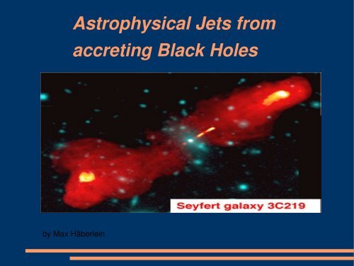
<strong>Astrophysical</strong> <strong>Jets</strong> <strong>from</strong><br />
<strong>accreting</strong> <strong>Black</strong> <strong>Holes</strong><br />
by Max Häberlein
Outline<br />
I. Description of astrophysical jets<br />
1. Sources of <strong>Jets</strong><br />
2. Formation Mechanism<br />
3. Structure of <strong>Jets</strong><br />
II. Accelaration in <strong>Jets</strong><br />
1. Fermi Acceleration<br />
2. Diffusive Shock Acceleration<br />
III. Deceleration Mechanisms<br />
1. Synchrotron Emission<br />
2. Inverse Compton Emission<br />
3. Other Processes<br />
IV. Phenomena
I.Description of astrophysical jets<br />
● <strong>Jets</strong> are a tremendous, elongated outflows of plasma<br />
● <strong>Jets</strong> can be observed in a huge spatial and energetic scale reaching<br />
<strong>from</strong> stellar size to galaxy size<br />
● There are many sources for jets<br />
● Our universe is full of jets
I.1 Sources of <strong>Jets</strong><br />
Stellar<br />
Extragalactic<br />
Object<br />
AGN<br />
GRBs<br />
Object<br />
Young Stellar Objects<br />
HMXBs<br />
LMXBs<br />
Pulsars (?)<br />
Planetary Nebulae<br />
Physical System<br />
Accreting Supermassive BH<br />
Accreting BH<br />
Physical System<br />
Accreting Star<br />
Accreting NS<br />
Accreting NS<br />
Rotating NS<br />
Accreting Nucleus or<br />
Interacting Winds
I.1 Sources of <strong>Jets</strong><br />
Active Galaxy Nuclei (AGN)<br />
● supermassive black hole in the<br />
core of a galaxy<br />
M~10 6 M Sun<br />
● there are 3 types:<br />
1. Seyfert galaxies<br />
2. Quasars<br />
3. Blazars<br />
● emits ulrarelativistic jets<br />
V escape ≃V jet ≃c ; ~3<br />
M 87
I.1 Sources of <strong>Jets</strong><br />
Microquasars<br />
● binary star system consisting<br />
of a massive normal star and a<br />
black hole bzw neutron star<br />
● timescale proportional to M<br />
> evolution of the jets within<br />
days (quasars take years)<br />
● jet velocity<br />
V escape ≃V jet ≃0.6c<br />
artists view of a microquasar
I.1 Sources of <strong>Jets</strong><br />
Gamma Ray Bursts (GRB)<br />
● flashes of gamma ray emitted<br />
by heavy stars that collapse<br />
● lifetime ~ s<br />
● followed by a longerlived<br />
afterglow<br />
● most luminous events in the<br />
sky<br />
● jet velocity<br />
V escape ≃V jet ≃c ; ~100
I.2 Structure of <strong>Jets</strong>
I.3 Formation Mechanism<br />
● not known exactly<br />
● there mainly two different<br />
theories<br />
● most popular:<br />
the magnetic field lines spin<br />
with the BH. As you go to<br />
outer regions they get faster<br />
than light. This can be handled<br />
by a nonstationary model<br />
where field lines can be<br />
twisted > jet with extreme<br />
energy
I.4 Jet Collimination
II. Acceleration in <strong>Jets</strong>
II.1 Fermi Acceleration<br />
● relativistic particle is reflected by a moving gas cloud<br />
● transformations lead to energy gain<br />
E<br />
E<br />
≈2 u<br />
c<br />
u2<br />
<br />
2<br />
c
II.2 Diffusive shock acceleration<br />
● In a uniform magnetic field a freely moving charged particle follows a<br />
helical trajectory. The particles pitch is defined as:<br />
= p⋅ B<br />
pB<br />
so its momenta are<br />
p para =p<br />
p perp =1− 2 0.5 p
II.2 Diffusive shock acceleration<br />
● What happens if a small static irregularity is imposed on the uniform<br />
field?<br />
● We are using some simplifications in the following slides<br />
1. shock normal is parallel to Bfield<br />
2. shock is planar<br />
3. we are only considering staionary solutions<br />
4. individual particle velocity v is much greater than U, the velocity of<br />
the up and downstream.
II.2 Diffusive shock acceleration<br />
● Momentum is contained because the electric field is identically zero<br />
● the pitch changes<br />
● describable in phase space by a diffusion equation, which is, considered<br />
the scattering is sufficiently stochastic, isotropic<br />
∂ f<br />
∂t<br />
=∇ ∇ f
II.2 Diffusive shock acceleration<br />
● static irregularities are unrealistic<br />
● There are two types of scattering centre motion<br />
1. largescale motions of the background which advects the scattering<br />
centres<br />
2. motion of the individual centres relative to the background (Fermi II)<br />
∂ f<br />
∂t = ∇ k ∂ f<br />
∇ f <br />
∂ t U⋅ ∇ f = ∇ k ∇ f <br />
∂<br />
∂t<br />
f x ,p=∂ f<br />
∂ x<br />
∂ x<br />
∂t<br />
U⋅ ∇ f =U⋅ ∂ f<br />
∂ x
II.2 Diffusive shock acceleration<br />
● Liuovilles theorem: phase space density has to be constant along any<br />
trajectory<br />
● for every convergence in position space you will need a divergence in<br />
momentum space<br />
∂ f<br />
∂t = ∇ k ∂ f<br />
∇ f <br />
∂ t U⋅ ∇ f = ∇ k ∇ f 1<br />
3<br />
∇⋅ U p<br />
1 1<br />
∂ f<br />
∂p
II.2 Diffusive shock acceleration<br />
● motion of the individual centres relative to the background (Fermi II)<br />
∂ f<br />
∂t = ∇ k ∂ f<br />
∇ f <br />
∂ t U⋅ ∇ f = ∇ k ∇ f 1<br />
3<br />
∇⋅ U p<br />
∂ f 1<br />
<br />
∂p p 2<br />
∂<br />
∂p p2 D<br />
1 1 2<br />
∂ f<br />
∂ p
II.2 Diffusive shock acceleration<br />
● U(x) = U1 for x < 0<br />
U(x) = U2 for x > 0<br />
⇒U<br />
∂ f ∂<br />
=<br />
∂ x ∂ x xx<br />
∂ f<br />
∂ x <br />
as a steady solution except for x =<br />
0
II.2 Diffusive shock acceleration<br />
● boundary conditions:<br />
1. x −∞⇒ f x , p f 1p<br />
2. x ∞⇒∣f x ,p∞∣<br />
3. the momentum space distribution has to be continuous<br />
4. phase space density is invariant under Lorentztransformations
II.2 Diffusive shock acceleration<br />
● 1+2 gives<br />
f x ,p~<br />
{f 1 pg 1 pexp∫ 0<br />
g 2 p= f 2 p<br />
x U dx '
II.2 Diffusive shock acceleration<br />
● The anisotropic phase space density<br />
can be expanded:<br />
where<br />
F x , p ,~ f x ,p−<br />
= v<br />
3<br />
∂ f x , p<br />
∂ x<br />
F x , p ,
II.2 Diffusive shock acceleration<br />
● Then 3+4 lead to<br />
F x , p ,~<br />
{<br />
f 1 g 1 − 3U<br />
v g 1<br />
f 2<br />
x=0 −<br />
x=0
II.2 Diffusive shock acceleration<br />
● it follows with<br />
and hence with<br />
● if a “softer” power law is incoming, a power law with slope a will<br />
come out<br />
r = U 1<br />
U 2<br />
r −1p ∂ f 2<br />
∂p =3r f 1− f 2<br />
a= 3r<br />
r −1<br />
f 2 =ap −a<br />
p<br />
∫ p '<br />
0<br />
a−1 f 1p ' dp'
II.2 Diffusive shock acceleration<br />
● From shock theorie it follows for the compression ratio<br />
r =<br />
1<br />
−1M −2<br />
that means for M ∞ and as for a nonrelativistic plasma<br />
= 5<br />
3<br />
r =4⇒a=4⇒ N x=∫ 1<br />
f x ,p'dp '~−2<br />
2<br />
4p '<br />
and for in a relativistic plasma<br />
= 4<br />
3<br />
r=7⇒ a=3.5⇒ N x=∫ 1<br />
f x ,p'dp '~−1.5<br />
2<br />
4p'
II.2 Diffusive shock acceleration<br />
● Problem: One doesnt know how the acceleration works on physical<br />
grounds<br />
● Answer: Microscopic derivation
II.2 Diffusive shock acceleration<br />
● What is the probability for a particle of escaping downstream<br />
towards ?<br />
● What is the probability of crossing the shock front?<br />
⇒<br />
∞<br />
N uptodown =∫ 0<br />
probability of not returning<br />
N esc=nU 2<br />
1<br />
v n<br />
d <br />
2 =n<br />
2<br />
nU 2<br />
nv/4 = 4U 2<br />
v<br />
v<br />
2
II.2 Diffusive shock acceleration<br />
● What is the average momentum gain when crossing the shock<br />
front?<br />
p shockfront=p1 U1 v pdownstream=p1 U 1−U 2<br />
<br />
v<br />
1<br />
〈 p〉=p∫ 0<br />
[ U 1−U 2<br />
v<br />
]2d = 2<br />
3 p U 1−U 2<br />
v
II.2 Diffusive shock acceleration<br />
● In reality p is a random variable, but for v >> U and initial<br />
momentum identically<br />
n<br />
pn~ i=1 p0[1 4<br />
3<br />
p 0<br />
U 1−U 2<br />
v i<br />
]⇒ ln pn ~<br />
p0 4<br />
3 U n<br />
1−U 2 i=1<br />
● The probability of crossing the shock front n times is<br />
n<br />
Pn~ i=11−<br />
4U 2<br />
n<br />
⇒ ln P<br />
v<br />
n~−4U 2 i=1 i<br />
⇒ P n= p −3U 2 /U 1−U 2 n<br />
=<br />
p0 p −3/r −1<br />
n<br />
<br />
p0 1<br />
v i<br />
1<br />
=−3<br />
vi U 2<br />
ln<br />
U1−U 2<br />
pn <br />
p0
II.2 Diffusive shock acceleration<br />
● With<br />
∞<br />
N x.p=∫ p<br />
N −∞ , x=<br />
4 p' 2 f x ,p 'dp'<br />
{<br />
⇒ N ∞ , x= U 1<br />
U 2<br />
0 pp 0<br />
N0 pp 0<br />
N 0<br />
pp 0
II.2 Diffusive shock acceleration<br />
● it follows<br />
f 2 p= −1<br />
4p 2<br />
N2p n=P n N p0= U1 <br />
U2 p −3/r−1<br />
n<br />
<br />
p0 ∂ N 2<br />
∂p = N 0<br />
4<br />
3U 1<br />
U 1 −U 2<br />
p<br />
−3r /r−1<br />
=<br />
p0 N −a<br />
0 p<br />
a <br />
4 p0
II.2 Diffusive shock acceleration<br />
● We again obtain a power law, but unlike other Fermi processes the<br />
slope is fixed<br />
● to verify the slope a, we can look at the synchrotron emission<br />
if the initial spectum is a power law, the synchrotron spectrum<br />
will be a power law with slope<br />
= a−1<br />
2 =0.5
II.2 Diffusive shock acceleration
III. Deceleration Mechanisms<br />
● Synchrotron Emission<br />
● Inverse Compton Scattering<br />
● proton – proton collision<br />
● Bremstrahlung<br />
X X '<br />
X X ' <br />
pp'
III.1 Synchrotron Emission<br />
● particles gyrating in the plasma field can emit photons<br />
● Synchrotron Loss Time:<br />
● Average Acceleration Time:<br />
acc = 80<br />
3<br />
sync= 6m 3<br />
p ,e c<br />
2 2<br />
T p ,e me B<br />
c<br />
2<br />
U<br />
r g<br />
b−1 r −1<br />
g, max<br />
<br />
r g
III.1 Synchrotron Emission<br />
● With acc= sync<br />
⇒ max⇒ f max =3⋅10 14 2<br />
U<br />
3b Hz<br />
2<br />
c
III.2 Inverse Compton Scattering<br />
● particles interact with the photonic background<br />
● similar as for the sychrotron emission it follows considering both<br />
effects:<br />
f max =3⋅10 14 3b U2<br />
f a Hz<br />
2<br />
c<br />
where a is the ratio of photonic to magnetic energy density
III.2 Inverse Compton Scattering
III.3 Other Processes<br />
● 1. proton – proton collision lead to a very fast<br />
deceleration<br />
2. the probability only gets dominant if the jet for example crosses a<br />
gas cloud<br />
● particles emit bremsstrahlung when they cross electric fields
IV Conclusion<br />
● My aim was<br />
1. to present a short overview about the theoretical methods used in<br />
jet physics and especially to explain fermi acceleration in a more<br />
simple way<br />
2. to show where the 2 in the power law spectrum comes <strong>from</strong><br />
3. to show that there are many things still to be done regarding jets<br />
● My aim for myself was to make a talk about theory interesting,<br />
which I found is a hard thing to do and probably will not have<br />
worked.. this time
II.2 Diffusive shock acceleration<br />
● 3+4 with p p'=p1− gives<br />
U<br />
v <br />
f 1g1= f 2<br />
U 1 p ∂<br />
∂p f 1 g 1 3U 1 g 1 =U 2 p ∂<br />
∂p f 2