New probes of initial state of quantum fluctuations during inflation
New probes of initial state of quantum fluctuations during inflation
New probes of initial state of quantum fluctuations during inflation

Create successful ePaper yourself
Turn your PDF publications into a flip-book with our unique Google optimized e-Paper software.
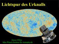
<strong>New</strong> Probes <strong>of</strong> Initial State <strong>of</strong><br />
Quantum Fluctuations <strong>during</strong><br />
Inflation<br />
Eiichiro Komatsu (Texas Cosmology Center, Univ. <strong>of</strong> Texas at Austin;<br />
Max-Planck-Institut für Astrophysik)<br />
Perimeter Institute, May 22, 2012
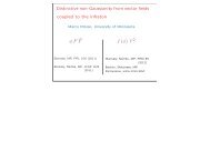
This talk is based on...<br />
• Squeezed-limit bispectrum<br />
• Ganc & Komatsu, JCAP, 12, 009 (2010)<br />
• Non-Bunch-Davies vacuum and CMB<br />
• Ganc, PRD 84, 063514 (2011)<br />
• Scale-dependent bias and μ-distortion<br />
• Ganc & Komatsu, arXiv:1204.4241 2
(Temperature Fluctuation) 2<br />
Does this plot prove <strong>inflation</strong>?<br />
=180 deg/θ<br />
3
• Can we falsify <strong>inflation</strong>?<br />
Motivation<br />
4
Falsifying “<strong>inflation</strong>”<br />
• We still need <strong>inflation</strong> to explain the flatness problem!<br />
• (Homogeneity problem can be explained by a bubble<br />
nucleation.)<br />
• However, the observed <strong>fluctuations</strong> may come from<br />
different sources.<br />
• So, what I ask is, “can we rule out <strong>inflation</strong> as a<br />
mechanism for generating the observed <strong>fluctuations</strong>?”<br />
5
First Question:<br />
• Can we falsify single-field <strong>inflation</strong>?<br />
*I will not be talking about multi-field <strong>inflation</strong> today:<br />
for potentially ruling out multi-field <strong>inflation</strong>, see<br />
Sugiyama, Komatsu & Futamase, PRL, 106, 251301 (2011)<br />
6
An Easy One: Adiabaticity<br />
• Single-field <strong>inflation</strong> = One degree <strong>of</strong> freedom.<br />
• Matter and radiation <strong>fluctuations</strong> originate from a<br />
single source.<br />
Cold<br />
Dark Matter<br />
Photon<br />
= 0<br />
* A factor <strong>of</strong> 3/4 comes from the fact that, in thermal<br />
equilibrium, ρc~ργ 3/4<br />
7
Non-adiabatic Fluctuations<br />
• Detection <strong>of</strong> non-adiabatic <strong>fluctuations</strong> immediately<br />
rule out single-field <strong>inflation</strong> models.<br />
The current CMB data are consistent with adiabatic<br />
<strong>fluctuations</strong>:<br />
| |<br />
Komatsu et al. (2011)<br />
< 0.09 (95% CL)<br />
8
Single-field <strong>inflation</strong> looks good<br />
(in 2-point function)<br />
Komatsu et al. (2011)<br />
• Pscalar(k)~k 4–ns<br />
• ns=0.968±0.012<br />
(68%CL;<br />
WMAP7+BAO+H0)<br />
• r=4Ptensor(k)/Pscalar(k)<br />
• r < 0.24 (95%CL;<br />
WMAP7+BAO+H0)<br />
9
So, let’s use 3-point function<br />
• Three-point function (bispectrum)<br />
• Bζ(k1,k2,k3)<br />
= = (amplitude) x (2π) 3 δ(k1+k2+k3)b(k1,k2,k3)<br />
k1<br />
k2<br />
k3<br />
model-dependent function<br />
10
MOST IMPORTANT, for falsifying<br />
single-field <strong>inflation</strong>
Curvature Perturbation<br />
• In the gauge where the energy density is uniform,<br />
δρ=0, the metric on super-horizon scales (k
Action<br />
• Einstein’s gravity + a canonical scalar field:<br />
•S=(1/2)∫d 4 x√–g [R–(∂Φ) 2 –2V(Φ)]<br />
13
Quantum-mechanical<br />
3 3<br />
Maldacena (2003)<br />
Computation <strong>of</strong> the Bispectrum<br />
(3)<br />
14
Initial Vacuum State<br />
ζ<br />
• Bunch-Davies vacuum, ak|0>=0 with<br />
[η: conformal time]<br />
15
Result k1<br />
Maldacena (2003)<br />
• Bζ(k1,k2,k3)<br />
= = (amplitude) x (2π) 3 δ(k1+k2+k3)b(k1,k2,k3)<br />
• b(k1,k2,k3)=<br />
x{ }<br />
Complicated? But...<br />
k2<br />
k3<br />
16
Taking the squeezed limit<br />
Maldacena (2003)<br />
• Bζ(k1,k2,k3)<br />
= = (amplitude) x (2π) 3 δ(k1+k2+k3)b(k1,k2,k3)<br />
• b(k1,k1,k3->0)=<br />
(k3
Taking the squeezed limit<br />
• b(k1,k1,k3->0)=<br />
(k3
Maldacena (2003); Seery & Lidsey (2005); Creminelli & Zaldarriaga (2004)<br />
Single-field Theorem<br />
(Consistency Relation)<br />
• For ANY single-field models * , the bispectrum in the squeezed<br />
squeezed limit (k3
Maldacena (2003); Seery & Lidsey (2005); Creminelli & Zaldarriaga (2004)<br />
Single-field Theorem<br />
(Consistency Relation)<br />
• For ANY single-field models * , the bispectrum in the squeezed<br />
squeezed limit (k3
Maldacena (2003); Seery & Lidsey (2005); Creminelli & Zaldarriaga (2004)<br />
Single-field Theorem<br />
(Consistency Relation)<br />
• For ANY single-field models * , the bispectrum in the squeezed<br />
squeezed limit (k3
Limits on fNL<br />
When fNL is independent <strong>of</strong> wavenumbers,<br />
it is called the “local type.”
Limits on fNL<br />
• fNL = 32 ± 21 (68%C.L.) from WMAP 7-year data<br />
• Planck’s CMB data is expected to yield ΔfNL=5.<br />
• fNL = 27 ± 16 (68%C.L.) from WMAP 7-year data<br />
combined with the limit from the large-scale<br />
structure (by Slosar et al. 2008)<br />
Komatsu et al. (2011)<br />
• Future large-scale structure data are expected to<br />
yield ΔfNL=1.
Understanding the Theorem<br />
• First, the squeezed triangle correlates one very longwavelength<br />
mode, kL (=k3), to two shorter wavelength<br />
modes, kS (=k1≈k2):<br />
• ≈ <br />
• Then, the question is: “why should (ζkS) 2 ever care<br />
about ζkL?”<br />
• The theorem says, “it doesn’t care, if ζk is exactly<br />
scale invariant.”<br />
24
ζkL rescales coordinates<br />
• The long-wavelength<br />
curvature perturbation<br />
rescales the spatial<br />
coordinates (or changes the<br />
expansion factor) within a<br />
given Hubble patch:<br />
• ds 2 =–dt 2 +[a(t)] 2 e 2ζ (dx) 2<br />
ζkL<br />
left the horizon already<br />
Separated by more than H -1<br />
x1=x0e ζ1 x2=x0e ζ2<br />
25
ζkL rescales coordinates<br />
• Now, let’s put small-scale<br />
perturbations in.<br />
• Q. How would the<br />
conformal rescaling <strong>of</strong><br />
coordinates change the<br />
amplitude <strong>of</strong> the small-scale<br />
perturbation?<br />
ζkL<br />
left the horizon already<br />
Separated by more than H -1<br />
(ζkS1) 2 (ζkS2) 2<br />
x1=x0e ζ1 x2=x0e ζ2<br />
26
ζkL rescales coordinates<br />
• Q. How would the<br />
conformal rescaling <strong>of</strong><br />
coordinates change the<br />
amplitude <strong>of</strong> the small-scale<br />
perturbation?<br />
• A. No change, if ζk is scaleinvariant.<br />
In this case, no<br />
correlation between ζkL and<br />
(ζkS) 2 would arise.<br />
ζkL<br />
left the horizon already<br />
Separated by more than H -1<br />
(ζkS1) 2 (ζkS2) 2<br />
x1=x0e ζ1 x2=x0e ζ2<br />
27
Creminelli & Zaldarriaga (2004); Cheung et al. (2008)<br />
Real-space Pro<strong>of</strong><br />
• The 2-point correlation function <strong>of</strong> short-wavelength<br />
modes, ξ=, within a given Hubble patch<br />
can be written in terms <strong>of</strong> its vacuum expectation value<br />
(in the absence <strong>of</strong> ζL), ξ0, as:<br />
• ξζL ≈ ξ0(|x–y|) + ζL [dξ0(|x–y|)/dζL]<br />
• ξζL ≈ ξ0(|x–y|) + ζL [dξ0(|x–y|)/dln|x–y|]<br />
• ξζL ≈ ξ0(|x–y|) + ζL (1–ns)ξ0(|x–y|)<br />
3-pt func. = = <br />
= (1–ns)ξ0(|x–y|)<br />
28<br />
• ζS(y)<br />
• ζS(x)
This is great, but...<br />
• The pro<strong>of</strong> relies on the following Taylor expansion:<br />
• ζL = 0 + ζL [d0/dζL]<br />
• Perhaps it is interesting to show this explicitly using the in-in<br />
formalism.<br />
• Such a calculation would shed light on the limitation <strong>of</strong> the<br />
above Taylor expansion.<br />
• Indeed it did - we found a non-trivial “counterexample”<br />
(more later) 29
An Idea<br />
• How can we use the in-in formalism to compute the<br />
two-point function <strong>of</strong> short modes, given that there is a<br />
long mode, ζL?<br />
• Here it is!<br />
S S<br />
ζL<br />
Ganc & Komatsu, JCAP, 12, 009 (2010)<br />
30<br />
(3)
(3)<br />
S S<br />
ζL<br />
Ganc & Komatsu, JCAP, 12, 009 (2010)<br />
Long-short Split <strong>of</strong> HI<br />
• Inserting ζ=ζL+ζS into the cubic action <strong>of</strong> a scalar<br />
field, and retain terms that have one ζL and two ζS’s.<br />
31<br />
(3)
• where<br />
Result<br />
Ganc & Komatsu, JCAP, 12, 009 (2010)<br />
32
Result<br />
• Although this expression looks nothing like (1–nS)P(k1)ζkL,<br />
we have verified that it leads to the known consistency<br />
relation for (i) slow-roll <strong>inflation</strong>, and (ii) power-law <strong>inflation</strong>.<br />
• But, there was a curious case – Alexei Starobinsky’s exact<br />
nS=1 model.<br />
• If the theorem holds, we should get a vanishing<br />
bispectrum in the squeezed limit.<br />
33
Starobinsky’s Model<br />
• The famous Mukhanov-Sasaki equation for the mode<br />
function is<br />
where<br />
•The scale-invariance results when<br />
Starobinsky (2005)<br />
So, let’s write z=B/η<br />
34
Starobinsky’s Potential<br />
• This potential is a one-parameter family; this particular<br />
example shows the case where <strong>inflation</strong> lasts very long:<br />
φend ->∞<br />
35
Result<br />
• It does not vanish!<br />
• But, it approaches zero when Φend is large, meaning the<br />
duration <strong>of</strong> <strong>inflation</strong> is very long.<br />
• In other words, this is a condition that the longest<br />
wavelength that we observe, k3, is far<br />
outside the horizon.<br />
Ganc & Komatsu, JCAP, 12, 009 (2010)<br />
• In this limit, the bispectrum approaches zero.<br />
36
Initial Vacuum State?<br />
• What we learned so far:<br />
• The squeezed-limit bispectrum is proportional to<br />
(1–nS)P(k1)P(k3), provided that ζk3 is far outside the<br />
horizon when k1 crosses the horizon.<br />
• What if the <strong>state</strong> that ζk3 sees is not a Bunch-Davies<br />
vacuum, but something else?<br />
• The exact squeezed limit (k3->0) should still obey<br />
the consistency relation, but perhaps something<br />
happens when k3/k1 is small but finite. 37
Temperature Power Spectrum<br />
How squeezed?<br />
Keisler et al. (2011)<br />
• With CMB, we can measure primordial modes in l=2–<br />
3000. Therefore, k3/k1 can be as small as 1/1500.<br />
38
Matter Power Spectrum<br />
• With large-scale structure, we can measure primordial<br />
modes in k=10 –3 –1 Mpc –1 . Therefore, k3/k1 can be as<br />
small as 1/1000.<br />
How squeezed?<br />
Hlozek et al. (2011)<br />
39
Brightness, W/m 2 /sr/Hz<br />
3m<br />
4K Black-body<br />
2.725K Black-body<br />
2K Black-body<br />
Rocket (COBRA)<br />
Satellite (COBE/FIRAS)<br />
CN Rotational Transition<br />
Ground-based<br />
Balloon-borne<br />
Satellite (COBE/DMR)<br />
30cm<br />
Using the distortion <strong>of</strong> the thermal<br />
spectrum <strong>of</strong> CMB, we can reach<br />
k3/k1 as small as 10 –8 ! (Pajer &<br />
Zaldarriaga 2012)<br />
Wavelength<br />
(plot from Samtleben et al. 2007)<br />
3mm 0.3mm<br />
40
Back to in-in<br />
• The Bunch-Davies vacuum: uk’ ~ ηe –ikη (positive frequency mode)<br />
• The integral yields 1/(k1+k2+k3) -> 1/(2k1) in the squeezed limit<br />
41
Back to in-in<br />
• Non-Bunch-Davies vacuum: uk’ ~ η(Ake –ikη + Bke +ikη negative frequency<br />
) mode<br />
• The integral yields 1/(k1–k2+k3), peaking in the folded limit<br />
• The integral yields 1/(k1–k2+k3) -> 1/(2k3) in the squeezed limit<br />
Enhanced by k1/k3: this can be a big factor!<br />
Chen et al. (2007); Holman & Tolley (2008)<br />
Agullo & Parker (2011)
ζ<br />
How about the consistency<br />
relation?<br />
k3/k1
An interesting possibility:<br />
• What if k3η0 = O(1)?<br />
• The squeezed bispectrum receives an enhancement <strong>of</strong><br />
order εk1/k3, which can be sizable.<br />
• Most importantly, the bispectrum grows faster<br />
than the local-form toward k3/k1 -> 0!<br />
• Bζ(k1,k2,k3) ~ 1/k3 3 [Local Form]<br />
• Bζ(k1,k2,k3) ~ 1/k3 4 [non-Bunch-Davies]<br />
• This has an observational consequence – particularly a<br />
scale-dependent bias and distortion <strong>of</strong> CMB spectrum.<br />
44
Power Spectrum <strong>of</strong> Galaxies<br />
• Galaxies do not trace the underlying matter density<br />
<strong>fluctuations</strong> perfectly. They are biased tracers.<br />
• “Bias” is operationally defined as<br />
• bgalaxy 2 (k) = / <br />
45
Density-ζ Relation<br />
• It is given by the Poisson equation:<br />
ζ<br />
T(k)->1 for k>10 –2 Mpc –1<br />
D(k,z)=1/(1+z) <strong>during</strong> the matter-dominated era<br />
Positive ζk -> positive δm,k!<br />
2<br />
46
Galaxy clustering modified<br />
by the squeezed limit<br />
• The existence <strong>of</strong> long-wavelength ζ changes the smallscale<br />
power <strong>of</strong> δm.<br />
• A positive long-wavelength ζ -> more power<br />
on small scales.<br />
• More power on small scales -> more galaxies formed.<br />
47
Dalal et al. (2008); Matarrese & Verde (2008); Desjacques et al. (2011)<br />
Scale-dependent Bias<br />
• A rule-<strong>of</strong>-thumb:<br />
• For B(k1,k2,k3) ~ 1/k3 p , the scale-dependence <strong>of</strong> the<br />
halo bias is given by b(k) ~ 1/k p–1<br />
• For a local-form (p=3), it goes like b(k)~1/k 2<br />
• For a non-Bunch-Davies vacuum (p=4), would it go like<br />
b(k)~1/k 3 ?<br />
MR(k)~k 2 for k1/R<br />
R is the linear size<br />
<strong>of</strong> dark matter halos<br />
48
Δbgalaxy(k)/bgalaxy<br />
~k –2<br />
Local<br />
(fNL=10)<br />
~k –3<br />
It does! Ganc & Komatsu (2012)<br />
non-BD<br />
vacuum<br />
(ε=0.01; Nk=1)<br />
Wavenumber, k [h Mpc –1 ]<br />
49
Ganc, PRD 84, 063514 (2011); Ganc & Komatsu (2012)<br />
CMB Bispectrum<br />
• The expected contribution to fNL as measured by the<br />
CMB bispectrum is typically fNL≈8(ε/0.01).<br />
• A lot bigger than (5/12)(1–nS), and could be<br />
detectable with Planck.<br />
• Note that this does not mean a violation <strong>of</strong> the singlefield<br />
consistency condition, which is valid in the exact<br />
squeezed limit, k3->0.<br />
• We have an enhanced bispectrum in the squeezed<br />
configuration where k3/k1 is small but finite.<br />
50
Brightness, W/m 2 /sr/Hz<br />
3m<br />
4K Black-body<br />
2.725K Black-body<br />
2K Black-body<br />
Rocket (COBRA)<br />
Satellite (COBE/FIRAS)<br />
CN Rotational Transition<br />
Ground-based<br />
Balloon-borne<br />
Satellite (COBE/DMR)<br />
30cm<br />
Using the distortion <strong>of</strong> the thermal<br />
spectrum <strong>of</strong> CMB, we can reach<br />
k3/k1 as small as 10 –8 ! (Pajer &<br />
Zaldarriaga 2012)<br />
Wavelength<br />
(plot from Samtleben et al. 2007)<br />
3mm 0.3mm<br />
51
Temperature Power Spectrum<br />
Damping <strong>of</strong> Acoustic Waves<br />
• Energy stored in the acoustic waves must go<br />
somewhere -> heating <strong>of</strong> CMB photons -> distortion <strong>of</strong><br />
the thermal spectrum<br />
Exponential<br />
Damping<br />
52
Chemical potential from<br />
energy injection<br />
• Suppose that some energy, ΔE, is injected into the<br />
cosmic plasma <strong>during</strong> the radiation dominated era.<br />
• What happens? The thermal spectrum <strong>of</strong> CMB should<br />
be distorted!<br />
53
Chemical potential from<br />
energy injection<br />
• For z>zi=2x10 6 , double Compton scattering, e – +γ->e –<br />
+2γ, is effective, erasing the distortion <strong>of</strong> the thermal<br />
spectrum <strong>of</strong> CMB.<br />
• Black-body spectrum is restored.<br />
54
Chemical potential from<br />
energy injection<br />
• For ze –<br />
+2γ, freezes out.<br />
• However, the elastic scattering, e – +γ->e – +γ, remains<br />
effective [until zf=5x10 4 ]<br />
• Black-body spectrum is not restored, but the spectrum<br />
relaxes to a Bose-Einstein spectrum with a non-zero<br />
chemical potential, μ, for zf
Chemical potential from<br />
n(ν)=<br />
energy injection<br />
• Energy density is added to the plasma (μ
How much energy?<br />
• Only 1/3 <strong>of</strong> the total energy stored in the acoustic<br />
wave <strong>during</strong> radiation era is used to heat CMB (thus<br />
distorting the CMB spectrum) (papers by Jens Chluba):<br />
• Q = (1/3)(9/4)cs 2 ργ(δγ) 2 = (1/4)ργ(δγ) 2<br />
• μ≈1.4∫dz[(dQ/dz)/ργ]<br />
=(1.4/4)[(δγ) 2 (zi)–(δγ) 2 (zf)]<br />
• where zi=2x10 6 and zf=5x10 4<br />
57
Bottom Line<br />
• Therefore, the chemical potential is generated by<br />
the photon density perturbation squared.<br />
• At what scale? The diffusion damping occurs at<br />
the mean free path <strong>of</strong> photons. In terms <strong>of</strong> the<br />
wavenumber, it is given by:<br />
It’s a very small scale!<br />
(compared to the large-scale structure, k~1 Mpc –1 )<br />
;<br />
58
μ-distortion modified by<br />
the squeezed limit<br />
• The existence <strong>of</strong> long-wavelength ζ changes the smallscale<br />
power <strong>of</strong> δγ.<br />
• A positive long-wavelength ζ -> more power<br />
on small scales.<br />
• More power on small scales -> more μ-distortion.<br />
• μ-distortion becomes anisotropic on the<br />
sky! (Pajer & Zaldarriaga 2012) 59
μ-T cross-correlation<br />
• In real space:<br />
• μ = (1.4/4)[(δγ) 2 (zi)–(δγ) 2 (zf)] at k1~O(10 2 )–O(10 4 )<br />
• ΔT/T = –(1/5)ζ at k3~O(10 –4 ) [in the Sachs-Wolfe<br />
limit]<br />
• Correlating these will probe the bispectrum in the<br />
squeezed configuration with k3/k1=O(10 –6 )–O(10 –8 )!!<br />
60
More exact treatment<br />
• Going to harmonic space:<br />
• ΔT/T(n)=∑alm T Ylm(n); μ(n)=∑alm μ Ylm(n)<br />
•<br />
•<br />
[gTl(k) contains info about<br />
the acoustic oscillation]<br />
61
Pajer & Zaldarriaga (2012); Ganc & Komatsu (2012)<br />
μ-T cross-power spectrum<br />
• Here, the integral is dominated by k1≈k2≈kD (which is<br />
big) and k≈l/rL (which is small because rL=14000 Mpc)<br />
• Very squeezed limit bispectrum<br />
62
μ-T cross-correlation<br />
Local-form Result<br />
Ganc & Komatsu (2012)<br />
Full calculation (our result)<br />
[sign changes]<br />
Sachs-Wolfe approximation (Pajer&Zaldarriaga)<br />
[always negative]<br />
63
Signal-to-noise / fNL<br />
Can we detect the local-<br />
form bispectrum?<br />
Ganc & Komatsu (2012)<br />
Sachs-Wolfe approximation<br />
Full calculation (infinite resolution)<br />
Full calculation (PIXIE’s resolution)<br />
• No, unless fNL>>2300<br />
64
Signal-to-noise<br />
But, a modified <strong>initial</strong> <strong>state</strong><br />
enhances the signal<br />
maximum signal<br />
more realistic estimate<br />
Occupation Number (=|βk| 2 )<br />
Ganc & Komatsu (2012)<br />
65<br />
60!
Future Work<br />
• All we did was to impose the following mode function<br />
at a finite past:<br />
• uk = [αk(1+ikη)e –ikη + βk(1–ikη)e ikη ]<br />
• with the condition: βk -> 0 for k->∞<br />
• However, it is desirable to construct an explicit model<br />
which will give explicit forms <strong>of</strong> αk and βk, so that we<br />
do not need to put an arbitrary model function at an<br />
arbitrary time by hand.<br />
66
<strong>New</strong> <strong>probes</strong> <strong>of</strong> <strong>initial</strong> <strong>state</strong><br />
<strong>of</strong> <strong>quantum</strong> <strong>fluctuations</strong>!<br />
{<br />
Summary<br />
• A more insight into the single-field consistency relation<br />
for the squeezed-limit bispectrum using in-in formalism.<br />
• Non-Bunch-Davies vacuum can give an enhanced<br />
bispectrum in the k3/k1