Analytic Hypersonic Aerodynamics for Conceptual Design of Entry ...

This allows the limits of integration in v to be defined by the solution of sin(θ) = 0. If the shape was not
convex, then shadowed regions may have boundaries where sin(θ) = 0.
Step 4: Compute Reference Values
The reference area and reference length for each shape is computed based on the parametrization used. The
reference area is computed as the projected area of the shape on the y-z plane using Eq. (13) assuming
α = β = 0, where dAplanar is the incremental area projected on the y-z plane. Since ru × rv represents the
inward normal of a convex shape and dAplanar must be positive to obtain a positive reference area, dAplanar
is computed using Eq. (14). Due to the convexity requirement of the shape, the entire surface is unshadowed
at α = β = 0, and, consequently, the limits of integration must be chosen to span the entire surface of the
shape. The reference length is computed as the maximum span of the vehicle in the x-direction.
Step 5: Evaluate Surface Integral
Aref =
umax vmax
umin
vmin
dAplanar
(13)
dAplanar = (ru × rv) T (−ˆx) (14)
The aerodynamic coefficients are computed by evaluating the surface integral in Eq. (4) and Eq. (5). The
first integration is performed with respect to v since the shadow boundary was solved as v = v(u). After the
integration is performed with respect to v, the shadow boundaries are substituted as the limits of integration
for v. The remaining integrand is only a function of u, and the second integration is performed with respect
to u. The limits of integration substituted for u are constants, u1 and u2. During evaluation of the analytic
expressions, the designer specifies the portion of the shape used by supplying the values for u1 and u2.
Step 6: Output Aerodynamics Code
After the analytic relations have been developed, they are output to a Matlab-based aerodynamics module.
This module contains the analytic relations, reference area, and reference length. Hence, as the analytic
relations of various shapes are developed, the aerodynamics module becomes a library containing analytic
relations for a wide variety of shapes.
V. Derivation and Validation of Analytic Expressions for Basic Shapes
The shape of common entry vehicles can be constructed via the superposition of basic shapes. The
construction and parametrization of the various basic shapes will be shown. It is important to note that all
basic shapes are parametrized by variables describing the family of the basic shape, such as the half-angle of
a sharp cone, and by variables describing the surface, u and v, as previously described. This generalization
of each basic shape allows the development of only one set of analytic relations for each basic shape family.
Each basic shape is chosen to have symmetry along the body axes where applicable and be centered at the
origin. A range of angles of attack and sideslip was chosen to validate both shadowed and unshadowed angles
of attack.
V.A. Sharp Cone Family
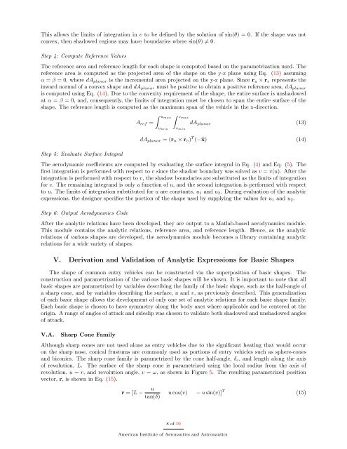
Although sharp cones are not used alone as entry vehicles due to the significant heating that would occur
on the sharp nose, conical frustums are commonly used as portions of entry vehicles such as sphere-cones
and biconics. The sharp cone family is parametrized by the cone half-angle, δc, and length along the axis
of revolution, L. The surface of the sharp cone is parametrized using the local radius from the axis of
revolution, u = r, and revolution angle, v = ω, as shown in Figure 5. The resulting parametrized position
vector, r, is shown in Eq. (15).
r = [L − u
tan(δ)
u cos(v) − u sin(v)] T
8 of 19
American Institute of Aeronautics and Astronautics
(15)