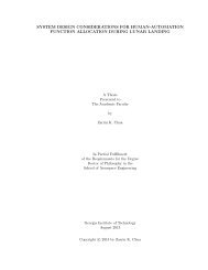
Thermal, Structural, and Inflation Modeling of an Isotensoid ...
Thermal, Structural, and Inflation Modeling of an Isotensoid ...
Thermal, Structural, and Inflation Modeling of an Isotensoid ...

You also want an ePaper? Increase the reach of your titles
YUMPU automatically turns print PDFs into web optimized ePapers that Google loves.
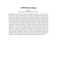
<strong>Thermal</strong>, <strong>Structural</strong>, <strong><strong>an</strong>d</strong> <strong>Inflation</strong> <strong>Modeling</strong> <strong>of</strong> <strong>an</strong><br />
<strong>Isotensoid</strong> Supersonic Inflatable Aerodynamic Decelerator<br />
Br<strong><strong>an</strong>d</strong>on P. Smith, I<strong>an</strong> G. Clark, <strong><strong>an</strong>d</strong> Robert D. Braun<br />
D<strong>an</strong>iel Guggenheim School <strong>of</strong> Aerospace Engineering<br />
Georgia Institute <strong>of</strong> Technology<br />
270 Ferst Drive<br />
Atl<strong>an</strong>ta, GA 30332-0150<br />
404-894-7783<br />
bpsmith@gatech.edu<br />
Abstract—Near-term missions to Mars may not be possible<br />
with current deployable decelerator technology. This<br />
possibility becomes a certainty for the more dist<strong>an</strong>t hum<strong>an</strong>precursor<br />
missions. Inflatable Aerodynamic Decelerators<br />
(IADs) are a c<strong><strong>an</strong>d</strong>idate technology that may provide the<br />
needed drag augmentation to enable these much heavier<br />
missions. The attached isotensoid is one <strong>of</strong> the IAD<br />
configurations favored for application at Mars. Assessing<br />
the isotensoid’s technical feasibility for Mars missions<br />
requires several perform<strong>an</strong>ce models capable <strong>of</strong> providing<br />
reasonably accurate predictions <strong>of</strong> key design parameters.<br />
This paper describes engineering-level models derived from<br />
past isotensoid technology development efforts that have<br />
been modified or improved for the problem at h<strong><strong>an</strong>d</strong>. Easily<br />
implemented models <strong>of</strong> the isotensoid inflation history,<br />
aerothermodynamic environment, <strong><strong>an</strong>d</strong> thermostructural<br />
perform<strong>an</strong>ce are described. 1 2<br />
Engineering models are presented for estimating internal<br />
pressure <strong><strong>an</strong>d</strong> drag during inflation, aerothermal heating on<br />
the fabric, stresses throughout the structure, <strong><strong>an</strong>d</strong> in-depth<br />
fabric temperatures. The models are applied to a reference<br />
mission similar to the Mars Science Laboratory (MSL)<br />
employing a Supersonic IAD (SIAD) at Mach 5.<br />
Thermostructural <strong>an</strong>alysis is presented to show a method for<br />
selecting suitable materials capable <strong>of</strong> performing in the<br />
predicted aerothermal environment under the predicted load.<br />
The inflation model is validated with empirical data from<br />
Viking-era ground tests. Aerothermal <strong>an</strong>alysis shows that a<br />
peak convective heat rate <strong>of</strong> 1.25 W/cm 2 c<strong>an</strong> be expected<br />
across the isotensoid fabric. Stresses are computed for<br />
minimum gauge materials, <strong><strong>an</strong>d</strong> the tr<strong>an</strong>sient temperature<br />
response <strong>of</strong> the fabric <strong><strong>an</strong>d</strong> thermal coating is computed.<br />
Nomex, Kevlar, <strong><strong>an</strong>d</strong> Vectr<strong>an</strong> materials are considered.<br />
Material tenacity retention at elevated temperatures is<br />
considered. Vectr<strong>an</strong> is recommended for the isotensoid<br />
fabric due to its adequate thermostructural perform<strong>an</strong>ce,<br />
favorable abrasive properties, <strong><strong>an</strong>d</strong> flight heritage as <strong>an</strong><br />
inflatable structure.<br />
1 978-1-4244-7351-9/11/$26.00 ©2011 IEEE.<br />
2 IEEEAC paper #1312, Version 4, Updated J<strong>an</strong>uary 10, 2011<br />
1<br />
TABLE OF CONTENTS<br />
1. INTRODUCTION ............................................................ 1 <br />
2. REFERENCE MISSION ................................................... 2 <br />
3. INFLATION MODEL ...................................................... 2 <br />
4. AEROTHERMAL MODEL AND ANALYSIS ..................... 6 <br />
5. THERMAL MODEL ........................................................ 8 <br />
6. CANDIDATE MATERIALS ........................................... 10 <br />
7. THERMOSTRUCTURAL ANALYSIS .............................. 11 <br />
8. CONCLUSION .............................................................. 14 <br />
REFERENCES ....................................................................... 14 <br />
BIOGRAPHY ........................................................................ 15 <br />
1. INTRODUCTION<br />
Inflatable Aerodynamic Decelerators (IADs) are a<br />
promising technology for greatly increasing perform<strong>an</strong>ce <strong>of</strong><br />
entry probes at Mars <strong><strong>an</strong>d</strong> other pl<strong>an</strong>etary atmospheres.<br />
NASA <strong><strong>an</strong>d</strong> the Department <strong>of</strong> Defense have been the main<br />
proprietors <strong>of</strong> this technology through a sporadic<br />
development history sp<strong>an</strong>ning fifty years. The technology<br />
reached a pinnacle during the mission pl<strong>an</strong>ning phases <strong>of</strong><br />
the Viking, Pioneer Venus, <strong><strong>an</strong>d</strong> Galileo missions, <strong><strong>an</strong>d</strong><br />
modern efforts have focused on building on this extensive<br />
historical knowledge base [1]. IADs have proven technical<br />
feasibility far beyond the proven flight envelope <strong>of</strong> the diskgap-b<strong><strong>an</strong>d</strong><br />
parachute, but they have never been tested in a<br />
relev<strong>an</strong>t environment at their intended scale. The attached<br />
isotensoid Supersonic Inflatable Aerodynamic Decelerator<br />
(SIAD) is one <strong>of</strong> the favored configurations for high-mass<br />
missions to Mars. This geometry consists <strong>of</strong> <strong>an</strong> inflatable<br />
textile envelope designed for uniform fabric stress in both<br />
principle directions <strong><strong>an</strong>d</strong> is augmented with meridional cords<br />
for fabric load relief. NASA, industry, <strong><strong>an</strong>d</strong> academia are<br />
currently developing test <strong><strong>an</strong>d</strong> <strong>an</strong>alysis techniques to mature<br />
this <strong><strong>an</strong>d</strong> other IAD configurations.<br />
The flexible nature <strong>of</strong> inflatable structures <strong><strong>an</strong>d</strong> the extreme<br />
operating environment make high-fidelity perform<strong>an</strong>ce<br />
<strong>an</strong>alysis difficult during preliminary design. This paper<br />
builds on previous literature by presenting simple methods<br />
for computing several useful engineering qu<strong>an</strong>tities for<br />
<strong>an</strong>alysis <strong>of</strong> attached isotensoids: drag <strong><strong>an</strong>d</strong> internal pressure<br />
histories during inflation, aerothermodynamic heating on the<br />
isotensoid fabric, peak fabric <strong><strong>an</strong>d</strong> cord stresses, <strong><strong>an</strong>d</strong> fabric<br />
temperature pr<strong>of</strong>iles. The models are described in detail <strong><strong>an</strong>d</strong><br />
validated using <strong>an</strong>alytic methods or experimental data where<br />
available.
Presented models are applied to a reference mission similar<br />
to the Mars Science Laboratory (MSL). The results are<br />
estimates <strong>of</strong> key qu<strong>an</strong>tities that must be known early in the<br />
design process for purposes <strong>of</strong> evaluating feasibility <strong>of</strong><br />
SIAD configurations, identifying import<strong>an</strong>t sensitivities,<br />
<strong><strong>an</strong>d</strong> informing design <strong>of</strong> ground <strong><strong>an</strong>d</strong> flight tests. One<br />
historical material (Nomex) <strong><strong>an</strong>d</strong> two modern materials<br />
(Kevlar <strong><strong>an</strong>d</strong> Vectr<strong>an</strong>) are considered for the SIAD structure.<br />
Design recommendations are made based on the<br />
thermostructural results <strong><strong>an</strong>d</strong> packaging considerations.<br />
2. REFERENCE MISSION<br />
This <strong>an</strong>alysis considers the atmospheric deceleration <strong>of</strong> a<br />
blunt-body aeroshell with <strong>an</strong> attached isotensoid SIAD. The<br />
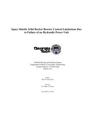
attached isotensoid, shown notionally in Figure 1, is one <strong>of</strong><br />
the SIAD configurations being studied for atmospheric<br />
deceleration within the pl<strong>an</strong>etary exploration community.<br />
The isotensoid geometry is characterized by a fabric<br />
envelope attached to the rigid aeroshell at shoulder <strong><strong>an</strong>d</strong><br />
backshell locations. Ram-air inlets located on the fabric<br />
envelope provide the required inflation gas. Some isotensoid<br />
configurations include <strong>an</strong> extra “burble fence” located at the<br />
SIAD shoulder. This feature provides uniform flow<br />
separation <strong><strong>an</strong>d</strong> must be included for stable subsonic flight.<br />
Inlets<br />
Burble Fence<br />
Figure 1 – Attached isotensoid SIAD.<br />
System studies show that SIADs provide the most trajectory<br />
benefits at Mars when deployed at Mach 4-6 between 10<br />
<strong><strong>an</strong>d</strong> 20 km [2]. This <strong>an</strong>alysis considers a nominal SIAD<br />
deployment at Mach 5. The assumed deployment dynamic<br />
pressure <strong>of</strong> 4 kPa is conservative for this r<strong>an</strong>ge <strong>of</strong> altitudes.<br />
A cross-sectional view <strong>of</strong> the aeroshell <strong><strong>an</strong>d</strong> deployed SIAD<br />
is shown in Figure 2 with coordinates <strong>of</strong> the identified<br />
locations listed in Table 1. The isotensoid is sized to provide<br />
approximately four times the supersonic drag area, C D A, <strong>of</strong><br />
the MSL aeroshell, or 105 m 2 . This yields <strong>an</strong> attached<br />
isotensoid with a diameter <strong>of</strong> 11 m.<br />
Table 1 – Coordinates <strong>of</strong> attached isotensoid features.<br />
Point Definition Radial<br />
(m)<br />
Axial<br />
(m)<br />
A Front Attachment Point 2.21 0.0250<br />
B Maximum <strong>Isotensoid</strong> Radius 5.00 2.83<br />
C Maximum Total Radius 5.50 3.08<br />
D Burble Fence Origin 5.00 3.08<br />
E Maximum Height 3.57 4.10<br />
F Rear Attachment Point 2.10 0.308<br />
G Centroid <strong>of</strong> SIAD 3.28 2.30<br />
H Inlet Attachment Point 4.25 1.34<br />
Axial, m<br />
4<br />
3.5<br />
3<br />
2.5<br />
2<br />
1.5<br />
1<br />
0.5<br />
0<br />
!0.5<br />
Aeroshell<br />
F<br />
SIAD<br />
A<br />
0 1 2 3 4 5 6<br />
Radial, m<br />
Figure 2 – Pr<strong>of</strong>ile <strong>of</strong> aeroshell with supersonic attached<br />
isotensoid (coordinates provided in Table 1).<br />
3. INFLATION MODEL<br />
This section provides a description <strong>of</strong> a mathematical model<br />
for predicting the inflation <strong>of</strong> <strong>an</strong> attached isotensoid SIAD.<br />
Specifically, the model provides a me<strong>an</strong>s for estimating the<br />
rate <strong>of</strong> inflation <strong>of</strong> <strong>an</strong> isotensoid employing ram-air inlets in<br />
terms <strong>of</strong> the rate <strong>of</strong> internal pressure <strong><strong>an</strong>d</strong> drag area increase.<br />
These relations are needed for evaluating the trajectory<br />
implications <strong>of</strong> SIAD deployment <strong><strong>an</strong>d</strong> computing the design<br />
stresses in the isotensoid materials. Primary inputs to the<br />
model include the freestream conditions, volume <strong>of</strong> the<br />
SIAD, <strong><strong>an</strong>d</strong> area <strong>of</strong> the ram-air inlets. The model builds on<br />
prior inflation models available in the literature [3][4] <strong><strong>an</strong>d</strong><br />
relies predomin<strong>an</strong>tly on isentropic flow relations.<br />
The process <strong>of</strong> isotensoid inflation is broken into three main<br />
phases (inlet deployment, volume rise, <strong><strong>an</strong>d</strong> pressure rise)<br />
delineated by four events. The events are as follows:<br />
Start <strong>of</strong> <strong>Inflation</strong>, t 0 : This marks the initiation <strong>of</strong> the<br />
inflation process. At this time the isotensoid is pushed out<br />
from where it is stored <strong><strong>an</strong>d</strong> the fabric is exposed to the<br />
freestream. The event would likely be represented by the<br />
firing <strong>of</strong> a small gas generator <strong><strong>an</strong>d</strong> the separation <strong>of</strong> <strong>an</strong>y<br />
cover p<strong>an</strong>els used to protect the SIAD during entry. The gas<br />
generator is used to provide a small initial pressurization <strong>of</strong><br />
the SIAD that would be sufficient to expose the ram-air<br />
inlets to the oncoming flow.<br />
Inlets in Freestream, t if : At this point the ram-air inlets are<br />
exposed to the freestream <strong><strong>an</strong>d</strong> the SIAD begins inflating in<br />
earnest. Early on in the inflation process the SIAD has<br />
insufficient internal pressure to overcome freestream forces<br />
<strong><strong>an</strong>d</strong> thus the isotensoid begins to inflate aft <strong>of</strong> the entry<br />
vehicle. This inflation process takes the form <strong>of</strong> a const<strong>an</strong>t<br />
pressure process in which ingested air is used to strictly<br />
raise the volume <strong>of</strong> the SIAD. Because the SIAD is<br />
exp<strong><strong>an</strong>d</strong>ing into the aft region <strong>of</strong> the entry vehicle, the<br />
G<br />
E<br />
H<br />
D<br />
B<br />
C<br />
2
!<br />
internal pressure is assumed to be equal to the base pressure,<br />
P b .<br />
Full Volume, t fv : At this point the SIAD has exp<strong><strong>an</strong>d</strong>ed as<br />
much into the aft regions <strong>of</strong> the entry vehicle as possible<br />
without extending past the shoulder <strong>of</strong> the vehicle. For<br />
modeling purposes, it is assumed that the SIAD has<br />
achieved a volume the same as the fully deployed volume.<br />
This marks the end <strong>of</strong> the const<strong>an</strong>t pressure phase <strong>of</strong><br />
inflation <strong><strong>an</strong>d</strong> subsequently air ingested is used to begin<br />
increasing the pressure so as to push the SIAD out beyond<br />
the shoulders <strong>of</strong> the entry vehicle.<br />
Full Pressure, t fp : <strong>Inflation</strong> is assumed to end once the<br />
SIAD has reached 99% <strong>of</strong> the maximum inflation pressure<br />
value (either the freestream stagnation pressure or the<br />
stagnation pressure behind a normal shock).<br />
Internal Pressure Model<br />
The internal pressure model begins once the inlets are<br />
exposed to the freestream, at time t if . The internal pressure<br />
<strong>of</strong> the isotensoid is governed by the mass flow rate into the<br />
SIAD via the ram-air inlets <strong><strong>an</strong>d</strong> the mass flow rate out <strong>of</strong> the<br />
SIAD due to the porosity <strong>of</strong> the c<strong>an</strong>opy. Calculations <strong>of</strong><br />
both flow rates are dependent on whether the flow is<br />
choked.<br />
Freestream Calculations—Several parameters dependent on<br />
the freestream conditions are required for subsequent<br />
calculations. Equations for these are as follows:<br />
!<br />
$ # +1<br />
P 02<br />
= P "<br />
! 2 M 2 '<br />
"<br />
%<br />
&<br />
(<br />
)<br />
%<br />
T 0 = T " 1+ # $1<br />
2 M 2 (<br />
"<br />
&<br />
'<br />
)<br />
* (1)<br />
%<br />
P 01<br />
= P " 1+ # $1<br />
2 M " 2 (<br />
&<br />
'<br />
)<br />
*<br />
# (# *1)<br />
# (# $1)<br />
1<br />
$<br />
# +1<br />
'<br />
(# *1)<br />
&<br />
)<br />
%&<br />
2#M 2 " * (# *1)<br />
()<br />
where Equation (1) defines the freestream stagnation<br />
!<br />
temperature, T 0 , Equation (2) defines the freestream<br />
stagnation pressure, P 01 , <strong><strong>an</strong>d</strong> Equation (3) defines the<br />
stagnation pressure behind a normal shock, P 02 . T ∞ is the<br />
freestream static temperature, P ∞ is the freestream static<br />
pressure, M ∞ is the freestream Mach number, <strong><strong>an</strong>d</strong> γ is<br />
specific heat ratio at Mars (γ ≈1.3). Note that Equation (3) is<br />
only valid for flight Mach numbers greater th<strong>an</strong> one. For<br />
Mach numbers less th<strong>an</strong> one, Equation 4 below should be<br />
used for the value <strong>of</strong> P 02 . The reason for this is that in later<br />
calculations, P 02 will be used as the value <strong>of</strong> the maximum<br />
internal pressure.<br />
The pressure at the base <strong>of</strong> the isotensoid, P b , is calculated<br />
using <strong>an</strong> empirical relation [3] as follows:<br />
!<br />
(2)<br />
(3)<br />
P 02<br />
= P 01<br />
(4)<br />
3<br />
C pb<br />
=<br />
"1<br />
M # 2 + 0.7<br />
$ 1 '<br />
P b<br />
= P #<br />
"&<br />
) * % M 2 #<br />
+ 0.7(<br />
2 P 2<br />
#M #<br />
where C pb is the base pressure coefficient. Note that<br />
Equation (5) is based on supersonic flow. However, <strong>an</strong><br />
examination ! <strong>of</strong> data from recent tr<strong>an</strong>sonic testing <strong>of</strong> blunt<br />
bodies indicates that the equation c<strong>an</strong> be useful at lower<br />
Mach numbers so long as a lower bound <strong>of</strong> C pb ~ -0.4 is<br />
enforced. Prior codes have needed to use a const<strong>an</strong>t value <strong>of</strong><br />
base pressure due to numerical stability issues. However,<br />
this depends on the numerical methods used. Keeping the<br />
value const<strong>an</strong>t is not thought to be <strong>an</strong> issue because the<br />
value does not ch<strong>an</strong>ge very quickly with Mach number <strong><strong>an</strong>d</strong><br />
furthermore the Mach number is unlikely to ch<strong>an</strong>ge<br />
signific<strong>an</strong>tly during a typical inflation.<br />
Inlet Flow Rate—Calculating the mass flow rate into the<br />
isotensoid, !m i<br />
, via the ram-air inlets requires first<br />
determining if the flow is choked at the inlet. Thus, two<br />
relations are required with a conditional statement as<br />
follows:<br />
if<br />
( )<br />
P i<br />
%<br />
" 1+ # $1 (<br />
# 1$#<br />
' *<br />
P 02<br />
& 2 )<br />
,<br />
. # % 2 (<br />
m ˙ i = C d i<br />
+ i A i P 02 . ' *<br />
RT 0 &# +1)<br />
-.<br />
else<br />
, %<br />
. # '%<br />
m ˙ i = C d i<br />
+ i A i P 02 . '<br />
RT '<br />
. 0 '&<br />
- &<br />
P i<br />
P 02<br />
# +1<br />
1 2<br />
/<br />
# $1<br />
2<br />
1<br />
1<br />
01<br />
(# %<br />
P<br />
(<br />
* $ i<br />
'<br />
) & P *<br />
02 )<br />
# +1<br />
#<br />
where P i is the static inlet pressure, A i is the inlet area, <strong><strong>an</strong>d</strong> R<br />
is the gas const<strong>an</strong>t. The conditional statement evaluates the<br />
total pressure ratio at the inlet to determine if the flow is<br />
choked. A slight improvement to the conditional statement<br />
would be to use the local static pressure upstream <strong>of</strong> the<br />
inlet, rather th<strong>an</strong> the total pressure. The current formulation<br />
assumes that the inlets are located far enough forward to the<br />
nose <strong>of</strong> the vehicle that the two pressures are reasonably<br />
close.<br />
The mass flow rate is assumed to be proportional to the<br />
isentropic flow rate, where the const<strong>an</strong>t <strong>of</strong> proportionality is<br />
the product <strong>of</strong> the inlet efficiency parameter, η i , <strong><strong>an</strong>d</strong> the<br />
discharge coefficient, C di . For the inlets, the value <strong>of</strong> the<br />
discharge coefficient is taken to be that <strong>of</strong> a sharp-edged<br />
orifice, for which a curve fit was made from data available<br />
in Reference [5]. The curve fit is as follows:<br />
(/<br />
* 1<br />
* 1<br />
* 1<br />
) 0<br />
1 2<br />
(5)<br />
(6)
!<br />
!<br />
!<br />
C d i<br />
3<br />
"<br />
= 0.4861 P % "<br />
i<br />
$<br />
# P '<br />
( 0.8274 P % "<br />
i<br />
$<br />
02 & # P '<br />
+ .0992 P %<br />
i<br />
$<br />
02 & # P ' + 0.85 (7)<br />
02 &<br />
The inlet efficiency parameter is a function <strong>of</strong> how the inlet<br />
is made <strong><strong>an</strong>d</strong> what the shape is. From Reference [6], <strong>an</strong> η i<br />
value <strong>of</strong> 0.7 is recommended for a cloth inlet like that used<br />
for <strong>an</strong> attached isotensoid.<br />
C<strong>an</strong>opy Porosity Flow Rate—Calculating the mass flow rate<br />
out <strong>of</strong> the c<strong>an</strong>opy due to porosity, !m o<br />
, is performed in a<br />
m<strong>an</strong>ner similar to that for the inlets, though without the inlet<br />
efficiency parameter.<br />
if P %<br />
b<br />
" 1+ # $1 (<br />
# ( 1$# )<br />
' *<br />
P i & 2 )<br />
+<br />
m ˙<br />
- # % 2 (<br />
o = C d o<br />
A base P i - ' *<br />
RT 0 &# +1)<br />
,-<br />
else<br />
+ %<br />
- # '%<br />
m ˙ o = C d o<br />
A base P i - '<br />
RT - 0 '&<br />
, &<br />
P b<br />
P i<br />
2<br />
# +1<br />
1 2<br />
.<br />
# $1<br />
2<br />
0<br />
0<br />
/ 0<br />
(# % P (<br />
* $ ' b<br />
*<br />
) & )<br />
P i<br />
# +1<br />
#<br />
where A base is the surface area <strong>of</strong> fabric located in the SIAD<br />
base. The discharge coefficient in Equation 8 is a function<br />
<strong>of</strong> the porosity <strong>of</strong> the material <strong><strong>an</strong>d</strong> the pressure differential<br />
between the internal pressure <strong><strong>an</strong>d</strong> the base pressure <strong>of</strong> the<br />
SIAD. Values <strong>of</strong> the discharge coefficient will be dependent<br />
on the type <strong>of</strong> material used <strong><strong>an</strong>d</strong> the degree to which the<br />
material was made non-porous (e.g. through coating or<br />
calendaring). To provide insight into a r<strong>an</strong>ge <strong>of</strong> values<br />
typical for <strong>an</strong> isotensoid, data was extracted from Reference<br />
[7] for the permeability <strong>of</strong> <strong>an</strong> isotensoid model at a r<strong>an</strong>ge <strong>of</strong><br />
differential pressures. The data is originally provided as a<br />
measure <strong>of</strong> permeability in units <strong>of</strong> ft 3 /min/ft 2 across a r<strong>an</strong>ge<br />
<strong>of</strong> pressures <strong><strong>an</strong>d</strong> fabric coating levels. Using information in<br />
the Reference, a value <strong>of</strong> the discharge coefficient was<br />
backed out using Equation (8) <strong><strong>an</strong>d</strong> is shown plotted in<br />
Figure 3. The data was fitted using <strong>an</strong> equation <strong>of</strong> the<br />
following form:<br />
C d o<br />
= aexp b( P i<br />
" P b )<br />
(.<br />
* 0<br />
0<br />
*<br />
)<br />
0<br />
/<br />
1 2<br />
(8)<br />
[ ] + c exp[ d( P i<br />
" P b )] (9)<br />
Values <strong>of</strong> the coefficients for each <strong>of</strong> the three vari<strong>an</strong>ts <strong>of</strong><br />
models tested are provided in Table 2. It is worth noting that<br />
none <strong>of</strong> the intercepts for the curve fits passes through zero<br />
for a zero pressure differential. This is considered <strong>an</strong> artifact<br />
<strong>of</strong> the fitting process <strong><strong>an</strong>d</strong> represents a conservative approach<br />
for estimating the material porosity. One approach to<br />
modeling the porosity would be to assume that the c<strong>an</strong>opy is<br />
sufficiently coated so as to be essentially non-porous. The<br />
values <strong>of</strong> porosity for the “model as fabricated” case are<br />
considered to be conservatively high for a modern day<br />
isotensoid.<br />
4<br />
Table 2 – Curvefit coefficients for the c<strong>an</strong>opy discharge<br />
coefficient data shown in Figure 1.<br />
Model As<br />
Fabricated<br />
Equator <strong><strong>an</strong>d</strong> Gore<br />
Seams Coated<br />
Model Completely<br />
Coated<br />
a 6.365E-04 1.210E-05 2.628E-04<br />
b 6.907E-06 -9.989E-05 5.983E-06<br />
c -1.964E-04 3.620E-04 -7.003E-05<br />
d -2.423E-04 7.810E-06 -1.127E-04<br />
Pressure Rise Calculations—Using Equations (6) <strong><strong>an</strong>d</strong> (8), a<br />
net mass flow rate into the SIAD c<strong>an</strong> be calculated as:<br />
m ˙ net<br />
= m ˙ i<br />
" m ˙ o (10)<br />
Between the time at which the inlets are exposed to the<br />
freestream, t if , <strong><strong>an</strong>d</strong> the time at which the SIAD achieves full<br />
volume, ! t fv , the inflation process is considered to occur at a<br />
const<strong>an</strong>t pressure. During this time, the rate <strong>of</strong> increase in<br />
volume is calculated as:<br />
Discharge Coefficient, C do<br />
0.0009<br />
0.0008<br />
!<br />
0.0007<br />
0.0006<br />
0.0005<br />
0.0004<br />
0.0003<br />
0.0002<br />
0.0001<br />
dV<br />
dt<br />
= m ˙ netRT 0<br />
P i (11)<br />
Figure 3 – Values <strong>of</strong> material porosity in the form <strong>of</strong> a<br />
calculated discharge coefficient for a Viton coated<br />
Nomex isotensoid model. Symbols correspond to the<br />
data while solid lines are a fit <strong>of</strong> the data.<br />
Once the IAD has achieved the full volume, the pressure<br />
begins rising. During this time, the rate <strong>of</strong> increase in<br />
pressure is calculated as:<br />
!<br />
0<br />
dP i<br />
dt<br />
Drag Area Model<br />
Model As Fabricated<br />
Equator <strong><strong>an</strong>d</strong> Gore Seams Coated<br />
Model Completely Coated<br />
0 20000 40000 60000 80000 100000<br />
Delta Pressure, Pa<br />
= m ˙ netRT 0<br />
V (12)<br />
Predicting the drag that is produced by the isotensoid during<br />
the inflation process is difficult due to the stochastic
15000<br />
10000<br />
5000<br />
15000<br />
10000<br />
5000<br />
15000<br />
10000<br />
5000<br />
Time, sec<br />
0<br />
0 0.1 0.2 0.3 0.4<br />
Time, sec<br />
0<br />
0 0.1 0.2 0.3 0.4<br />
Time, sec<br />
element <strong>of</strong> ram-air inflation. Thus, a simple model is<br />
suggested that tracks the rise in drag area as proportional to<br />
the rise in internal pressure:<br />
These results, though limited, provide some confidence in<br />
the current inflation model.<br />
C D<br />
A = ( C D<br />
A) aeroshell<br />
+ P i<br />
P 02<br />
"<br />
#( C D<br />
A) IAD<br />
! C D<br />
A<br />
( ) aeroshell<br />
$<br />
%<br />
(13)<br />
2<br />
where the subscript “aeroshell” refers to the drag area <strong>of</strong> the<br />
entry vehicle without the IAD deployed <strong><strong>an</strong>d</strong> the subscript<br />
“IAD” refers to the drag area <strong>of</strong> the vehicle with a fully<br />
deployed IAD. The basis for this model comes from<br />
Reference [8], where traces <strong>of</strong> internal pressure <strong><strong>an</strong>d</strong> drag<br />
force produced during inflation are shown to be very similar<br />
in shape.<br />
p i<br />
/q !<br />
1.5<br />
1<br />
0.5<br />
Model 1A<br />
Model 1B<br />
Model 1C<br />
Model IIA<br />
Model IIB<br />
Model Validation<br />
An attempt to validate the proposed inflation <strong><strong>an</strong>d</strong> drag area<br />
models was made using wind tunnel data provided in the<br />
references. Specifically, References [4] <strong><strong>an</strong>d</strong> [8] provide<br />
internal pressure <strong><strong>an</strong>d</strong> drag force traces versus time that are<br />
used to compare against.<br />
Internal Pressure Calculations—The first comparison is<br />
made using data from Reference [8], for which the results<br />
are shown in Figure 4. It should be noted that the calculated<br />
pressures were shifted in time to correspond to the inlets<br />
being exposed to the freestream. From Figure 4, it c<strong>an</strong> be<br />
seen that the model does a good job <strong>of</strong> matching the rapid<br />
increase in inflation pressure that occurs once the inlets are<br />
exposed to the freestream.<br />
2.5<br />
0<br />
0 0.1 0.2 0.3 0.4 0.5<br />
Time, sec<br />
Figure 5 – <strong>Inflation</strong> model comparison with the data<br />
from Reference [4] (Mach 3, q ∞ = 5.75 kPa). Solid lines<br />
correspond to wind tunnel measurements while dashed<br />
lines are predictions from current inflation model.<br />
Drag Area Model— Comparisons <strong>of</strong> the proposed drag area<br />
model with drag forces produced during testing are shown<br />
in Figure 6. Though simplistic in nature, the drag area<br />
model sufficiently captures the rise in average drag force.<br />
Drag Force, N<br />
15000<br />
10000<br />
5000<br />
Model<br />
0<br />
0 0.1 0.2 0.3 0.4<br />
Time, sec<br />
IA<br />
[<br />
3 000<br />
FD_<br />
lbf<br />
3 000<br />
2<br />
FD ,<br />
Drag Force, N<br />
FD,<br />
lbf<br />
0<br />
0 0.1 0.2 0.3 0.4<br />
p i<br />
/q !<br />
1.5<br />
1<br />
0.5<br />
Mach 3.0, q !<br />
: 5.75 kPa<br />
Mach 2.2, q !<br />
: 5.76 kPa<br />
Mach 3.0, q !<br />
: 5.60 kPa<br />
Mach 4.4, q !<br />
: 3.56 kPa<br />
0<br />
0 0.5 1 1.5<br />
Time, sec<br />
FD,<br />
FD,<br />
15000<br />
N<br />
15000<br />
N<br />
o _/<br />
Drag Force, N<br />
Drag Force, N<br />
15000<br />
10000<br />
5000<br />
I<br />
3 000<br />
.f"<br />
c. Model IC; a : 5 °<br />
d. Model IIA<br />
]<br />
l 0<br />
0<br />
0 0.1 0.2 0.3 0.4<br />
Time, sec<br />
I<br />
3 000<br />
0<br />
FD,<br />
lbf<br />
F D , ibf<br />
Figure 4 – <strong>Inflation</strong> model comparison with data from<br />
Reference [8]. Solid lines correspond to wind tunnel data<br />
while dashed lines are predictions from the current<br />
inflation model.<br />
FD,<br />
15000<br />
N<br />
Drag Force, N<br />
o,44 I<br />
-. -.04 0 .1 .2<br />
C \ ___ t, sec<br />
inlets Forward facing stream<br />
r<br />
e. Model IIB; a = 10 °<br />
J<br />
.3 .4<br />
3 000<br />
Shown in Figure 5 are comparisons with measurements<br />
provided in Reference [6]. As with the previous<br />
comparisons, these are also seen to match well with the<br />
wind tunnel measurements. Additionally, the final pressure<br />
values are seen to match with wind tunnel measurements.<br />
32<br />
H o 1d_n:nl: tr: _tut tt: }::iavt::e d<br />
Figure 13.- Axial force during AID deployment. M = 3.0; q = 5750 Pa (120 psi').<br />
6 – Drag force rise versus time comparisons with<br />
Reference [4]. The solid blue lines correspond to drag<br />
forces predicted with the current model.<br />
5
4. AEROTHERMAL MODEL AND ANALYSIS<br />
Performing a thermal <strong>an</strong>alysis <strong>of</strong> c<strong><strong>an</strong>d</strong>idate IAD materials<br />
requires <strong>an</strong> input heating distribution. As was done in<br />
previous works [9], this heating distribution was calculated<br />
using axisymmetric boundary layer relations. These<br />
relations in turn required the flow conditions at the edge <strong>of</strong><br />
the boundary layer. Thus, a basic procedure was established<br />
whereby a surface pressure distribution was computed <strong><strong>an</strong>d</strong><br />
subsequently used as the boundary layer edge pressure<br />
distribution. Isentropic flow relations were used to solve for<br />
other necessary flow parameters at the boundary layer edge<br />
(again using the computed pressure distribution).<br />
Aerodynamics<br />
To compute the input pressure distribution, two separate<br />
methods were considered suitable for the engineering level<br />
<strong>an</strong>alyses desired. These included a modified Newtoni<strong>an</strong><br />
<strong>an</strong>alysis <strong><strong>an</strong>d</strong> <strong>an</strong> inviscid CFD <strong>an</strong>alysis. Modified Newtoni<strong>an</strong><br />
aerodynamics assumes a simple impact-based model to<br />
compute a pressure coefficient as a function <strong>of</strong> the incidence<br />
<strong>an</strong>gle between the surface <strong><strong>an</strong>d</strong> the freestream. It is equated<br />
as:<br />
<strong><strong>an</strong>d</strong> isotensoid likely exhibits a small recirculation region<br />
due to the backward facing step. In the inviscid solution, a<br />
drop in pressure is observed. The modified Newtoni<strong>an</strong><br />
solution shows the same behavior, but only because the<br />
geometry is oriented parallel to the freestream (thus yielding<br />
a value <strong>of</strong> zero for the pressure coefficient). Additionally,<br />
both solutions show strong pressure rises in the vicinity <strong>of</strong><br />
the burble fence. For the inviscid solution this is due to the<br />
presence <strong>of</strong> a weak shock in front <strong>of</strong> the burble fence, as<br />
shown in Figure 8. The modified Newtoni<strong>an</strong> solution<br />
captures the pressure rise due to the burble fence having a<br />
large portion <strong>of</strong> the geometry being normal to the<br />
freestream. Because <strong>of</strong> the simplicity <strong><strong>an</strong>d</strong> good agreement<br />
with inviscid solutions, subsequent <strong>an</strong>alyses utilized a<br />
pressure distribution calculated from modified Newtoni<strong>an</strong><br />
impact theory.<br />
C P<br />
= C P max<br />
sin 2 ! = " + 3 #<br />
" +1 1! 2 &<br />
%<br />
$ M "2 (" + 3<br />
(<br />
)<br />
sin2 ! (14)<br />
'<br />
where θ is the incidence <strong>an</strong>gle. The 2 nd approach consisted<br />
<strong>of</strong> computing a pressure distribution using a rapid,<br />
axisymmetric Euler <strong>an</strong>alysis. Using a Georgia Tech<br />
developed Cartesi<strong>an</strong> grid CFD code, NASCART-GT,<br />
solutions were computed at the nominal Mars flight<br />
conditions. A comparison <strong>of</strong> the pressure distributions<br />
calculated using the two methods is shown in Figure 7.<br />
Pressure Coefficient, C P<br />
2<br />
1.8 0<br />
!0.5 1.6<br />
1.4 !1<br />
1.2<br />
!1.5<br />
1<br />
!2<br />
0.8<br />
!2.5<br />
0.6<br />
!3<br />
0.4<br />
!3.5<br />
0.2<br />
Mod Newtoni<strong>an</strong><br />
Euler<br />
!40<br />
0 1 2 3 4 5 6<br />
0 1 2Radial Coordinate 3 (m) 4 5 6<br />
Figure 7 – Pressure coefficient computed using two<br />
methods.<br />
As c<strong>an</strong> be seen, the modified Newtoni<strong>an</strong> distribution shows<br />
good agreement with the inviscid solution. The agreement<br />
is, in some places, coincidentally good because modified<br />
Newtoni<strong>an</strong> does not actually model <strong>an</strong>y <strong>of</strong> the physical<br />
processes. For example, the tr<strong>an</strong>sition between the aeroshell<br />
6<br />
Figure 8 – Inviscid NASCART-GT solution at the<br />
nominal Mars deployment condition.<br />
Aerothermodynamics<br />
Calculation <strong>of</strong> a laminar <strong><strong>an</strong>d</strong> turbulent heat rate on the IAD<br />
follows the approach used by Faurote <strong><strong>an</strong>d</strong> Burgess [9],<br />
which used relations derived from axisymmetric boundary<br />
layer theory. The laminar form <strong>of</strong> the relations were<br />
originally derived by Lees [10]. The turbulent boundary<br />
layer heat tr<strong>an</strong>sfer is calculated using the method <strong>of</strong> Rose,<br />
Probstein, <strong><strong>an</strong>d</strong> Adams [11] (again using the approach<br />
outlined in Reference [9]).<br />
Validation<br />
There is limited aerothermal data available on <strong>an</strong> attached<br />
isotensoid geometry <strong><strong>an</strong>d</strong> so validation <strong>of</strong> the discussed<br />
approaches is difficult. There is no free-flight data available<br />
<strong><strong>an</strong>d</strong> only one wind tunnel test was conducted for the purpose<br />
<strong>of</strong> assessing aerothermal response [12]. That test was<br />
conducted at Mach 8 on temperature sensitive material to
yield heat tr<strong>an</strong>sfer coefficients. Though data reduction was<br />
noted to be difficult, <strong><strong>an</strong>d</strong> no uncertainties were provided, <strong>an</strong><br />
attempt at matching the results from that test shows<br />
generally good agreement (Figure 9). The heat tr<strong>an</strong>sfer<br />
coefficient, h c , is shown normalized with that at the<br />
stagnation point. Two areas where the predictions differ are<br />
the stagnation region <strong><strong>an</strong>d</strong> the burble fence location, two<br />
regions where the utilized methods are less likely to be<br />
valid. The boundary layer relations utilized consistently<br />
over-predict heat rates in the stagnation region due to a<br />
denominator that goes to zero near the stagnation region. As<br />
noted previously, the burble fence region exhibits a weak<br />
shock <strong><strong>an</strong>d</strong> a small recirculation region that is less suitable<br />
for thermal <strong>an</strong>alysis using boundary layer relations.<br />
h C<br />
/h C0<br />
1<br />
0.8<br />
0.6<br />
0.4<br />
0.2<br />
0<br />
0 0.2 0.4 0.6 0.8 1 1.2 1.4<br />
s/R<br />
Figure 9 – Comparison <strong>of</strong> heat tr<strong>an</strong>sfer coefficient with<br />
measured data from Ref. [12].<br />
Results<br />
Predicted<br />
TM X!2355<br />
Using the methods outlined previously, <strong>an</strong> aerothermal<br />
<strong>an</strong>alysis <strong>of</strong> the attached isotensoid was conducted at three<br />
distinct Mach numbers <strong><strong>an</strong>d</strong> Mars altitudes. These flow<br />
conditions are coincident with the deployment conditions<br />
outlined in the reference mission section <strong>of</strong> this paper.<br />
Heating results are shown in Figure 10 for both laminar <strong><strong>an</strong>d</strong><br />
turbulent flow solutions with the start <strong>of</strong> the dashed line<br />
indicating the predicted tr<strong>an</strong>sition to turbulent flow. It<br />
should be noted that for the subsequent aerothermal<br />
<strong>an</strong>alysis, it is the region <strong>of</strong> the isotensoid between the<br />
aeroshell interface <strong><strong>an</strong>d</strong> the burble fence that is <strong>of</strong> most<br />
interest. That is, although increased heating in the region <strong>of</strong><br />
the burble fence is very likely, the values predicted by the<br />
boundary layer methods are not considered valid.<br />
Although the boundary layer is expected to be turbulent in<br />
the region <strong>of</strong> the isotensoid between the aeroshell interface<br />
<strong><strong>an</strong>d</strong> the burble fence, the laminar solutions show a relatively<br />
higher heat rate in these regions. The condition for tr<strong>an</strong>sition<br />
to turbulence is difficult to predict with confidence<br />
(Reynolds number <strong>of</strong> 200,000 based on running length is<br />
used here), so isotensoid aerothermal design conditions are<br />
taken from the more conservative laminar solutions. The<br />
heating results show that, even in the most severe<br />
deployment conditions considered in this study, the peak<br />
convective heat rate is below 1.25 W/cm 2 . <strong>Thermal</strong> <strong>an</strong>alysis<br />
<strong>of</strong> the isotensoid fabric assumes this conservative value <strong>of</strong><br />
heating occurs immediately after inflation <strong><strong>an</strong>d</strong> tapers <strong>of</strong>f<br />
according to the ballistic trajectory. The heating boundary<br />
condition used for thermal <strong>an</strong>alysis is shown in Figure 11.<br />
qdot (W/cm 2 )<br />
qdot (W/cm 2 )<br />
qdot (W/cm 2 )<br />
4<br />
3.5<br />
3<br />
2.5<br />
2<br />
1.5<br />
1<br />
0.5<br />
10 km<br />
15 km<br />
20 km<br />
0<br />
0 1 2 3 4 5 6<br />
Radial Coordinate (m)<br />
4<br />
3.5<br />
3<br />
2.5<br />
2<br />
1.5<br />
1<br />
0.5<br />
10 km<br />
15 km<br />
20 km<br />
0<br />
0 1 2 3 4 5 6<br />
Radial Coordinate (m)<br />
4<br />
3.5<br />
3<br />
2.5<br />
2<br />
1.5<br />
1<br />
0.5<br />
10 km<br />
15 km<br />
20 km<br />
0<br />
0 1 2 3 4 5 6<br />
Radial Coordinate (m)<br />
Figure 10 – Heating results for Mach 4 (top), Mach 5<br />
(center), <strong><strong>an</strong>d</strong> Mach 6 (bottom). Dashed lines indicate<br />
turbulent solutions. The isotensoid region between the<br />
aeroshell interface <strong><strong>an</strong>d</strong> burble fence is shaded.<br />
7
q c<br />
, W/cm 2<br />
1.4<br />
1.2<br />
1<br />
0.8<br />
0.6<br />
0.4<br />
0.2<br />
0<br />
0 5 10 15 20 25 30<br />
Time, s<br />
The material “stack” is discretized into a surface node,<br />
several interior nodes, <strong><strong>an</strong>d</strong> <strong>an</strong> inner node. Nodes are<br />
uniformly spaced according to the total thickness <strong>of</strong> the<br />
material stack <strong><strong>an</strong>d</strong> the chosen number <strong>of</strong> nodes, i max = 50. In<br />
order to maintain uniform node spacing, the surface <strong><strong>an</strong>d</strong><br />
inner nodes are assigned thickness Δx/2 <strong><strong>an</strong>d</strong> the interior<br />
nodes are assigned thickness Δx (see Figure 12). Nodal<br />
energy bal<strong>an</strong>ce equations are derived <strong><strong>an</strong>d</strong> explicitly solved<br />
for nodal temperatures using a time-marching numerical<br />
scheme. The following discussions derive expressions for<br />
the nodal temperatures through the thickness as a function<br />
<strong>of</strong> time.<br />
Surface Node<br />
The energy bal<strong>an</strong>ce at the surface node is given by the<br />
model below <strong><strong>an</strong>d</strong> Equation (15):<br />
Figure 11 – Heating boundary condition.<br />
5. THERMAL MODEL<br />
Selecting suitable SIAD materials requires underst<strong><strong>an</strong>d</strong>ing <strong>of</strong><br />
the thermal environment throughout the envelope. The<br />
tr<strong>an</strong>sient temperature response within the multi-material<br />
SIAD envelope, T(x,t), is computed with one-dimensional<br />
heat conduction relations [13]. Three material layers are<br />
considered: <strong>an</strong> outer layer <strong>of</strong> elastomeric coating, the<br />
structural fabric, <strong><strong>an</strong>d</strong> <strong>an</strong> inner layer <strong>of</strong> elastomeric coating.<br />
Figure 12 shows the three material layers <strong><strong>an</strong>d</strong> the<br />
discretization scheme.<br />
!x/2!<br />
Surface Coating<br />
<strong>Structural</strong> Fabric<br />
Flow Direction<br />
!x!<br />
Surface Node (i = 1)<br />
Interior Nodes (2 ! i ! i max -1)<br />
Inner Coating<br />
!x/2!<br />
Inner Node (i = i max )<br />
IAD Interior<br />
Figure 12 – Notional discrete model <strong>of</strong> three-layer IAD<br />
envelope.<br />
where q ˙ c is the convective heating from the boundary layer,<br />
ε is the coating emissivity, σ is the Steph<strong>an</strong>-Boltzm<strong>an</strong>n<br />
! const<strong>an</strong>t, ρ is the fabric density, <strong><strong>an</strong>d</strong> c p is the fabric specific<br />
!<br />
heat Convective at node 1. The Radiation term ρc p Heat is <strong>of</strong>ten conducted referred to as the<br />
material heating from thermal -<br />
Heat stored<br />
into mass. space The - away temperature from outer notation =<br />
in outer is slab as<br />
boundary layer from surface slab<br />
follows: refers to the temperature at node 1 to the<br />
!<br />
8<br />
Convective<br />
heating from<br />
boundary layer<br />
Energy added<br />
to slab i over<br />
time !t<br />
q ˙ c "#$ T 4n 4n<br />
( 1 "T % ) " C 1 T n n<br />
( 1 "T 2 ) =<br />
T 1 4n<br />
&c p 'x<br />
n<br />
T +1 n<br />
Energy<br />
( 1 "T 1 )<br />
tr<strong>an</strong>sferred 2't -<br />
T 1<br />
n +1<br />
(15)<br />
fourth power at the n th timestep, refers to the<br />
temperature at node 1 at the n th + 1 timestep, <strong><strong>an</strong>d</strong> so forth.<br />
Convective Radiation Heat conducted<br />
The<br />
!<br />
conduct<strong>an</strong>ce term, C 1 , is a function <strong>of</strong> the material<br />
heating from -<br />
Heat stored<br />
into space - away from outer =<br />
properties boundary layer <strong><strong>an</strong>d</strong> the from current surface <strong><strong>an</strong>d</strong> neighboring slab nodes: in outer slab<br />
!<br />
#<br />
C 1 = %<br />
$<br />
Radiation<br />
into space<br />
from surface<br />
"x /2<br />
k 1<br />
+<br />
"x /2<br />
k 2<br />
&<br />
(<br />
'<br />
)1<br />
= 2 # 1<br />
+ 1 &<br />
% (<br />
"x $ k 1 k 2 '<br />
Equation (16) is applicable to multi-material layups because<br />
it ensures energy conservation between adjacent nodes with<br />
! different material properties. This c<strong>an</strong> be the case at the<br />
surface node when the thickness <strong>of</strong> the surface coating is<br />
much smaller th<strong>an</strong> the thickness <strong>of</strong> the structural fabric.<br />
Equation (15) c<strong>an</strong> be solved for the surface temperature at<br />
timestep n + 1:<br />
n<br />
T +1 1 = T n 2"t<br />
1 +<br />
# 1 c p1 "x q ˙ c $% 1 & T 4n 4n<br />
1 $T '<br />
[<br />
$ 2 ( 1<br />
+ 1 +<br />
* -<br />
"x ) k 1 k 2 ,<br />
Heat conducted<br />
away from outer<br />
slab<br />
- - =<br />
=<br />
from slab i-1<br />
)1<br />
( )<br />
$1<br />
T n n<br />
( 1 $T 2 ) .<br />
0<br />
/<br />
0<br />
Heat stored<br />
in outer slab<br />
Energy<br />
tr<strong>an</strong>sferred<br />
to slab i-1<br />
(16)<br />
(17)
!<br />
Interior Nodes<br />
The temperature in the interior nodes is computed by<br />
discretization <strong>of</strong> the 1-D heat equation:<br />
"T<br />
= # " 2 T<br />
Radiation<br />
"t "x 2 Heat conducted<br />
(18)<br />
-<br />
Heat stored<br />
into space - away from outer =<br />
where α = k/(ρc p ) is the thermal diffusivity, <strong><strong>an</strong>d</strong> k is the<br />
thermal conductivity. Discretizing Equation (18) <strong><strong>an</strong>d</strong><br />
rearr<strong>an</strong>ging ! yields <strong>an</strong> expression in the form <strong>of</strong> <strong>an</strong> energy<br />
bal<strong>an</strong>ce:<br />
!<br />
Convective<br />
heating from<br />
boundary layer<br />
Energy<br />
tr<strong>an</strong>sferred<br />
from slab i-1<br />
"tC i#1 T i#1<br />
Convective<br />
heating from<br />
boundary layer<br />
( n n<br />
#T i ) # "tC i+1 T n n<br />
i #T i+1<br />
Radiation Heat conducted n<br />
$ i c pi "x T +1 n<br />
into space away from i #T outer i<br />
from surface slab<br />
where the conduct<strong>an</strong>ce terms are<br />
Convective<br />
heating from<br />
boundary layer<br />
!<br />
( ) =<br />
( )<br />
C i "1<br />
= 2 $<br />
1<br />
+ 1 '"1<br />
Radiation<br />
Heat conducted<br />
- #x &<br />
% k i "1<br />
k )<br />
into space - away i ( from outer =<br />
from surface slab<br />
C i+1 = 2 # 1<br />
% + 1 )1<br />
&<br />
(<br />
"x $ k i+1 k i '<br />
(20)<br />
(21)<br />
Rearr<strong>an</strong>ging Equation (19) <strong><strong>an</strong>d</strong> substituting the conduct<strong>an</strong>ce<br />
terms yields <strong>an</strong> expression for the temperature <strong>of</strong> the interior<br />
nodes at ! timestep n+1:<br />
+<br />
n<br />
T +1 i = T n "t 2 % 1<br />
i +<br />
+ 1 (<br />
- ' *<br />
# i c pi<br />
"x<br />
,<br />
- "x & k i$1 k i )<br />
Inner Node<br />
$ 2 % 1<br />
+ 1 (<br />
' *<br />
"x & k i+1 k i )<br />
$1<br />
T n n<br />
i$1 $T i<br />
$1<br />
( )<br />
T n n<br />
( i $T i+1 ) .<br />
0<br />
/<br />
0<br />
(22)<br />
The supersonic attached isotensoid is inflated by ram-air<br />
entering through inlets located on the front <strong>of</strong> the fabric<br />
envelope. The air entering the inlets quickly slows down<br />
<strong><strong>an</strong>d</strong> the isotensoid internal temperature approaches the<br />
freestream stagnation temperature. Thus, heat is tr<strong>an</strong>sferred<br />
from the stagn<strong>an</strong>t air inside the SIAD envelope to the inside<br />
surface <strong>of</strong> the isotensoid envelope by free convection [9].<br />
Heat tr<strong>an</strong>sfer due to free convection at this surface is much<br />
lower th<strong>an</strong> the conductive heat tr<strong>an</strong>sfer from inside the<br />
c<strong>an</strong>opy, so <strong>an</strong> adiabatic boundary condition is applied to the<br />
inner wall [14][15]. An equation for the inner node<br />
temperature c<strong>an</strong> be found by omitting convective heating<br />
<strong><strong>an</strong>d</strong> radiation terms from the energy bal<strong>an</strong>ce:<br />
n<br />
T +1 i max =<br />
from surface<br />
-<br />
Energy<br />
tr<strong>an</strong>sferred<br />
to slab i+1<br />
4"t % 1<br />
# i max c pi max<br />
"x 2 ' + 1<br />
& k i max$1<br />
k i max<br />
slab<br />
$1<br />
T n<br />
i max$1<br />
(<br />
*<br />
)<br />
=<br />
- - =<br />
in outer slab<br />
Energy added<br />
to slab i over<br />
time !t<br />
(19)<br />
Heat stored<br />
in outer slab !<br />
Heat stored<br />
in outer slab<br />
n<br />
( $T i max )<br />
n<br />
+T i max<br />
(23)<br />
!<br />
It is worth noting that some other configurations <strong>of</strong> attached<br />
SIADs have base surfaces that are mostly exposed to free<br />
space [16]. It is possible that these configurations could see<br />
reduced fabric temperatures as a result <strong>of</strong> re-radiation into<br />
space from the SIAD base. Note that radiation due to a nonzero<br />
view factor will influence radiative heat tr<strong>an</strong>sfer at the<br />
SIAD base. For inst<strong>an</strong>ce, the aeroshell base will radiate heat<br />
onto the SIAD base, <strong><strong>an</strong>d</strong> the SIAD base will radiate heat<br />
onto itself. For completion, the equation for the inner node<br />
temperature accounting for re-radiation with a view factor<br />
<strong>of</strong> zero is given by Equation (24):<br />
n<br />
T +1 i max =<br />
+<br />
2"t 2 %<br />
-<br />
1<br />
' + 1<br />
# i max c pi max<br />
"x<br />
,<br />
- "x & k i max$1<br />
Choice <strong>of</strong> Timestep<br />
k i max<br />
$1<br />
T n<br />
i max$1<br />
(<br />
*<br />
)<br />
$. i max / T i max<br />
n<br />
( $T i max )<br />
4n 4n n<br />
( $T 0 )] +T i max<br />
(24)<br />
The nodal temperature expressions derived in this section<br />
rely on finite difference expressions to approximate terms in<br />
a partial differential equation. It is necessary to choose a<br />
value <strong>of</strong> Δt that ensures the time marching scheme is<br />
numerically stable. That is, we must ensure that spont<strong>an</strong>eous<br />
numerical errors do not grow as calculations proceed. The<br />
stability criterion for this numerical scheme is dependent on<br />
the value <strong>of</strong> the Fourier number, F:<br />
F = "#t<br />
#x 2 (25)<br />
For unconditional stability, the Fourier number must be set<br />
such that 0 ≤ F ≤ 0.5. T<strong>an</strong>nehill shows that the numerical<br />
error <strong>of</strong> this ! scheme is minimized when F = 1/6 [17]. Thus,<br />
the timestep used in evaluating Equations (17), (22), <strong><strong>an</strong>d</strong><br />
(23) is chosen to be:<br />
"t = #c p "x 2<br />
6k<br />
(26)<br />
Note that Equation (26) is material-dependent. The worstcase<br />
timestep (lowest Δt) for a given material stack is used<br />
globally for ! this <strong>an</strong>alysis.<br />
<strong>Thermal</strong> Model Validation<br />
Two validation approaches ensure that the thermal model is<br />
producing physical results. First, the <strong>an</strong>alytic solution to<br />
Equation (18) for a 1-D semi-infinite conductor with<br />
const<strong>an</strong>t heat rate applied to the x = 0 boundary is given by<br />
Equation (27).<br />
T( x,t) = T i<br />
+ 2˙<br />
( ) 0.5<br />
q c<br />
"t /#<br />
k<br />
%<br />
exp $ x 2 (<br />
' * $ q ˙ x<br />
& 4"t ) k erfc % x (<br />
' * (27)<br />
& 2 "t )<br />
where erfc refers to the complementary error function. The<br />
simple explicit scheme described in this section should<br />
produce a solution identical to Equation (27) as the<br />
timestep, ΔT, approaches zero. Figure 7 shows a comparison<br />
9<br />
!
<strong>of</strong> the simple explicit scheme <strong><strong>an</strong>d</strong> Equation (27) for copper<br />
<strong><strong>an</strong>d</strong> a const<strong>an</strong>t heat flux <strong>of</strong> 30 W/cm 2 . The numerical error<br />
between the simple explicit result <strong><strong>an</strong>d</strong> the <strong>an</strong>alytic result is<br />
less th<strong>an</strong> 2% for the stated Fourier number criterion.<br />
x, mm<br />
0<br />
50<br />
100<br />
150<br />
200<br />
250<br />
300<br />
350<br />
400<br />
450<br />
500<br />
280 300 320 340 360 380 400<br />
Temperature, K<br />
Figure 13 – Comparison <strong>of</strong> simple explicit scheme <strong><strong>an</strong>d</strong><br />
<strong>an</strong>alytic solution for a semi-infinite copper conductor.<br />
The second validation approach seeks to verify the multimaterial<br />
capability <strong>of</strong> the simple explicit scheme. In order to<br />
ensure that energy is being conserved throughout<br />
deceleration, the net heat flux is integrated to provide the<br />
history <strong>of</strong> energy added <strong><strong>an</strong>d</strong> removed from the SIAD<br />
envelope. This qu<strong>an</strong>tity is shown to be identical to the sum<br />
<strong>of</strong> the nodal energy throughout the envelope at a given time.<br />
The heat flux <strong><strong>an</strong>d</strong> energy are shown in Figure 14 for a<br />
Vectr<strong>an</strong> isotensoid envelope with initial heat flux <strong>of</strong> 2<br />
W/cm 2 . The energy is added <strong><strong>an</strong>d</strong> removed from the system<br />
as expected. These validations provide confidence in the<br />
corresponding temperature solutions described later in<br />
thermostructural <strong>an</strong>alysis section <strong>of</strong> this paper.<br />
15<br />
0 s 24 s 48 s 72 s 96 s 120 s<br />
Simple Explicit<br />
Analytic<br />
6. CANDIDATE MATERIALS<br />
Bulk mech<strong>an</strong>ical <strong><strong>an</strong>d</strong> thermal properties <strong>of</strong> the fabrics<br />
considered in this study are provided in Table 3. Properties<br />
<strong>of</strong> Viton elastomeric coating (thermal protection <strong><strong>an</strong>d</strong><br />
porosity reduction) are also shown. Modern SIADs have<br />
<strong>of</strong>ten been coated with ureth<strong>an</strong>e- or silicon- based coatings,<br />
but only Viton is considered in the present <strong>an</strong>alysis for the<br />
sake <strong>of</strong> brevity. The thermal model described earlier in this<br />
paper showed heat flux due to thermal radiation is a cooling<br />
mech<strong>an</strong>ism directly proportional to the thermal emissivity<br />
<strong>of</strong> the coating, ε. The precise value <strong>of</strong> Viton coating<br />
emissivity is not well understood (a nominal value <strong>of</strong> 0.85 is<br />
assumed), so a sensitivity study is presented later to help<br />
resolve the sensitivity <strong>of</strong> peak fabric temperature to this<br />
parameter.<br />
The state-<strong>of</strong>-the-art fabrics in the 1960s were constructed<br />
from flexible-chain polymer fibers such as Nomex, nylon,<br />
<strong><strong>an</strong>d</strong> Dacron. Nomex was chosen for the majority <strong>of</strong> the<br />
SIAD test articles in this era due to superior strength<br />
retention under prolonged thermal <strong><strong>an</strong>d</strong> structural loading.<br />
M<strong>an</strong>ufacturing flexible-chain polymers in a way that<br />
maximizes their tensile strength requires that the fibers be<br />
mech<strong>an</strong>ically drawn out in the solid phase. This process<br />
limits the fibers from reaching their theoretical maximum<br />
tensile strength. Additionally, flexible-chain polymers tend<br />
to associate in r<strong><strong>an</strong>d</strong>om orientations when concentration is<br />
increased, further complicating the process <strong>of</strong> fiber<br />
alignment [18].<br />
Modern day materials under consideration for SIADs are<br />
comprised <strong>of</strong> rigid-chain “rod-like” polymers rather th<strong>an</strong><br />
flexible-chain polymers. In contrast to the historical fiber<br />
materials, rigid-chain polymers tend to align parallel to one<br />
<strong>an</strong>other as concentration increases, thus increasing the<br />
tenacity <strong>of</strong> the fiber. Furthermore, the fiber orientation<br />
process <strong>of</strong> rigid-chain polymers c<strong>an</strong> be achieved in the<br />
liquid state facilitating formation <strong>of</strong> fully-extended chains.<br />
Figure 15 shows a schematic <strong>of</strong> the polymer structure for<br />
flexible <strong><strong>an</strong>d</strong> rigid polymers during the m<strong>an</strong>ufacturing<br />
process.<br />
10<br />
Flexible<br />
Rod-like<br />
Energy, J/cm 2<br />
5<br />
0<br />
!5<br />
Convection<br />
Radiation (forebody)<br />
Radiation (aftbody)<br />
Stored Energy<br />
!10<br />
0 5 10 15 20 25 30<br />
Time, s<br />
Figure 14 – Energy added <strong><strong>an</strong>d</strong> removed from IAD<br />
c<strong>an</strong>opy is equivalent to the stored energy.<br />
Dilute Solution<br />
Higher<br />
Concentration<br />
Extended<br />
Figure 15 – Differences between flexible <strong><strong>an</strong>d</strong> rigid<br />
polymers during m<strong>an</strong>ufacturing (adapted from [18]).<br />
10
Table 3 – Tensile <strong><strong>an</strong>d</strong> thermal properties <strong>of</strong> c<strong><strong>an</strong>d</strong>idate SIAD materials fabrics. Properties for a Viton coating are also<br />
shown.<br />
Material<br />
Thickness<br />
(mm)<br />
Tensile Strength<br />
(MPa)<br />
Density<br />
(kg/m 3 )<br />
Areal Density<br />
(kg/m 2 )<br />
Specific Heat<br />
(J/kg-K)<br />
<strong>Thermal</strong><br />
Conductivity<br />
(W/m-K) Reference<br />
Nomex 0.203 600 384 0.0780 1465 0.035 [9]<br />
Kevlar 0.127 3600 1440 0.1829 1420 0.04 [18]<br />
Vectr<strong>an</strong> 0.127 3000 1400 0.1778 1259 0.37 [19]<br />
Viton Variable -- 1842 Variable 1654 0.202 [9]<br />
Kevlar <strong><strong>an</strong>d</strong> Vectr<strong>an</strong>, both rigid-chain polymers, are two <strong>of</strong><br />
the materials under consideration as SIAD fabrics. Both<br />
materials have performed successfully as inflatable<br />
structures in flight projects. Kevlar was used as the<br />
structural fabric for the NASA L<strong>an</strong>gley Inflatable Reentry<br />
Vehicle Experiment (IRVE), <strong><strong>an</strong>d</strong> Vectr<strong>an</strong> was used for the<br />
l<strong><strong>an</strong>d</strong>ing airbags on Mars Pathfinder <strong><strong>an</strong>d</strong> the Mars<br />
Exploration Rovers. Kevlar was introduced in 1971 by<br />
DuPont as <strong>an</strong> <strong>an</strong>swer to the difficulties <strong>of</strong> m<strong>an</strong>ufacturing<br />
flexible-chain polymers into maximum strength synthetic<br />
fibers. Vectr<strong>an</strong>, introduced 15 years later, has similar<br />
thermal mass (ρc p ) to Kevlar but different strength retention<br />
properties. In particular, Kevlar retains more <strong>of</strong> its tenacity<br />
when operating at high temperature, but Vectr<strong>an</strong> retains<br />
more <strong>of</strong> its tenacity after cooling from extended durations <strong>of</strong><br />
thermal exposure [19]. SIADs at Mars will experience<br />
heating that may subst<strong>an</strong>tially reduce the tenacity <strong>of</strong><br />
materials for a very short period <strong>of</strong> time. Tenacity retention<br />
implications for the reference mission considered in this<br />
paper are discussed later in the thermostructural <strong>an</strong>alysis.<br />
c<strong>an</strong> be cumbersome to setup. The present <strong>an</strong>alysis provides<br />
<strong>an</strong> engineering-level estimate <strong>of</strong> the fabric <strong><strong>an</strong>d</strong> meridional<br />
cord stress using isotensoid theory. The results are used to<br />
select suitable fabric thicknesses, which are then subject to<br />
thermal <strong>an</strong>alysis. Nomex, Kevlar, <strong><strong>an</strong>d</strong> Vectr<strong>an</strong> materials are<br />
considered.<br />
<strong>Structural</strong> Analysis<br />
The isotensoid shape developed in Reference [20] is a result<br />
<strong>of</strong> prescribing equal principal membr<strong>an</strong>e forces in the fabric<br />
envelope <strong><strong>an</strong>d</strong> solving the governing structural equations.<br />
Obtaining the design shape requires iteratively solving the<br />
governing structural equations <strong><strong>an</strong>d</strong> computing the surface<br />
pressure pr<strong>of</strong>ile until convergence. However, fabric <strong><strong>an</strong>d</strong><br />
meridi<strong>an</strong> stresses c<strong>an</strong> be computed more directly <strong><strong>an</strong>d</strong><br />
without iteration. Reference [21] provides normalized<br />
formulae for the meridi<strong>an</strong> tension, T r , <strong><strong>an</strong>d</strong> fabric stress, f r , in<br />
the material located behind the burble fence (the aft chord<br />
from Point B to Point F in Figure 2):<br />
SIAD fabrics must be able to perform after storage for<br />
several months in a high-density packed state subject to<br />
launch vibrations, so abrasive properties are <strong>an</strong> import<strong>an</strong>t<br />
consideration in this application. Vectr<strong>an</strong> has been shown to<br />
have far greater resist<strong>an</strong>ce to abrasion <strong><strong>an</strong>d</strong> compression<br />
fatigue th<strong>an</strong> Kevlar [19]. In <strong>an</strong> abrasion test <strong>of</strong> fibers for<br />
marine applications, the Vectr<strong>an</strong> fibers formed “kink b<strong><strong>an</strong>d</strong>s”<br />
with the number <strong>of</strong> kink b<strong><strong>an</strong>d</strong>s increasing with increasing<br />
number <strong>of</strong> cycles. The energy absorbed in formation <strong>of</strong><br />
these kink b<strong><strong>an</strong>d</strong>s appeared to provide nearly five times the<br />
resist<strong>an</strong>ce to failure during flex folding over aramid fiber<br />
(Kevlar) [19]. These tests investigated failure due to<br />
abrasion after repeated use, so it is not clear if these results<br />
c<strong>an</strong> be used to fairly discriminate potential SIAD materials.<br />
Nevertheless, it is clear that the perform<strong>an</strong>ce <strong>of</strong> the fiber<br />
microstructure must be considered at the same import<strong>an</strong>ce<br />
<strong>of</strong> bulk mech<strong>an</strong>ical <strong><strong>an</strong>d</strong> thermal properties when selecting a<br />
suitable SIAD fabric.<br />
7. THERMOSTRUCTURAL ANALYSIS<br />
<strong>Modeling</strong> the physics <strong>of</strong> IAD fluid-structure interaction is<br />
<strong>an</strong> emerging area <strong>of</strong> research <strong><strong>an</strong>d</strong> is necessary for<br />
underst<strong><strong>an</strong>d</strong>ing the stress distribution in the materials.<br />
Various degrees <strong>of</strong> numerical coupling are used to<br />
simult<strong>an</strong>eously solve the partial differential equations that<br />
describe fluid motion <strong><strong>an</strong>d</strong> composite material deformation.<br />
Current methods employ high-perform<strong>an</strong>ce computers <strong><strong>an</strong>d</strong><br />
!<br />
!<br />
T r<br />
= T r<br />
P ref<br />
"R 2<br />
n<br />
f r<br />
= f r<br />
P ref<br />
R<br />
2<br />
(28)<br />
(29)<br />
where f r<br />
<strong><strong>an</strong>d</strong> T r<br />
are non-dimensional shape parameters,<br />
P ref is the difference between the internal pressure <strong><strong>an</strong>d</strong> the<br />
base pressure, R is the equatorial radius not including the<br />
!<br />
burble fence (5 m), <strong><strong>an</strong>d</strong> n is the number <strong>of</strong> meridi<strong>an</strong>s. The<br />
isotensoid shape parameters are given in Table 4.<br />
!<br />
Table 4 – <strong>Isotensoid</strong> shape parameters.<br />
!<br />
!<br />
Parameter Value<br />
f r 0.1100<br />
T r 0.3812<br />
n 48<br />
Meridi<strong>an</strong> tension <strong><strong>an</strong>d</strong> fabric stress in the front envelope<br />
(Point A to Point B in Figure 2) must account for the<br />
discontinuous load imparted by the burble fence, N b :<br />
T f<br />
= "T r<br />
(30)<br />
11<br />
!
!<br />
where<br />
<strong><strong>an</strong>d</strong><br />
!<br />
N<br />
!" = b<br />
P ref<br />
#R 2 ,<br />
f f<br />
= "f r<br />
(31)<br />
#<br />
" =1+<br />
1 $ % 2 (32)<br />
" = 1# f r<br />
# T r<br />
(33)<br />
Note that γ is strictly greater th<strong>an</strong> one, so the front fabric<br />
stress <strong><strong>an</strong>d</strong> meridi<strong>an</strong> tension will be greater th<strong>an</strong> the rear<br />
values. Equations ! (30) <strong><strong>an</strong>d</strong> (31) show that the peak stresses<br />
occur when the value <strong>of</strong> internal pressure is the highest. It<br />
was shown in the inflation <strong>an</strong>alysis section <strong>of</strong> this paper that<br />
the internal pressure is directly proportional to the<br />
freestream dynamic pressure, so we c<strong>an</strong> fairly assume that<br />
the peak stresses will occur at the full pressure time, t fp . The<br />
burble fence load, N b , at time t f is computed using modified<br />
Newtoni<strong>an</strong> flow theory for a half-torus as 80.8 kN.<br />
Predicted meridional cord loads <strong><strong>an</strong>d</strong> fabric stresses for the<br />
three minimum gauge materials considered are shown in<br />
Table 5. The safety factor is the ratio <strong>of</strong> the material tension<br />
strength to the computed fabric stress. For the meridi<strong>an</strong>s, a<br />
cord diameter <strong>of</strong> 1 cm is assumed for the safety factor<br />
calculation. These results indicate that minimum gauge<br />
materials are more th<strong>an</strong> capable <strong>of</strong> h<strong><strong>an</strong>d</strong>ling the maximum<br />
fabric stresses in the isotensoid. Additionally, meridional<br />
cords c<strong>an</strong> be constructed <strong>of</strong> the same material as the<br />
envelope fabric with plenty <strong>of</strong> margin from failure. Thus,<br />
the material sizing shown in Table 3 is assumed in<br />
subsequent thermal <strong>an</strong>alyses.<br />
Table 5 – Maximum fabric stresses <strong><strong>an</strong>d</strong> safety factors for<br />
c<strong><strong>an</strong>d</strong>idate SIAD materials. Cord safety factor assumes a<br />
1 cm diameter meridi<strong>an</strong>.<br />
Tensile<br />
Strength<br />
(MPa)<br />
Cord<br />
Load<br />
(N)<br />
Cord<br />
Safety<br />
Factor<br />
Fabric<br />
Stress<br />
(MPa)<br />
Fabric<br />
Safety<br />
Factor<br />
Material<br />
Nomex 600 5972 8 13 46<br />
Kevlar 3600 5972 47 21 174<br />
Vectr<strong>an</strong> 3000 5972 39 21 145<br />
<strong>Thermal</strong> Analysis<br />
<strong>Structural</strong> <strong>an</strong>alysis shows that minimum gauge materials c<strong>an</strong><br />
perform suitably, so the temperature history <strong>of</strong> the c<strong>an</strong>opy<br />
c<strong>an</strong> now be computed using the thermal model discussed<br />
earlier. It is <strong>of</strong> primary interest to deduce whether or not the<br />
fabric temperature will exceed the thermal capability <strong>of</strong> the<br />
stressed materials. Also <strong>of</strong> interest is the sensitivity <strong>of</strong> the<br />
temperature results to different thicknesses <strong>of</strong> elastomeric<br />
12<br />
coating. Underst<strong><strong>an</strong>d</strong>ing this relationship informs parametric<br />
SIAD mass models requiring coating thickness as <strong>an</strong> input.<br />
The maximum temperature in the fabric as a function <strong>of</strong><br />
thermal coating density is shown in Table 6. Note that<br />
adding a modest amount <strong>of</strong> coating c<strong>an</strong> greatly reduce peak<br />
temperatures. This addition adds thermal mass, ρc p , to the<br />
material stack <strong><strong>an</strong>d</strong> effectively raises the amount <strong>of</strong> energy<br />
required to increase the fabric temperature.<br />
To better visualize the effect <strong>of</strong> increasing the coating<br />
thickness, the Vectr<strong>an</strong> fabric temperature histories for three<br />
coating thicknesses is shown in Figure 16. It is evident that<br />
adding additional coating both reduces the peak temperature<br />
<strong><strong>an</strong>d</strong> slows the process <strong>of</strong> temperature ch<strong>an</strong>ge.<br />
Temperature, K<br />
Table 6 – Maximum fabric temperatures for different<br />
Viton coating thicknesses.<br />
<strong>Thermal</strong> Coating Areal<br />
Density (ozm/yd 2 )<br />
450<br />
400<br />
350<br />
Fabric Temperatures (K)<br />
Nomex Kevlar Vectr<strong>an</strong><br />
1 489 435 446<br />
3 444 411 418<br />
6 407 387 391<br />
1 ozm/yd 2<br />
3 ozm/yd 2<br />
6 ozm/yd 2<br />
300<br />
0 5 10 15 20 25 30<br />
Time, s<br />
Figure 16 – Vectr<strong>an</strong> temperature histories for different<br />
amounts <strong>of</strong> Viton outer coating.<br />
The thermal mass effect c<strong>an</strong> also be seen by comparing the<br />
temperature histories <strong>of</strong> the three materials for a fixed fabric<br />
thickness, as shown in Figure 17. Kevlar has approximately<br />
16% higher ρc p th<strong>an</strong> Vectr<strong>an</strong>, <strong><strong>an</strong>d</strong> Nomex has<br />
approximately 68% lower ρc p th<strong>an</strong> Vectr<strong>an</strong>. A sensitivity<br />
<strong>an</strong>alysis showed that the peak temperature difference c<strong>an</strong> be<br />
almost entirely attributed to thermal mass differences. That<br />
is, Kevlar’s relatively low thermal conductivity does not<br />
influence the peak temperature results relative to the higher<br />
thermal conductivity materials. The thickness <strong>of</strong> the SIAD<br />
envelope is so low that even a large difference in thermal
conductivity amounts to little ch<strong>an</strong>ge in the temperature<br />
results.<br />
Temperature, K<br />
500<br />
480<br />
460<br />
440<br />
420<br />
400<br />
380<br />
360<br />
340<br />
320<br />
Nomex<br />
Kevlar<br />
Vectr<strong>an</strong><br />
300<br />
0 5 10 15 20 25 30<br />
Time, s<br />
Figure 17 – Fabric temperature histories for Nomex,<br />
Kevlar, <strong><strong>an</strong>d</strong> Vectr<strong>an</strong> with 1 ozm/yd 2 <strong>of</strong> Viton coating.<br />
It is worth investigating the sensitivity <strong>of</strong> the peak fabric<br />
temperature to the peak heat rate in case future aerothermal<br />
<strong>an</strong>alyses reveal less benign aerothermal environments.<br />
Figure 18 shows peak temperature results for peak heat rates<br />
as high as 3 W/cm 2 for the c<strong><strong>an</strong>d</strong>idate materials. Tenacity<br />
retention percentiles are indicated with markers from the<br />
limited available data.<br />
The results in Figure 18 show that the computed fabric<br />
temperatures for Kevlar <strong><strong>an</strong>d</strong> Vectr<strong>an</strong> will result in loss <strong>of</strong><br />
material tenacity. At the nominal convective heat rate <strong>of</strong><br />
1.25 W/cm 2 , the tenacity retention <strong>of</strong> Vectr<strong>an</strong> <strong><strong>an</strong>d</strong> Kevlar<br />
will be approximately 50% <strong><strong>an</strong>d</strong> 75%, respectively. The loss<br />
in strength due to elevated temperature is worse for Vectr<strong>an</strong><br />
th<strong>an</strong> Kevlar, but this data must be considered with the<br />
results <strong>of</strong> the stress <strong>an</strong>alysis. Both materials were shown to<br />
be capable <strong>of</strong> supporting the maximum stress with safety<br />
factors from material failure on the order <strong>of</strong> 100. Based on<br />
the structural margin computed for this application, the<br />
subst<strong>an</strong>tial reduction in tenacity retention should not<br />
necessarily disqualify either material. Furthermore, thermal<br />
exposure test data indicate that Vectr<strong>an</strong> <strong><strong>an</strong>d</strong> Kevlar retain<br />
most <strong>of</strong> their tenacity once cooled from their elevated<br />
temperature. Unfortunately strength retention data after<br />
thermal exposure to Mars-relev<strong>an</strong>t SIAD flight envelopes<br />
(on the order <strong>of</strong> 10-20 seconds) are not available for the<br />
c<strong><strong>an</strong>d</strong>idate materials.<br />
Peak Temperature, K<br />
700<br />
650<br />
600<br />
550<br />
50%<br />
500<br />
42%<br />
72%<br />
Nomex<br />
450<br />
Kevlar<br />
Vectr<strong>an</strong><br />
82%<br />
400<br />
1 1.25 1.5 1.75 2 2.25 2.5 2.75 3<br />
Peak Heat Rate, W/cm 2<br />
Figure 18 – Sensitivity <strong>of</strong> peak fabric temperature to<br />
peak heat rate. Markers indicate test data for tenacity<br />
retention percentile at a known temperature [9][19].<br />
The Viton coating emissivity, ε, is not a well-understood<br />
parameter. Coating emissivity is independently varied for a<br />
nominal case in order to investigate the sensitivity <strong>of</strong> the<br />
peak temperature results to this parameter. Results for 1<br />
ozm/yd 2 <strong>of</strong> Viton coating <strong><strong>an</strong>d</strong> Vectr<strong>an</strong> fabric are shown in<br />
Table 7 for <strong>an</strong> emissivity r<strong>an</strong>ge <strong>of</strong> 0.5 to 1. The blackbody<br />
emission case (ε = 1) only yields a 1.3% reduction in peak<br />
temperature. Conversely, should the Viton emit less th<strong>an</strong><br />
nominally, the peak temperature will not increase by more<br />
th<strong>an</strong> 4%. This result is best explained by examining the<br />
energy added <strong><strong>an</strong>d</strong> removed from the SIAD fabric as a<br />
function <strong>of</strong> time (see Figure 14). The peak temperature is<br />
only dependent on the bal<strong>an</strong>ce <strong>of</strong> heat flux in the first 10 to<br />
15 seconds after SIAD inflation. During this period, the<br />
convective heat flux into the fabric (slope <strong>of</strong> the energy<br />
curves in Figure 14) is at its maximum, <strong><strong>an</strong>d</strong> the radiative<br />
heat flux out <strong>of</strong> the fabric is at its minimum. The radiative<br />
heat flux is directly proportional to the qu<strong>an</strong>tity T 4n 4 n<br />
1<br />
" T #<br />
which is minimized at time t = 0. Conversely, the total<br />
integrated heat load should be much more sensitive to<br />
coating emissivity th<strong>an</strong> the peak temperature. However,<br />
given that these materials have proven<br />
!<br />
strength retention<br />
after heat flux exposures <strong>of</strong> 24 hours, integrated heat load is<br />
not considered <strong>an</strong> import<strong>an</strong>t parameter in selecting SIAD<br />
materials. The peak temperature is much more dependent on<br />
the peak heat rate th<strong>an</strong> the integrated heat load.<br />
13
Table 7 – Sensitivity <strong>of</strong> peak fabric temperature to Viton<br />
emissivity. Nominal emissivity is 0.85 (emphasized).<br />
Emissivity<br />
Peak<br />
Temperature<br />
(K)<br />
% Ch<strong>an</strong>ge<br />
in ε<br />
0.5 -41.2% 463 3.8%<br />
0.65 -23.5% 455 2.0%<br />
0.8 -5.9% 448 0.4%<br />
0.85 0.0% 446 0.0%<br />
1 17.6% 440 -1.3%<br />
% Ch<strong>an</strong>ge in<br />
Temperature<br />
Of the materials considered, Vectr<strong>an</strong> is recommended as <strong>an</strong><br />
attached isotensoid SIAD envelope structure. The material<br />
has flight heritage at Mars as <strong>an</strong> inflatable structure, has<br />
favorable abrasion properties as a polymer, <strong><strong>an</strong>d</strong> c<strong>an</strong> be used<br />
at minimum gauge for the expected thermostructural loads.<br />
A nominal amount <strong>of</strong> thermal protection coating should be<br />
used to reduce porosity <strong><strong>an</strong>d</strong> combat tenacity reduction at the<br />
peak fabric temperature. Material testing <strong>of</strong> stressed SIAD<br />
fabric at relev<strong>an</strong>t heat rates for relev<strong>an</strong>t durations is<br />
recommended prior to large-scale system tests. It is<br />
expected that unforeseen complications will arise with fullscale<br />
construction <strong>of</strong> the SIAD regardless <strong>of</strong> the choice <strong>of</strong><br />
material. It will be impossible to m<strong>an</strong>ufacture the SIAD<br />
from a single sheet <strong>of</strong> fabric, so discrete gores will need to<br />
be sewn together to best match the design shape. The seams<br />
introduce ridges, regions <strong>of</strong> variable fabric thickness, <strong><strong>an</strong>d</strong><br />
potential weakness in the envelope structure. While this<br />
study has shown the feasibility <strong>of</strong> Vectr<strong>an</strong> as a SIAD<br />
material, subsequent thermostructural <strong>an</strong>alyses should focus<br />
on the more pragmatic concerns <strong>of</strong> m<strong>an</strong>ufacturability <strong><strong>an</strong>d</strong><br />
testability <strong>of</strong> full-scale flight articles.<br />
8. CONCLUSION<br />
The system-level benefits <strong>of</strong> IADs have been demonstrated<br />
through a body <strong>of</strong> literature sp<strong>an</strong>ning over fifty years, but<br />
only recently is the perform<strong>an</strong>ce <strong>of</strong> relev<strong>an</strong>t-scale flight<br />
articles being explored. This paper describes perform<strong>an</strong>ce<br />
models <strong>of</strong> <strong>an</strong> attached isotensoid SIAD for use in<br />
preliminary design <strong><strong>an</strong>d</strong> describes a thermostructural <strong>an</strong>alysis<br />
for a relev<strong>an</strong>t mission. A model for computing the pressure<br />
<strong><strong>an</strong>d</strong> drag history <strong>of</strong> the SIAD during deployment <strong><strong>an</strong>d</strong><br />
inflation is presented. The inflation model provides a<br />
framework for determining trajectory implications <strong>of</strong><br />
inflation. The predicted drag force history <strong><strong>an</strong>d</strong> internal<br />
pressure pr<strong>of</strong>ile are verified against experimental data.<br />
Axi-symmetric boundary layer relations are presented to<br />
provide the aerothermal environment <strong>of</strong> the SIAD postinflation.<br />
A maximum convective heat rate <strong>of</strong> 1.25 W/cm 2<br />
for the isotensoid envelope is computed. An explicit<br />
solution to the 1-D heat tr<strong>an</strong>sfer equations is presented for a<br />
discretized model <strong>of</strong> the multi-material SIAD envelope.<br />
Equations for the fabric temperatures as a function <strong>of</strong> time<br />
are given.<br />
Three c<strong><strong>an</strong>d</strong>idate SIAD materials are considered in this<br />
thermostructural <strong>an</strong>alysis: Nomex, Kevlar, <strong><strong>an</strong>d</strong> Vectr<strong>an</strong>.<br />
Nomex, the material chosen for the Goodyear SIADs during<br />
the Viking-era, is comprised <strong>of</strong> a flexible-chain polymer that<br />
c<strong>an</strong>not be m<strong>an</strong>ufactured to its theoretical maximum tensile<br />
strength. Kevlar <strong><strong>an</strong>d</strong> Vectr<strong>an</strong>, both rigid-chain polymers,<br />
c<strong>an</strong> be m<strong>an</strong>ufactured to achieve far greater tensile strength<br />
th<strong>an</strong> historical materials. Furthermore, Vectr<strong>an</strong> fibers appear<br />
more resist<strong>an</strong>t to abrasion th<strong>an</strong> Kevlar fibers, a key<br />
consideration in selecting suitable SIAD materials.<br />
The thermostructural <strong>an</strong>alysis is <strong>an</strong> application <strong>of</strong> the<br />
aforementioned mathematical models to the aforementioned<br />
materials. <strong>Isotensoid</strong> theory shows that all three materials<br />
c<strong>an</strong> support the expected fabric stresses at their minimum<br />
gauge thicknesses. <strong>Thermal</strong> <strong>an</strong>alysis <strong>of</strong> the fabrics shows<br />
that material temperatures will result in signific<strong>an</strong>t tenacity<br />
reduction. However, the structural margins for this<br />
application should overcome thermal weakening <strong>of</strong> the<br />
materials. Strength retention data for these materials after<br />
cooling from elevated temperature is based on heat exposure<br />
durations far longer th<strong>an</strong> relev<strong>an</strong>t for SIADs at Mars. A test<br />
designed to obtain strength retention data for shorter<br />
exposures to relev<strong>an</strong>t heating would provide further<br />
confidence in the material perform<strong>an</strong>ce. Vectr<strong>an</strong> is<br />
recommended as the material for the SIAD due to its<br />
combination <strong>of</strong> adequate thermostructural perform<strong>an</strong>ce,<br />
favorable abrasive properties, <strong><strong>an</strong>d</strong> flight heritage as <strong>an</strong><br />
inflatable structure.<br />
REFERENCES<br />
[1] Smith, B.P., T<strong>an</strong>ner, C.L., Mahzari, M., Clark, I.G.,<br />
Braun, R.D., “A Historical Review <strong>of</strong> Inflatable<br />
Aerodynamic Decelerator Technology Development,”<br />
2010 IEEE Aerospace Conference, Big Sky, MT,<br />
IEEEAC 1276, March 2010.<br />
[2] Clark, I.G., Hutchings, A.L., T<strong>an</strong>ner, C.L., Braun, R.D.,<br />
“Supersonic Inflatable Aerodynamic Decelerators for Use<br />
on Future Robotic Missions to Mars,” Journal <strong>of</strong><br />
Spacecraft <strong><strong>an</strong>d</strong> Rockets, Vol. 46, No. 2, March-April<br />
2009, pp. 340-352.<br />
[3] Faurote, G. L., “Design, Fabrication, <strong><strong>an</strong>d</strong> Static Testing <strong>of</strong><br />
Attached Inflatable Decelerator (AID) Models,” NASA<br />
Contractor Report CR- 111831, March 1971.<br />
[4] Bohon, H. L., Sawyer, J. W., Miserentino, R.,<br />
“Deployment <strong><strong>an</strong>d</strong> Perform<strong>an</strong>ce Characteristics <strong>of</strong> 1.5-<br />
Meter Supersonic Attached Inflatable Decelerators,”<br />
NASA Technical Note TN D-7550, June 1974.<br />
[5] Shapiro, A. H., The Dynamics <strong><strong>an</strong>d</strong> Thermodynamics <strong>of</strong><br />
Compressible Fluid Flow, Volume I, Ronald Press Co,<br />
1953, pp 83-100.<br />
14
[6] Bohon, H. L., Miserentino, R., “Attached Inflatable<br />
Decelerator (AID) Perform<strong>an</strong>ce Evaluation <strong><strong>an</strong>d</strong> Mission-<br />
Application Study,” Journal <strong>of</strong> Spacecraft <strong><strong>an</strong>d</strong> Rockets,<br />
Vol. 8, No. 9, August 1971, pp. 952–957.<br />
[7] Deaton, J. W., Willis, C. M., “The Effects <strong>of</strong> Uniaxial <strong><strong>an</strong>d</strong><br />
Biaxial Tensile Loads <strong><strong>an</strong>d</strong> Load Cycling on the Air<br />
Permeability <strong>of</strong> a Lightweight Coated Fabric,” AIAA<br />
Paper 1970-1178, September 1970.<br />
[20] Houtz, N.E., “Optimization <strong>of</strong> Inflatable Drag Devices<br />
by <strong>Isotensoid</strong> Design,” 1 st Annual AIAA Meeting,<br />
Washington, DC, AIAA 64-436, June 1964.<br />
[21] Barton, R.R., “Development <strong>of</strong> Attached Inflatable<br />
Decelerators for Supersonic Application,” Goodyear<br />
Aerospace Corporation, NASA Contractor Report CR-<br />
66613, May 1968.<br />
[8] Bohon, H. L. <strong><strong>an</strong>d</strong> Miserentino, R., “Deployment <strong><strong>an</strong>d</strong><br />
Perform<strong>an</strong>ce Characteristics <strong>of</strong> 5-Foot Diameter (1.5 m)<br />
Attached Inflatable Decelerators From Mach Number 2.2<br />
to 4.4,” NASA Technical Note TN D-5840, August 1970.<br />
[9] Faurote, G.L., Burgess, J.L., “<strong>Thermal</strong> <strong><strong>an</strong>d</strong> Stress<br />
Analysis <strong>of</strong> <strong>an</strong> Attached Inflatable Decelerator Deployed<br />
in the Mars <strong><strong>an</strong>d</strong> Earth atmospheres,” GER-14939, 1971.<br />
[10] Lees, L., “Laminar Heat Tr<strong>an</strong>sfer Over Blunt Bodies at<br />
Hypersonic Flight Speeds,” Jet Propulsion, Vol. 26, No.<br />
4, April 1956, pp. 259-269.<br />
[11] Rose, P.H., Probstein, R.F., Adams, M.C., “Turbulent<br />
Heat Tr<strong>an</strong>sfer Through a Highly Cooled, Partially<br />
Dissociated Boundary Layer,” Journal <strong>of</strong> Aerospace<br />
Sciences, Vol. 25, No. 12, 1958, pp. 751-760.<br />
[12] Creel Jr., T.R., Miserentino, R., “Aerodynamic Heating<br />
at Mach 8 <strong>of</strong> Attached Inflatable Decelerator<br />
Configurations,” NASA TM X-2355, October 1971.<br />
[13] Incropera, F.P., Dewitt, D.P., Bergm<strong>an</strong>, T.L., Lavine,<br />
A.S., Fundamentals <strong>of</strong> Heat <strong><strong>an</strong>d</strong> Tr<strong>an</strong>sfer, 6 th Edition,<br />
Wiley, 2006.<br />
[14] Nebiker, F.R., “PEPP Ballute Design <strong><strong>an</strong>d</strong> Development<br />
Fina7l Report,” GER-13368, 1967.<br />
[15] Bloetscher, F., “Aerodynamic Deployable Decelerator<br />
Perform<strong>an</strong>ce-Evaluation Program, Phase II,” GER-12907,<br />
1967.<br />
[16] Clark, I.G., “Aerodynamic Design, Analysis, <strong><strong>an</strong>d</strong><br />
Validation <strong>of</strong> a Supersonic Inflatable Decelerator,” PhD<br />
Thesis, 2009.<br />
[17] T<strong>an</strong>nehill, J.C., Anderson, D.A., Pletcher, R.H.,<br />
Computational Fluid Mech<strong>an</strong>ics <strong><strong>an</strong>d</strong> Heat Tr<strong>an</strong>sfer, 2 nd<br />
Edition, Taylor & Fr<strong>an</strong>cis, 1997.<br />
[18] DuPont Adv<strong>an</strong>ced Fiber Systems, “Technical Guide:<br />
Kevlar Aramid Fiber.”<br />
[19] Cel<strong>an</strong>ese Acetate LLC, “Vectr<strong>an</strong> Engineering Data,”<br />
1999.<br />
15
BIOGRAPHY<br />
Br<strong><strong>an</strong>d</strong>on Smith is a graduate<br />
research assist<strong>an</strong>t in the Space<br />
Systems Design Laboratory at<br />
the Georgia Institute <strong>of</strong><br />
Technology. Br<strong><strong>an</strong>d</strong>on has<br />
previously interned at NASA<br />
Jet Propulsion Laboratory,<br />
NASA L<strong>an</strong>gley Research<br />
Center, NASA Ames Research<br />
Center, Andrews Space, <strong><strong>an</strong>d</strong><br />
Sikorsky Aircraft Corporation.<br />
His research has focused on<br />
technology development <strong>of</strong><br />
supersonic <strong><strong>an</strong>d</strong> hypersonic IADs. Br<strong><strong>an</strong>d</strong>on is currently<br />
developing modeling <strong><strong>an</strong>d</strong> simulation capabilities to predict<br />
pitch oscillation for supersonic IADs at Mars. He has a BS<br />
in Aerospace Engineering from Georgia Tech <strong><strong>an</strong>d</strong> recently<br />
completed his MS in Aerospace Engineering from Georgia<br />
Tech in December 2010. He is co-advised by Dr. Robert<br />
Braun <strong><strong>an</strong>d</strong> Dr. I<strong>an</strong> Clark.<br />
<strong><strong>an</strong>d</strong> the principal author or co-author <strong>of</strong> over 175 technical<br />
publications in the fields <strong>of</strong> pl<strong>an</strong>etary exploration,<br />
atmospheric entry, multidisciplinary design optimization,<br />
<strong><strong>an</strong>d</strong> systems engineering. Dr. Braun is currently serving as<br />
the NASA Chief Technologist.<br />
I<strong>an</strong> Clark is a visiting assist<strong>an</strong>t<br />
pr<strong>of</strong>essor at the Georgia<br />
Institute <strong>of</strong> Technology <strong><strong>an</strong>d</strong> <strong>an</strong><br />
employee <strong>of</strong> the Jet Propulsion<br />
Laboratory. He received his<br />
PhD from the Georgia Institute<br />
<strong>of</strong> Technology, where he also<br />
received his BS <strong><strong>an</strong>d</strong> MS. I<strong>an</strong>'s<br />
current research involves<br />
developing <strong><strong>an</strong>d</strong> maturing IADs<br />
for use during atmospheric<br />
entry. As part <strong>of</strong> this research,<br />
Dr. Clark has worked on<br />
conceptual IAD system design,<br />
entry flight mech<strong>an</strong>ics trades, <strong><strong>an</strong>d</strong> the development <strong>of</strong> fluidstructure<br />
interaction codes capable <strong>of</strong> predicting the<br />
behavior <strong>of</strong> flexible decelerators.<br />
Robert Braun is <strong>an</strong> Associate<br />
Pr<strong>of</strong>essor in the D<strong>an</strong>iel<br />
Guggenheim School <strong>of</strong><br />
Aerospace Engineering at the<br />
Georgia Institute <strong>of</strong><br />
Technology. As Director <strong>of</strong><br />
Georgia Tech’ s Space Systems<br />
Design Laboratory, he leads a<br />
research program focused on<br />
the design <strong>of</strong> adv<strong>an</strong>ced flight<br />
systems <strong><strong>an</strong>d</strong> technologies for<br />
pl<strong>an</strong>etary exploration. He is responsible for undergraduate<br />
<strong><strong>an</strong>d</strong> graduate level instruction in the areas <strong>of</strong> space systems<br />
design, astrodynamics <strong><strong>an</strong>d</strong> pl<strong>an</strong>etary entry. Prior to coming<br />
to Georgia Tech, Dr. Braun worked at NASA L<strong>an</strong>gley<br />
Research Center for sixteen years where he contributed to<br />
the design, development, test, <strong><strong>an</strong>d</strong> operation <strong>of</strong> several<br />
robotic space flight systems. Dr. Braun is <strong>an</strong> AIAA Fellow<br />
16