Thermal, Structural, and Inflation Modeling of an Isotensoid ...

4. AEROTHERMAL MODEL AND ANALYSIS
Performing a thermal analysis of candidate IAD materials
requires an input heating distribution. As was done in
previous works [9], this heating distribution was calculated
using axisymmetric boundary layer relations. These
relations in turn required the flow conditions at the edge of
the boundary layer. Thus, a basic procedure was established
whereby a surface pressure distribution was computed and
subsequently used as the boundary layer edge pressure
distribution. Isentropic flow relations were used to solve for
other necessary flow parameters at the boundary layer edge
(again using the computed pressure distribution).
Aerodynamics
To compute the input pressure distribution, two separate
methods were considered suitable for the engineering level
analyses desired. These included a modified Newtonian
analysis and an inviscid CFD analysis. Modified Newtonian
aerodynamics assumes a simple impact-based model to
compute a pressure coefficient as a function of the incidence
angle between the surface and the freestream. It is equated
as:
and isotensoid likely exhibits a small recirculation region
due to the backward facing step. In the inviscid solution, a
drop in pressure is observed. The modified Newtonian
solution shows the same behavior, but only because the
geometry is oriented parallel to the freestream (thus yielding
a value of zero for the pressure coefficient). Additionally,
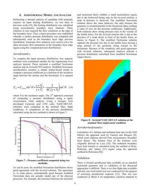
both solutions show strong pressure rises in the vicinity of
the burble fence. For the inviscid solution this is due to the
presence of a weak shock in front of the burble fence, as
shown in Figure 8. The modified Newtonian solution
captures the pressure rise due to the burble fence having a
large portion of the geometry being normal to the
freestream. Because of the simplicity and good agreement
with inviscid solutions, subsequent analyses utilized a
pressure distribution calculated from modified Newtonian
impact theory.
C P
= C P max
sin 2 ! = " + 3 #
" +1 1! 2 &
%
$ M "2 (" + 3
(
)
sin2 ! (14)
'
where θ is the incidence angle. The 2 nd approach consisted
of computing a pressure distribution using a rapid,
axisymmetric Euler analysis. Using a Georgia Tech
developed Cartesian grid CFD code, NASCART-GT,
solutions were computed at the nominal Mars flight
conditions. A comparison of the pressure distributions
calculated using the two methods is shown in Figure 7.
Pressure Coefficient, C P
2
1.8 0
!0.5 1.6
1.4 !1
1.2
!1.5
1
!2
0.8
!2.5
0.6
!3
0.4
!3.5
0.2
Mod Newtonian
Euler
!40
0 1 2 3 4 5 6
0 1 2Radial Coordinate 3 (m) 4 5 6
Figure 7 – Pressure coefficient computed using two
methods.
As can be seen, the modified Newtonian distribution shows
good agreement with the inviscid solution. The agreement
is, in some places, coincidentally good because modified
Newtonian does not actually model any of the physical
processes. For example, the transition between the aeroshell
6
Figure 8 – Inviscid NASCART-GT solution at the
nominal Mars deployment condition.
Aerothermodynamics
Calculation of a laminar and turbulent heat rate on the IAD
follows the approach used by Faurote and Burgess [9],
which used relations derived from axisymmetric boundary
layer theory. The laminar form of the relations were
originally derived by Lees [10]. The turbulent boundary
layer heat transfer is calculated using the method of Rose,
Probstein, and Adams [11] (again using the approach
outlined in Reference [9]).
Validation
There is limited aerothermal data available on an attached
isotensoid geometry and so validation of the discussed
approaches is difficult. There is no free-flight data available
and only one wind tunnel test was conducted for the purpose
of assessing aerothermal response [12]. That test was
conducted at Mach 8 on temperature sensitive material to